Propagation Effects Handbook for Satellite Systems - DESCANSO ...

1
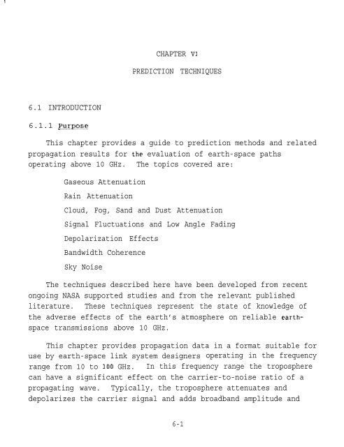
6.1 INTRODUCTION
6.1.1 purpose
CHAPTER VI
PREDICTION TECHNIQUES
This chapter provides a guide to prediction methods and related
propagation results for the evaluation of earth-space paths
operating above 10 GHz. The topics covered are:
Gaseous Attenuation
Rain Attenuation
Cloud, Fog, Sand and Dust Attenuation
Signal Fluctuations and Low Angle Fading
Depolarization Effects
Bandwidth Coherence
Sky Noise
The techniques described here have been developed from recent
ongoing NASA supported studies and from the relevant published
literature. These techniques represent the state of knowledge of
the adverse effects of the earth’s atmosphere on reliable earthspace
transmissions above 10 GHz.
This chapter provides propagation data in a format suitable for
use by earth-space link system designers operating in the frequency
range from 10 to 100 GHz. In this frequency range the troposphere
can have a significant effect on the carrier-to-noise ratio of a
propagating wave. Typically, the troposphere attenuates and
depolarizes the carrier signal and adds broadband amplitude and
6-1

phase noise to the signal. The resulting carrier-to-noise ratio
reduction reduces the allowable data rate for a given bit error rate
(digital systems) and the quality of transmission (analog systems).
In the most severe cases the medium will significantly attenuate the
carrier and destroy the transmission capabilities of the link
(termed a link outage). The frequency of occurrence and average
outage time per year are usually of most interest to system
designers. Propagation studies to date now allow the predictions to
be made with a high degree of certainty and have developed means to
reduce the frequency and length of these outages.
6.1.2 Orqanization of This Chapter
The remainder of this chapter is arranged in six relatively
independent sections covering the key topics related to the
interaction of the troposphere and earth-space propagation paths.
Each section presents a description of selected techniques and
provides sample calculations of the techniques applied to typical
communications systems parameters. A guide to the sample
calculations is given in Table 6.1-1.
6.1.3 Frequency Bands for Earth-Space Communication
—.
Within the guidelines established by the International
Telecommunication Union (ITU) for Region 2 (includes U.S. and
Canada), the Federal Communications Commission (FCC) in the U.S. and
the Department of Communications (DOC) in Canada regulate the earthspace
frequency allocations. In most cases, the FCC and DOC
regulations are more restrictive than the ITU regulations.
The services which operate via earth-space links are listed in
Table 6.1-2. The definitions of each of these services are given in
the ITU Radio Regulations. The specific frequency allocations for
these services are relatively fixed, but modifications can be
enacted at World Administrative Radio Conferences based on the
proposals of ITU member countries.
6-2

,s
Table 6.1-1. Guide to Sample Calculations
Paragraph Page
Number Description Number
6.2.4
6.2.5
6.3.2.2
6.3.2.4
6.3.3.2
6.3.5.1
6.4.3.3
6.5.6.1
6.5.6.2
6.5.6.3
6.6.2.1.1
6.6.3.3
6.6.5
6.7.3.2
6.8.3
6.8.5
6.9.2
Relative humidity to water vapor density
conversion
Gaseous Attenuation calculation
Cumulative rain attenuation distribution
using the Global Model
Cumulative rain attenuation distribution
using the CCIR Model
Cumulative rain attenuation distribution
by distribution extension
Fade duration and return period
Estimation of fog attenuation
Variance of signal amplitude fluctuations
Phase and angle-of-arrival variations
Received signal gain reduction
CCIR Approximation for rain depolarization
CCIR estimate for ice depolarization
Prediction of depolarization statistics
Group delay and phase delay
Sky noise due to clear sky and rain
Sky noise due to clouds
Uplink Noise in Satellite Antenna
6-16
6-16
6-29
6-35
6-41
6-50
6-72
6-101
6-103
6-103
6-106
6-119
6-122
6-131
6-136
6-139
6-343
A review of the Radio Regulations indicates that most of the
frequency spectrum above 10 GHz is assigned to the satellite services
or the radio astronomy service. This does not mean that the FCC or
DOC will utilize them as such, but it does highlight the potential for
use of these frequency bands. Figure 6.1-1 shows those frequency
segments not assigned for potential use by the services listed in
Table 6.1-2 (ITU-1980).
6-3

m m~ BH - ■ -m mm
1 I I 1
1 1 I 1 1 1
T 1 1 !
t
10 15 20 26 30 40 u 0030s0 90 100
FREOUENCY (Gtld
Figure 6.1-1. Frequencies Not Allocated Primarily for Earth-Space
Transmissions in Region 2
Table 6.1-2. Telecommunication Services Utilizing
Earth-Space Propagation Links
Fixed Satellite
Mobile Satellite
Aeronautical Mobile Satellite
Maritime Mobile Satellite
Land Mobile Satellite
Broadcasting Satellite
Radionavigation Satellite
Earth Exploration Satellite
Meteorological Satellite
Amateur Satellite
Standard Frequency Satellite
Space Research
Space Operations
Radio Astronomy
6-4

I
. .
6.1.4 Other Propagation Effects Not Addressed in This Chapter
6.1.4.1 Ionospheric Effects. The ionosphere generally has a small
effect on the propagation of radio waves in the 10 to 100 GHz range,
Whatever effects do exist (scintillation, absorption, variation in
the angle of arrival, delay, and depolarization) arise due to the
interaction of the radio wave with the free electrons, electron
density irregularities and the earth’s magnetic field. The density
of electrons in the ionosphere varies as a function of geomagnetic
latitude, diurnal cycle, yearly cycle, and solar cycle (among
others). Fortunately, most U.S. ground station-satellite paths pass
through the midlatitude electron density region, which is the most
homogeneous region. This yields only a small effect on propagation.
Canadian stations may be affected by the auroral region electron
densities which are normally more irregular. A more complete
discussion of the effects is included in Report 263-6 of CCIR Volume
VI 1986a) .
A mean vertical one-way attenuation for the ionosphere at 15 GHz
for the daytime is typically 0.0002 dB (Millman-1958), the amplitude
scintillations are generally not observable (Crane-1977) and the
transit time delay increase over the free space propagation time
delay is of the order of 1 nanosecond (Klobuchar-1973). Clearly for
most systems operating above 10 GHz these numbers are sufficiently
small that other system error budgets will be much larger than the
ionospheric contributions.
The one ionospheric effect which might influence wide bandwidth
systems operating above 10 GHz is phase dispersion. This topic is
discussed in Section 6.7.
6.1.4.2 Tropospheric Delays. Highly accurate satellite range,
range-rate and position-location systems will need to remove the
propagation group delay effects introduced by the troposphere.
Extremely high switching rate TDMA systems require these
corrections. The effects arise primarily due to the oxygen and
water vapor in the lower troposphere. Typical total additional
6-5

propagation delay errors have been measured to be of the order of 8
nanoseconds (Hopfield-1971).
Estimation techniques, based on the measurement of the surface
pressure, temperature and relative humidity have been developed
(Hopfield-1971r Bean and Dutton-1966, Segal and Barrington-1977)
which can readily reduce this error to less than 1 nanosecond. In
addition, algorithms for range (Marini-1972a) and range-rate
(Marini-1972b) have been prepared to reduce tropospheric
contributions to satellite tracking errors.
Since this topic is quite specialized and generally results in
an additional one-way delay of less than 10 nanoseconds it is not
addressed further in this report. An overview of this subject and
additional references are available in CCIR Report 564-3 (1986b),
and Flock, Slobin and Smith (1982).
6.2 PREDICTION OF GASEOUS ATTENUATION ON EARTH-SPACE PATHS
The mean attenuation of gases on earth-space paths in the 10 to
100 GHz frequency range has been theoretically modeled and experimentally
measured. Above 20 GHz gaseous absorption can have a significant
effect on a communication system design depending on the
specific frequency of operation. Because of the large frequency
dependence of the gaseous absorption, an earth-space communication
system designer should avoid the high absorption frequency bands.
Alternatively, designers of secure short-haul terrestrial systems
can utilize these high attenuation frequency bands to provide system
isolation.
6.2.1 Sources of Attenuation
In the frequency range from 10 to 100 GHz the water vapor
absorption band centered at 22.235 GHz and the oxygen absorption
lines extending from 53.5 to 65.2 GHz are the only significant
contributors to gaseous attenuation. The next higher frequency .
absorption bands occur at 118.8 GHz due to oxygen and 183 GHz due to
water vapor. The absorption lines are frequency broadened by
6-6

. .
collisions at normal atmospheric pressures (low elevations) and
sharpened at high altitudes. Thus the total attenuation due to
gaseous absorption is ground station altitude dependent.
6.2.2 Gaseous Attenuation
6.2.2.1 One-Way Attenuation Values Versus Frequency. The Zenith
one-way attenuation for a moderately humid atmosphere (7.5 g]m
surface water vapor density) at various ground station altitudes
(starting heights) above sea level is presented in Figure 6.2-1 and
Table 6.2-1. These curves were computed (Crane and Blood, 1979) for
temperate latitudes assuming the U.S. Standard Atmosphere, July, 45
N. latitude. The range of values indicated in Figure 6.2-1 refers
to the peaks and valleys of the fine absorption lines. The range of
values at greater starting heights (not shown) is nearly two orders
of magnitude (Leibe-1975).
Table 6.2-1. Typical One-Way Clear Air Total Zenith Attenuation
Values, A=’ (dB) (Mean Surface Conditions 21°C, 7.5 g/m3 H20; U.S.
Std. Atmos. 45°N., July)
Frequency
ALTITUDE
Okm* 0.5km l.Okm 2.Okm 4.Okm
10 GHZ ● 053 .047 .042 .033 .02
15 .084 .071 .061 .044 .023
20 .28 .23 .18 .12 .05
30 .24 .19 .16 .10 .045
40 .37 .33 .29 ● 22 .135
80 1.30 1.08 .90 .62 ● 30
90 1.25 1.01 .81 .52 .22
100 1.41 1.14 .92 .59 .25
*1 km = 3281 feet
6-7

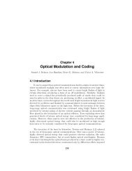
Figure 6.2-1 also shows two values for the standard deviation of
the clear air zenith attenuation as a function of frequency. The
larger value was calculated from 220 measured atmosphere profiles,
spanning all seasons and geographical locations (Crane-1976). The
smaller value applies after the mean surface temperature and
humidity have been taken into account by making the
corrections given below.
6.2.2.1.1 Dependence on Ground Station Altitude. The compensation
for ground station elevation can be done to first order by linearly
interpolating between the curves in Figure 6.2-1. The zenith oneway
attenuation for typical ground station altitudes, found in this
way? is tabulated in Table 6.2-1 for easy reference.
6.2.2.1.2 Dependence on Water Vapor Content. The water vapor
content is the most variable component of the atmosphere.
Therefore, for arid or humid regions, a correction should be made
based on the expected mean values of water vapor content.when
utilizing frequencies between 10 and 50 GHz. This correction to the
total zenith attenuation is linearly related to the mean local water
vapor density at the surface p :.
~Ac 1 = bP (PO-7.5 g/m3) (6.2-1)
where AA C1 is an additive correction to the zenith clear air
attenuation (given by Figure 6.2-1 and Table 6.2-1) that accounts
for the difference between the mean local surface water vapor
density and 7.5 g/m3. The coefficient b p is frequency dependent and
is given by Figure 6.2-2 and Table 6.2-2 (Crane ana Blood, 1979).
The accuracy of this correction factor is greatest for sea level
altitude.
“The US and Canadian weather services generally measure relative
humidity or the partial pressure of water vapor. The technique for
converting these values to p. is given in Section 6.2.5.
6-8
-.

D
1000
100
10
1
U.S. Standard Atmosphere
July, 45° N. Latitude
Mod )te Humidity
1 — Starting eights
Above St Level
.01
.001
.Ooo1
km
—
1 2 3
1
1
—
—
.
—
—
—
.
.
.
.
.
d Deviation
tier all Seasons,
TMinimum
_ Values for .
Starting
Heights of:
‘t
\
I\\,
(r
O kr 41 8,
12<
16,
/
/
f
/
‘<
~e of
ues
Sta iard Deviation v
Surl :e Temperature and]
Humidity Corrections
10 20 30 5060708090100
FREQUENCY (GHz)
I._!_
l-th
Figure 6.2-1. Total Zenith Attenuation Versus Frequency

0.001
0.0005
011003
FREQUENCY (GHz)
60 708090100
Figure 6.2-2. Water Vapor Density and Temperature
Correction Coefficients
6-10

Frequency
(GHz)
10
15
20
30
40
80
1 R
Table 6.2-2. Water Vapor Density and Temperature
Correction Coefficients
SELECT:
FREOUENCY
OROUNO STAllON AL171UOE
SURFACE WA7ER VAPOR DENSllY @ ($/ma),
OR SURFACE RELATIVE HUMID 8Y
SURFACE 7EMPERA7URE To
ELEVA710N ANOLE o
DETERMINE ZENITH AITENUATION
+’ FOR 7.S @ms U O ANO ZI°C
AT OIVEN ALT17dDE USINO
f10URES2.10RTABLE S2.1
I
COMPU7E
A~l -(bpMpo-7.5@ma)
bp OWEN IN FIOURE 6.2-2.
I
Pf) MAY BE COMPUTED FROM WEATNER
DATA - SEE SEC710N S.2-5.
I
Water Vapor Density
Correction
bP
2.1OX 10-3
6.34 X 10 -3
3.46 X 10 -2
2.37 X 10 -2
2.75x 10 -2
9*59 x 10-2
1.22 x 10-1
1 050X 10-1
,
I
I
COMPUTE
A A C 2 - CT (21% - 1~
CT OIVEN IN FIOURE 0.2.2.
I
* ?
COMPUTE
~“ . ~’+ tic, + AAc2
1
COMPUTE
AC-Ae’ CSC9
I
OETERMINE STANOARD DEVIA?lON O“ FOR
OPEAA71N0 FREOUENCY FROM FIOUFtE 8.2-1.
COMW7E
O-o” csce I
Temperature
Correction
CT
2.60 X 10 -4
4.55 x 10-4
1.55 x 10-3
1.33 x 10-3
1097 x 10-3
5.86x 10 -3
5.74 x 10-3
6.30 X 10-3
Figure 6.2-3. Technique for Computing Mean Clean Air Attenuation
6-11

6.2.2.1.3 Dependence on Surface Temperature. The mean surface
temperature TO also affects the total attenuation. This relation
(Crane and Blood, 1979) is also linear:
~Ac2 = cT (21° -TO) (6.2-2)
where TO is mean local surface temperature in ‘C.
AC2 is an additive correction to the zenith clear air attenuation.
Frequency dependent values for cT are given in Figure 6.2-2 and Table
6.2-2. As with water vapor correction, the accuracy of this factor
decreases with altitude.
6.2.2.1.4 Dependence on Elevation Anqle. For elevation angles
greater than 5 or 6 degrees, the zenith clear air attenuation AC is
multiplied by the cosecant of the elevation angle 9. The total
attenuation for arbitrary elevation angle is
A= = A=’ Csc e (6.2-3)
The standard deviation (see Figure 6.2-1) also is multiplied by the
csc 0 for arbitrary elevation angles.
6.2.3 Estimation Procedure For Gaseous Attenuation
The CCIR has developed an approximate method to calculate the
median gaseous absorption loss expected for a given value of surface
water vapor density, (CCIR-1986a). The method is applicable up to
350 GHz, except for the high oxygen absorption bands.
Input parameters required for the calculation are:
f - frequency, in GHz
0 - path elevation angle, in degrees,
h~ - height above mean sea level of the earth terminal~ in km~
and
Pw - water vapor
interest, in
density at the surface, for the location of
g/m3.
6-12

If PW is not available from local weather services?
representative median values can reobtained from CCIR Report 563-3
(CCIR-1986C).
The specific attenuation at the surface for dry air (P =
1013-mb) is then determined from:
Y. =
Y. =
7.19 x 10
[
-3 + 6.09 4.81
~+ 0.227 +
(f - 57) 2
[
3.79 x lo-’f+
for f < 57 GHz
+ 1.50
0.265 0.028
+ 1.47
(J -63)2+ 1.59 +
f2 x 10-4 dB\km
1
(f 1 x
- 118) 2
(~ + 198) 2
for 63 < f < 350 GHz
- 3
X 1 0
dB\km
[The application of the above relationships in the high oxygen
absorption bands (50-57 GHz and 63-70 GHz) may introduce errors of
up to 15%. More exact relationships are given in CCIR Report 719
(CCIR-1986d)]o
Yw =
The specific attenuation for water vapor, YW, is found from:
[
(6.2-4)
0.067 + 3 9
(f -22.3) 2
+ 7.3 +
(f - 183.3) 2
+ 6
+
4.3
10- 4 dB/km (6.2-5)
(f -323.8) 2
+ 10
1 P pw
for f < 350 GHz
The above expressions are for an assumed surface air temperature of
15”C. corrections for other temperatures will be described later.
Also, the above results are accurate for water vapor densities less
than 12 g/m3. [For higher water vapor density values, see CCIR
Report 719 (CCIR-1986d), and the followin9.1
An algorithm for the specific attenuation of water vapor which
includes a quadratic dependence on water vapor density and allows
6-13

values of water vapor densities >12 g/m3, has been proposed by
Gibbons (1986) and provisionally accepted by the CCIR (1988)~
Yw =
[ 0.050 + o.oo21p +
w
8.9
(f - 22.2) 2
‘ ( f - 325.4) 2
+ 26.3
for T = 15°C and f c 350 GHz.
3.6 10.6
1
+ 8.5 ‘(f- 183.3) 2
-I- 9.0
/2 pw 10-4 dB/km
(6.2-6)
Gibbons finds Eq. (6.2-6) to be valid within about * 15% over
the range of Pw from O to 50 g/m3. However, in applying Eq. (6.2-6)
with water vapor densities greater than 12 g/m3 it is important to
remember that the water vapor density may not exceed the saturation
value p~ at the temperature considered.
expressed as (Gibbons~ 1986)~
This saturation value may be
P. = 17.4(*) 6
where T is the temperature in ‘K.
29502
10-y
[
1
1 0
g/rn3 (6.2-7)
For temperatures in the range -20”C to +40°C Gibbons proposes a
temperature dependence of -1.0% per ‘C for dry air in the window
regions between absorption lines and -0.6% per ‘C for water vaPor.
The correction factors are therefore
Y. = YO(15 OC)[l - O.O1(TO -
15)]
(6.2-8)
Y w = YW(15 oc)[l - 0.006(T, - 15)] (6.2-9)
where To is the surface temperature in ‘C.
6-14

. .
The equivalent heights for oxygen, hO, and water vapor, hW, are
determined from:
hw =
[
2.2 +
hO=6km
hO=6+
for f < 57 GHz
40 km for 63 < Y < 350 GHz
(f - 118.7) 2
+ 1
(6.2-10)
3 1 1
(Y - 22.3) 2
km
+ 3 ‘(f- ‘(f- 1
183.3) 2
for f c 350 GHz
+ 1 323.8) 2
+ 1
(6.2-11)
The total slant path gaseous attenuation through the atmosphere, AE,
is then found.
with
For () ~ 10°:
For 6 < 10°:
A~ =
.—ho
h,
+
Y. ho e VW hw
sir 0
YO ho VW hw
AE=—
9 (ho)
+
9(%)
g(h) = 0.661% + 0.3394 ~ + 154h5.5
d
h~
4250
x = sin2El + —
where h is replaced by ho or hW as appropriate.
6-15
dB
dB
(6.2-12)
(6.2-13)
(6.2-14)
(6.2-15)

The above procedure does not account for contributions from
trace gases. These contributions are negligible except in cases of
very low water vapor densities (s1 g/m3) at frequencies
70 GHz.
above about
6.2.4 Conversion of Relative Humidity to Water Vapor Density
The surface water vapor density P. (g/m3) at a given surface
temperature TO may be found from the ideal gas law
P, = (R.H.) e~~(TO + 373) (6.2-16)
where R.H. is the relative humidity, es (N/m2) is the saturated
partial pressure of water vapor corresponding to the surface
temperature TO(OC) and RW = 461 joule/kgK = 0.461 joule/gK. A plot
of es in various units is given in Figure 6.2-4. For example, with
then
R.H. =
To = 20°c
50% = 0.5
es G 2400 n/m2 at 20°C from Figure 6.2-4
P. =
8.9 g/m3.
The relative humidity corresponding to 7.5 g/m3 at 20°C (68°F) is
R.H. = 0.42 = 42%.
6.2.5 A Sample Calculation for Gaseous Attenuation
This section presents an example calculation for the total path
gaseous attenuation, using the CCIR procedure described in Section
6.2.3.
Assume the following input parameters for a K a band link:
Frequency, Y = 29.3 GHz
Path Elevation Angle, e =
38°
6-16
-
-,

m
t
TEMPERATURE rC)
o 5 10 15 20 25 30 35
-/
CONVERSIONS
1 psia = 6895 n/m2
= 51.71 mm Hg
= 6.895 x ld dyne/cm2
= 68.95 millibsr
= 6.805 x 10 -
2 atmOs
‘c = 5/9 (°F – 32)
K = *C + 273.15
I ! I i I
30 40 50 60 70 80 90 100
TEMPERATURE (“F)
Figure 6.2-4.
6895
6000
5000
4000
.
3000:
t-
W
s
g
2000 g
3 w~
The Saturated Partial Pressure of Water Vapor Versus Temperature
1500
1000
700

Height above mean sea level, hs = .2 km
Surface water vapor density~ PW = 7.5 g/m3
Surface temperature, TO = 20°C
Step 1. Calculate the specific attenuation coefficients for oxygen,
YO, and for water vapor, YW, from Equations (6.2-4) and (6.2-6)
respectively;
Yo = 0.01763 dB/km
)’W = 0.0777 dB/km
Step 2. Correct YO and
(6.2-9) respectively;
(from fK57 GHz relationship)
YW for 20°C, using equations (6.2-8) and
?’0 = 0.01763 [1-0.01(20-15)] = 0.01675 dB/Km
Yw = 0.0777 [1-0.006(20-15)] = 0.07537 dB/Km
Step 3. Calculate the equivalent heights for oxygen, ho, and for
water vapor, hw~ from Equations (6.2-10) and (6.2-11) respectively;
ho =6km
h w = 2.258 km
Step 4. The total slant path gaseous attenuation is determined from
Equation (6.2-8);
Ag = [(0.018) (6)e-[O”zli(6J + (0.078) (2.258)1/sin (38)
= 0.1579 + 0.2764 = 004343 dB
The results show that the contribution from oxygen absorption is -
0.1579 dB, and the contribution from water vapor is 0.2764 dB, for a
total of 0.4343 dB.
6-18

6.3 PREDICTION OF CUMULATIVE STATISTICS FOR RAIN ATTENUATION
6.3.1 General Approaches
6.3.1.1 Introduction to Cumulative Statistics. Cumulative
statistics give an estimate of the total timel over a long period~
that rain attenuation or rate can be expected to exceed a given
amount. They are normally presented with parameter values (rain
rate or attenuation) along the abscissa and the total percentage of
time that the parameter value was exceeded (the “exceedance time”)
along the ordinate. The ordinate normally has a logarithmic scale
to most clearly show the exceedance times for large values of the
parameter, which are often most important. ~ Usually, the percentage
exceedance time is interpreted as a probability and the statistical
exceedance curve is taken to be a cumulative probability
distribution function. Because of the general periodicity of
meteorological phenomena, cumulative statistics covering several
full years, or like periods of several successive years, are the
most directly useful. (A technique exists, however, for extending
statistics to apply to periods greater than those actually covered.
This is described in Section 6.3.4.) Statistics covering single
years or periods would be expected to exhibit large fluctuations
from year to year, because of the great variability of the weather.
In most geographic regions, data covering ten years or more is
usually required to develop stable and reliable statistics.
Cumulative rain rate or attenuation exceedance statistics alone
give no information about the frequency and duration of the periods
of exceedance. Rather, only the total time is given. The nature of
rain attenuation, however, is such that the exceedance periods are
usually on the order of minutes in length. Different phenomena
besides rain give rise to attenuation variations occurring on a time
scale of seconds. These amplitude scintillations~ as they are
called~ are not considered in this section? but are discussed in
Section 6.5.
6-19

6.3.1.2 procedures for Calculating Cumulative Rain Attenuation
Statistics. The system designer needs reliable cumulative
attenuation statistics to realistically trade off link margins,
availability siting and other factors. Needless to say, applicable
millimeter-wave attenuation measurements spanning many years seldom
exist. It is therefore necessary to estimate statistics, using
whatever information is available.
An estimate of the rain attenuation cumulative statistics may be
determined in several ways. The optimum way depends on the amount
of rain and/or attenuation data available, and on the level of
sophistication desired. However, it is recommended that the
simplest calculations be carried out first to provide an
approximation for the statistics and also to act as a check on the
results of more sophisticated calculations.
The flow charts in Figures 6.3-1, 6.3-7 and 6.3-13 will assist
in applying selected calculation procedures. The steps are numbered
sequentially to allow easy reference with the accompanying
discussions in Sections 6.3.2, 6.3.3 and 6.3.4. These are the
procedures given:
● Analytical Estimates using the Global Model (Section 6.3.2,
Figure 6.3-l). Requires only Earth station location,
elevation angler and frequency.
. Analytical Estimates using the CCIR Model (Section 6.3.2,
Figure 6.3-7). Requires only Earth station location,
elevation angle, and frequency. -,
0 Estimates Given Rain Rate Statistics (Section 6.3.3, Figure
6.3-l). Requires cumulative rain rate exceedance statistics
for vicinity of the Earth station location, elevation angler
and frequency.
. Estimates Given Rain Rate and Attenuation Statistics (Section
6.3.4, Figure 6.3-13). Requires attenuation statistics which
6-20

LSTATION LOCATION AND ELEVATION
STEP 1
SELECT RAIN RATE
CLIMATE REGION
FROM FIGURE 6.3-2
*
STEP 2 +
SELECT SURFACE POINT
RAIN RATE DISTRIBUTION
FROM FIGURE 6.33 OR
TABLE 6.3-1
I
J
----- V
DETERMINE ISOTHERM HEIGHT H VERSUS
LATITUDE AND PERCENTAGE OF YEAR
USING FIGURE 6.3.4
DEVELOP AN ISOTHERM HEIGHT H VERSUS
PERCENTAGE PLOT
COMPUTE HORIZONTAL PROJECTION
(BASAL) LENGTH OF PATH IN KM
I
H–H. IF O > 22.5km, ADJUST L
D =~ PROB. OF OCCURRENCE = SELECTED
tan O
PROBABILITY {0/22.5)
STEP 6 4
COMPUTE EMPIRICAL CONSTANTS
FOR EACH PERCENTAGE VALUE:
X = 2.3 RP-Q”’7
Y = 0.026-0.03 In Rp
Z = 3.8 – 0.6 In RP
U=}ln[XeYzli /2
STEP 7 1
COMPUTE TOTAL ATTENUATION, A (dB) :
a)l FO>Z
KRpa JJzof, ~beYZCY + ~beY
A=——-——
CC6 e [ Ub Yb Yb7
b)lF D

may be for frequency and elevation angle different from those
needed.
6.3.1.3 Other Considerations. Generally the yearly cumulative
statistics are desired. The worst-month or 30-day statistics are
sometimes also needed, but are not derivable from the data presented
here. Worst 30-day statistics are discussed in Section 6.3.7.
The attenuation events due to liquid rain only are considered
here. Liquid rain is the dominate attenuation-producing
precipitation because its specific attenuation is considerably
higher than snow, ice, fog, etc. The contribution of these other
hydrometers is estimated in later sections.
The cumulative statistics are appropriate for earth-space paths
for geostationary or near-geostationary satellites with relatively
stable orbital positions. The modifications required to develop
statistics for low-orbiting satellites is unclear because of the
possibly nonuniform spatial distribution of rain events arising from
local topography (lakes, mountains, etc.). However, if one assumes
these effects are of second-order, low orbiting satellites may
simply be considered to have time-dependent elevation angles.
6.3.2 Analytic Estimates of Rain Attenuation from Location and Link
Parameters
The following analytic estimation techniques provide reasonably
precise estimates of rain attenuation statistics. The first
technique is based on the modified Global Prediction Model (Crane
and Blood- 1979, Crane- 1980, 1980a). Only parts of the model
relevant to the contiguous US and Canada, and elevation angles
greater than 10°, are presented here. The second technique uses the
CCIR Model and is perhaps the simplest prediction approach. Example
applications of both techniques are given. The analytical
developments for the global model and the CCIR model are presented
in Sections 3.4 and 3.6? respectively.
6-22
-

The models require the following inputs:
a) Ground station latitude, longitude and height above mean sea
level
b) The earth-space path elevation angle
c) The operating frequency
6.3.2.1 ~c>bal Model Rain Attenuation Prediction Technique.
6.3-1 gives the step-by-step procedure for applying the Global
Figure
Model. The steps are described in detail below.
Step 1 - At the Earth terminal’s geographic latitude and
longitude, obtain the appropriate climate region using Figure
6.3-2. For locations outside the Continental U.S. and Canada,
see Section 3.4.1. If long term rain rate statistics are
available for the location of the ground terminal~ they should
be used instead of the model distribution functions and the
procedure of Section 6.3.3 should be employed.
Step 2 - Select probabilities of exceedance (P) covering the
range of interest (e.g.~ .OIJ .1 or 1%). Obtain the terminal
point rain rate R (mm/hour) corresponding to the selected values
of P using Figure 6.3.3, Table 6.3-1 or long term measured
values if available.
Step 3 - For an Earth-to-space link through the entire
atmosphere, obtain the rain layer height from the height of the
0° isotherm (melting layer) Ho at the path latitude (Figure 6.3-
4). The heights will vary correspondingly with the
probabilities of exceedance, P. To interpolate for values of P
not given, plot HO (P) vs Log P and sketch a best-fit curve.
Step 4 - Obtain the horizontal path projection D of the oblique
path through the rain volume:
HO-H 9;9210°
D=—
tanO
6-23
(6.3-1)

m
I
NJ
Q
Figure 6.3-2. Rain Rate Climate Regions for the Continental U.S. and Southern Canada

I
z za
E 100
g
w
~
z
z K 50
a) ALL REGIONS
n
6.001 0.01 0.l
1,0 10.0
PERCENT OF YEAR RAIN RATE VALUE EXCEEDED
b) SUBREGIONS OF THE USA
1 1 1 I I 1 1 I 1 I I 1 1 11 I 1 I I , I 111 # I I 1 1 1 11
0
0.001 0.01 0.1 1,0 10,0
PERCENT OF YEAR RAIN RATE EXCEEDED
Figure 6.3-3. Point Rain Rate Distributions as a Function of
Percent of Year Exceeded

Table 6.3-1. Point Rain Rate Distribution Values (mm/hr) Versus Percent of Year
Rain Rate is Exceeded
Percent
of Year
0.001
0.002
0.005
0.01
0.02
0.05
0.1
0.2
0.5
1.0
2.0
5.0
A
28.5
21
13.5
10.0
7.0
4.0
2.5
1.5
0.7
0.4
0.1
0.0
‘1
45
34
22
15.5
11.0
6.4
4.2
2.8
1.5
1.0
0.5
0.2
B
57.5
44
28.5
19.5
13.5
8.0
5.2
3.4
1.9
1.3
0.7
0.3
‘2
70
54
35
23.5
16
9.5
6.1
4.0
2.3
1.5
0.8
0.3
c
78
62
41
28
18
11
7.2
4.8
2.7
1.8
1.1
3.5
RAIN CLIMATE REGION
‘1
90
72
50
35.5
24
14.5
9.8
6.4
3.6
2.2
1.2
0.0
D= D 2
108
89
64.5
49
35
22
14.5
9.5
5.2
3.0
1.5
0.0
‘3
126
106
80.5
63
48
32
22
14.5
7.8
4.7
1.9
0.0
E
165
144
118
98
78
52
35
21
10.6
6.0
2.9
0.5
F
66
51
34
23
15
8.3
5.2
3.1
1.4
0.7
0.2
0.0
G
185
157
,20.5
94
72
47
32
21.8
12.2
8.0
5.0
1.8
253
220.5
178
147
119
86.5
64
43.5
22.5
12.0
5.2
1.2
~intJtes Hours
per per
Yea r Year
5.26 0.09
10.5 0.18
26.3 0.44
52.6 0.88
105 1.75
263 4.38
526 8.77
1052 17.5
2630 43.8
5260 87.7
10520 175
26298 438
. .

B
.
. .
t-
I I I I I 1
11/1
-
. .
. -----
6-27
0
m m
z
.C-4
$

HO = HO(P) = height (km) of isotherm for probability P
Hg = height of ground terminal (km)
6= path elevation angle
Test D S 22.5 km; if true, proceed to the next step. If D 2 22.5
km, the path is assumed to have the same attenuation value as for a
22.5 km path but the probability of exceedance is adjusted by the
ratio of 22.5 km to the’ path length:
New probability of exceedance, P’ = P (W”)
(6.3-2)
where D = path length projected on surface. This correction
accounts for the effects of traversing multiple rain cells at low
elevation angles.
Step 5 - Obtain the specific attenuation coefficients, k and a?
at the frequency and polarization angle of interestr from Table
6.3-3. For frequencies not in the table, use logarithmic
interpolation for K and linear interpolation for a. The
subscript H columns are for horizontal linear polarization and
the subscript V columns are for vertical linear polarization.
[For polarization tilt angles other than horizontal or vertical,
use the relationships on Figure 6.3-6~ Step 4, to obtain K and
a].
Step 6 - Using the RP values corresponding to each exceedance
probability of interest~ calculate the empirical constants X, Y,
Z and U using
x= 2.3 RP ‘0”17
Y = 0.026 - 0.03 in R p
z = 3.8 - 0.7 in R p
u= [ln(XeYz)]/z”
6’-”28
(6.3-4)
(6.3-5)
(6.3-6)
(6.3-7)

.-
.
9
s@EQ - If Z S D, compute the total attenuation due to rain
exceeded for P % of the time using
A=
kRp@ #Z~.1
—-
Cose UQ
[
where A= Total path attenuation
k, a = parameters relating
(from Step 5).
RP = point rain rate
e = elevation angle of path
)(cYeWcY
ya
+
~YDa
due to rain (dB)
yu ;6;10”
(6.3-8)
1
the specific attenuation to rain rate
D = horizontal path projection length (from step 4)
If D< Z,
If D = 0,0 = 90°,
~a em-l
A=
Cos e [1 Ua
(6.3-9)
A=” (H - Hg)(K RPa) (6.3-10)
This procedure results in an analytical estimate for the
attenuation, A, exceeded for P percent of an average year. The use
of a programmable calculator or computer for performing these
calculations is highly recommended.
6.3.2.2” A Sample Calculation for the Global Model. The following
information is given for the Rosman~ NC Earth Station operating with
the ATS-6 satellite.
Earth station latitude :.
Earth station longitude:
Earth station elevation:
6-29
35°N
277°E.
0.9 km

Antenna elevation Angle: 47°
Operating frequency: 20 GHz
We wish to find an analytic estimate for the cumulative attenuation
statistics using the procedure of Figure 6.3-1.
1. Select rain rate climate region for Rosman, NC:
From Figure 6.3-2, Rosman is located in region D3.
2* Select surface point rain rate distribution:
From Table 6.3-1, region D3 has the following distribution:
% RP
— —
0.01 63
0.02 48
0.05 32
0.10 22
0.20 14.5
0.50 7.8
1.0 4.7
3. Determine isotherm height H:
From Figure 6.3-4, the following isotherm height estimates apply
at 35° latitude.
0.01 4.4 km
0.1 3.75
1.0 3.2
By plotting these, the following additional points may be
interpolated
6-30

1
0.02
0.05
0.2
0.5
4. Compute D:
Using e = 47° and H g
0.01
0.02
0.05
0.1
0.2
0.5
1.0
5. Select K and a:
4.2
3.95
3.55
303
= 0.9 km, we obtain
3.25 km
3.1
2.85
2.65
2.45
2.25
2.15
The specific attenuation coefficients, K and a are selected
from Table 6.3-3 at 20 GHz, horizontal polarization.
K= 0.0751
a = 1.10
6. Compute empirical constants:
For E?xamplet
~ ~ g g g
0.1 1.36 -0.067 1.95 0.091
0.2 1.46 -00054 2.20 0.118
6-31

0.5 1.62 -0.036 2.57 0.153
7. Compute attenuation, A:
We note from step 6 that at 0.2%, D is greater than Z= This
also holds for percentages less than 0.1%. Thus the formula of
Step 7 (a) is used to find the attenuation for % S 0.1.
For % 2 0.5, D is less than Z, so the formula of Step 7 (b)
applies. The attenuation values found in this way are plotted
versus percentage exceedance in Figure 6.3-5. The figure
includes statistics derived from 20 GHz attenuation measurements
made at Rosman with the ATS-6 over a 6-month period.
6.3.2.3 CCIR Model Rain Attenuation Prediction Technique
This section presents the step by step procedure for application
of the CCIR rain attenuation prediction model, described in detail
in Section 3.6. The procedure is outlined in Figure 6.3-6.
Step 1 Obtain the rain rate, ROaOl, exceeded for 0.01% of an average
year for the ground terminal location of interest. If this
information is not available from local data sources, an estimate
can be obtained by selecting the climate zone of the ground terminal
location from Figure 6.3-7, and the corresponding rain rate value
for that climate zone from Table 6.3-2. (For locations not found on
Figure 6.3-7, see Figures 3.6-1 and 3.6-2).
[Important Note: The CCIR rain climate zones are ~ the same as
the climate regions of the Global Model described earlier. ]
6-32

I
.
,.
.
~
q
8
H
v
~
1.0
0.8
0.6
0.4
0.2
z
o
i=
a
g 0.1
t-
: 0.08
a
$’
~ 0.06
#
0.04
0.02
0.01
.
.
.
.
.
.
.
.
.
.
.
.
.
-
—
O ATS-6 DATA, OBTAINED
FROM 6-MO. STATISTICS
BY DISTRIBUTION
EXTENSION TECHNIQUE
{Seo Pare. 6.3.4.2)
A ANALYTIC ESTIMATE
1 1
6 10 15 20 25 30 35
ATTENUATION AT 20GHz (dB)
Figure 6.3-5. Analytic Attenuation
Actual Measurements
6-33
Estimate and

Table 6.3-2. Rain Rates Exceeded for 0.01% of the Time
Climate ABCDEFG HJKLMNP
Rate 8 12 15 19 22 28 30 32 35 42 60 63 95 145
SteR 2 Determine the effective rain height, hr, from;
hr = 4.0
= 4.0 - 0.075 (
+- 361 +: j6~< 36°
(6.3-11)
where $is the latitude of the ground station, in degrees N or S.
W Calculate the slant path length? h~ horizontal Projection
LG, and reduction factor, rpr from:
For @ ~ 5°,
= (h r - hO)/sin (@) (6.3-12)
LG = L~ COS (@) (6.3-13)
rp (6.3-14)
1 + 0.~45LG
where @ is the elevation angle to the satellite~ in degrees~ and ho
is the height above mean sea level of the ground terminal location~
in km. (For elevation angles less then 5°~ see Section 306).
Step 4 Obtain the specific attenuation coefficients~ K anda, at the
frequency and polarization angle of interest from Table 6.3-3. For
frequencies not on the table, use logarithmic interpolation for K
and linear interpolation for a. For polarization tilt angles other
than linear horizontal or vertical, use the relationships on Figure
6.3-6, Step 4, to obtain K and a.
Step 5 Calculate the attenuation exceeded lar 0.01% of an average
year from;
Ao,o1 = K Ro.01~ LS r p (6.3-15)
6-34

Step 6 Calculate the attenuation exceeded for other percentage
values of an average year from:
AP = 0012 AOCO1 p-(0.546 + 0.043 109 P] (6.3-16)
This relationship is valid for annual percentages from 0.001% to
1.0%.
6.3.2.4 Sample Calculation for the CCIR Model
In this section the CCIR model is applied to a specific ground
terminal case. Consider a terminal located at Greenbelt, MD., at a
latitude of 38°N, and elevation above sea level of 0.2 km. The
characteristics of the link are as follows:
Frequency: 11.7 GHz .
Elevation Angle: 29°
Polarization: Circular
Step 1 Figure 6.3-7 indicates that the terminal is in climate zone
K, with a corresponding RO,Ol f 42 mm/h (Table 6.3-2).
Step 2 The effective rain height, from Eq (6.3-11), is
hr = 4.0 - 0.075(38 - 36) = 3.85
Step 3 ‘I’he slant path length, horizontal projection, and reduction
factor are determined from Eq.’s (6.3-12, -13, -14) r@spectiv@ly:
Ls = (3.85 - 0.2)(/sin(29°) = 7.53
LG = (7.53)cos(29°) = 6.58
rp = 1/[1 + (0.045)(6.58)] =
o.771
6-35

Step 4 The specific attenuation coefficients are determined by
interpolation from Table 6.3-3, with a polarizaiton tilt angle of
45° (circular polarization);
Step 5 The
Eq. (6.3-15
K= o.o163, a = 1.2175
attenuation exceeded for 0.01% of an average year, from
~ is;
Ao.ol = (0.0163) (42)1.217S(7.53) (0.771 )
= 8.96 dB
Step 6 The attenuation exceeded for other percentages is then
determined from Eq. (3.6-16);
% Attenuation (dB)
1.0 1.08
0.5 1.56
0.3 2.02
001 3(42
0.05 4.67
0.03 5.80
0.01 8.96
0.005 11.48
0.003 13.65
0.001
19.16
Figure 6.3-8 shows a plot of the resulting attenuation prediction
distribution, compared with three years of measured distributions
obtained with the CTS satellite (Ippolito 1979). The CCIR
prediction is seen to over-predict slightly for higher percentage
values, and to vastly under-predict for percentages below about
0.01%0
6-36

m I
:
STEP 1
SELECT CLIMATE ZONE
FROM FIGURE 6.3-7
AND RAIN RATE ROW
FROM TABLE 6.3-2
I
STEP 2 +
DETERMINE THE EFFECTIVE
RAIN HEIGHT IN KM FROM
THE LATITUDE O IN DEGREES
~ = 4.0 FOR050
~
K = [~ + K v + (~ - KvkM? 0 cos 211/2
K#?H + K V U V + (~a” - KvUvlcas28 COS 2T
T = POLARIZATION TILT ANGLE RELATIVE
TO HORIZONTAL (t = 46° FOR
CIRCULAR POLARIZATIONI
STEP 5
CALCULATE ATfENUATION EXCEEDED
FOR 0.01 % OF TIME
AWN
= L, rp KRa
t
I
.
STEP 6 +
CALCULATE AITENUATION EXCEEDED
FOR P% OF TIME
Ap =0.12A ‘(0.546+ 0.043 log P)
0.01 p
FOR O.W1 % < p < 1.0°4
Fiaure 6.3-6. Analytical Estimate Procedure for Cumulative Rain Rate and
.
Atte~uation Statistics Using the CCIR Model

16s 0
30°
0°
30°
[
t
A
. . .
13s0 105° 75” 45”
D
A
~’—” “-
““ 165° 135° 1o5- #a
E
Q
c
v
a— F
—
ls O
E 4!H
45°
30°
++00
A
/
— 30°
Figure 6.3-7. CCIR Rain Climate Zones for ITU Region 2
6-38
60°
15°

9
10.OOOO
1.0000
0,1ooo
0.0100
0.0010
I=’ ’’’l ’’’’ l’’’ ’’l ’’’’ l’ ’’’l’” ‘1’’”
F
11.7GHZ.
GREENBELT, MD.
L
“\
\
\
\ \
.
[[
\\.
\\
\ \“\\\“\
MEASUREMENTS
FIRST YEAR
---- SECOND YEAR
● - - - - - THIRD YEAR
CCIR PREDICTION
I \“\
\

Frequency
(Gtiz)
1
2
4
6
8
10
12
15
20
25
30
35
40
45
50
60
70
80
90
100
120
150
200
300
400
Table 6.3-3. Regression Coefficients for Estimating
Specific Attenuation in Step 4 of Figure 6.3-6
‘H
0.0000387
0.000154
0.000650
0.00175
0.00454
000101
0.0188
0.0367
0.0751
0.124
0.187
0.263
0.350
0.442
0.536
0.707
0.851
0.975
1.06
1*12
1.18
1.31
1.45
1.36
1,32
‘v
0.0000352
0.000138
0.000591
0.00155
0.00395
0.00887
0.0168
0.0347
0.0691
0.113
0.167
0.233
0.310
0.393
0.479
0.642
0.784
0.906
0.999
1.06
1.13
1.27
1.42
1.35
1.31
aH
0.912
0.963
1.12
1.31
1.33
1.28
1.22
1.15
1.10
1.06
1.02
0.979
0.939
0.903
9.873
0.826
0.793
0.769
0.753
0.743
0.731
0.710
0.689
0.688
0.683
av
o ● 880
0.923
1.07
1.27
1.31
1,26
1.20
1.13
1.07
1.03
1.00
0.963
0.929
0.897
0.868
0.824
0.793
0.769
0,754
0.744
0,732
0.711
0.690
0.689
0.684
* Values for k and a at other frequencies can be obtained by interpolation
using a Iogarlthmjc scale for k and frequency and a linear scale for a
6-40

1
6.3.3 Estimates of Attenuation Given Rain Rate Statistics
6.3.3.1 Discussion and Procedures. If the rainfall statistics can
be reconstructed from Weather Service data or actual site
measurements exist for a period of at least 10 years near the ground
station site~ these may be utilized to provide’ Rp versus percentage
exceedance. The temporal resolution required of these measurements
is dependent on the smallest percentage resolution required. For
example, if 0.001% of a year (5.3 minutes) statistics are desired,
it is recommended that the rain rate be resolved to increments of no
more than l-minute to provide sufficient accuracy. This can be done
utilizing techniques described in Chapter 2 of this handbook, but 5minute
data is more easily obtained.
The cumulative statistics measured near the ground station site
replaces Steps 1 and 2 of Figure 6.3-1. The attenuation statistics
are generated using the procedures in Steps 3 through 7 of Figure
6.3-1.
6.3.3.2 Example. Again we take the case of the 20 GHz ATS-6 link
to Rosman, NC. We have cumulative rain rate statistics for Rosman
for a six-month period as shown in Figure 6.3-9. (Data spanning
such a short period should not be used to estimate long-term
statistics. The use here is for demonstration purposes only.) We
first select values of rain rate R corresponding to several values
of percentage exceedance. :
%
—
0.01
0.02
0.05
0.10
0.20
0.50
1.0
R p
—
66
55
34
16.5
10.5
4.5
2.3
6-41

~
o
1.0 1
0.90
0.80
0.70
0.60
0.60
0.40
0.30
8 a8 o.2a
Lu wu~
z oi= ● o
b ● o
w
~ .0
z
Lu
$ .0
w
&
.a
.(
J
.
.
.
.
.
10 20
POINT RAIN RATE (mm/hr)
30 40 50 60 70
I 1 1 I I I
20 GHz, ATS.6, ROSMAN, NC
O RAIN RATE DATA (6 MONTHS)
/J ATTENUATION ESTIMATE FROM
RAIN RATE STATISTICS
o
ATS-6 ATTENUATION DATA FROM
DISTRIBUTION EXTENSION TECHNIQUE
[See Para. 6.3.4.2)
~30
10 16 20
35
0
6
ATTENUATION (dB) AT 20 GHz
Figure 6.3-9. :tenuation Statistics Estimate Based on Measu”red
Rainfall Statistics
6-42
#

●
We now proceed exactly as in the Global Model application
example (Section 6.3.2.2)~ using these values of R p instead of those
in Table 6.3-1 or Figure 6.3-3.
The results of these calculations are shown in Figure 6.3-9,
along with the measured attenuation statistics. This data is
presented to demonstrate the technique. More accurate data,
covering a longer periodl is presented in Chapter 5.
6.3.4 Attenuation Estimates Given Limited Rain Rate and Attenuation
Statistics
6.3.4.1 Discussion and Procedures. The system designer will
virtually never find attenuation statistics spanning a number of
years for his desired location, operating frequency and elevation
angle. But by applying distribution extension and scaling
procedures to the limited statistics available, the designer my
make useful estimates of the statistics for the situation at hand.
Distribution extension allows one to take concurrent rain rate
and attenuation measurements intermittently over a limited period of
time, then convert the data into cumulative attenuation statistics
covering the entire year. The conversion requires stable cumulative
rain rate statistics for the site or a nearby weather station~ and
measurements taken over a statistically significant fraction of the
year. Distribution extension is required in practice because it is
often costly to make continuous attenuation measurements over
extended periods. Rather, data are taken only during rainy periods.
Scaling is required to account for differences between the
frequency and elevation angle applying to the available statistics,
and those applying to the actual system under consideration. This
scaling is based on empirical formulas which~ to the first order
approximation depend only on the frequencies or the elevation angle
and apply equally to all attenuation values. To a better
approximation, however, the rain rate corresponding to the
attenuation and other factors must be considered as well.
6-43

Figure 6.3-10 shows a generalized procedure for applying the
distribution extension and scaling techniques described in this
section.
6.3.4.2 Attenuation Distribution Extension. The technique is
illustrated in Figure 6.3-11. The upper two curves represent
cumulative rain rate and attenuation statistics derived from
measurements taken over some limited period of time. The
measurement time may consist for example, of only the rainy periods
from April through September. The exceedence curves are plotted as
functions of the percentage of the total measurement time. The
lower solid curve represents the cumulative rain rate statistics,
measured over an extended period at the same location as the
attenuation measurements, or derived from multi-year rainfall
records from a nearby weather station.
A curve approximating the long-term cumulative attenuation
distribution (the bottom curve in Figure 6.3-11) is derived from the
three upper curves by the following graphical procedure:
10 Select a percent exceedance value, El, and draw a horizontal
line at that value intersecting the limited-time rain rate
and attenuation distribution curves at points a and b~
respectively.
2. At the rain rate value R corresponding to El, project a line
down to intersect (at point c) the long-term rain rate curve
at the exceedance value E2.
3. At the attenuation value A corresponding to El, project a
line down to the exceedance value Ez. This (point d) is a
point on the long-term attenuation curve.
6-44

STEP 1
GIVEN:
STATION PARAMETERS
SATELLITE PARAMETERS
OPERATING FREQUENCY, fw
LIMITED RAIN STATI!5WS
LIMITED ATTENUATION
STATISTICS AT fmea
COMPUTE: CUMULATIVE ATTENUATION
STATISTICS, DISTRIBUTION EXTENSION
STEP 2A
‘w= ‘rne~
6W=*
COMPUTE:
CUMULATIVE
ATTENUATION
STATISTICS
fop # fme~
eOP + e
STEP 3
STEP 4
STEP 5
STEP 20
FREQUENCY SCALE ELEVATfON
ATTENUATIONS ew+o SCALE AITENUATION
READINGS ‘ READING
Figure 6.3-10. procedure for Generation of Cumulative Attenuation
Limited Rain Rate and Attenuation Statistics
Statistics Given
1

El
E2
.
.
.
.
.
.
.
.
.
.
1
\
.
----.---—
-.—-
\
\
\
\
I
I
\
LIMITED-TIME
ATTENUATION STATISTICS
LONG-TERM
I AITENUATION DISTRIBUTION
i I
I
I
I
I
R!
) 1 I 1 1 1 1 1 1 1 1 1 1
RAIN RATE
J
[ 1 1 1 II 1 1 1 1 1 1 1 1
RAIN ATTENUATION
Figure 6.3-11. Construction of Cumulative Attenuation Statistics
Using the Distribution Extension Technique
6-46

.
B
.
. .
4. Repeat the process for several points and join them with a
smooth curve.
Distribution extension in this manner assumes that the values
rain rate and attenuation renain the same as the measured values~
the average, for times of the year different than the measurement
period. This is not necessarily so. The physical distribution of
raindrops along the propagation path in a stratiform rain, for
example, differs from the distribution in a mild convective storm.
Both conditions could produce local rainfall at the same rate, but
the attenuation produced could be quite different. Thus in regions
where there is wide seasonal variation in how rain falls~
distribution extension should be used with caution. The reliability
of the extended distribution depends on how “typical” of the whole
year the rainfall was during the measurement period. If the shapes
of the limited-time and the long-term distribution curves are
similar, the limited-time sample is statistically significant and
the distribution extension will be valid.
6.3.4.3 Frequency Scalinq. If frequency scaling of measured rain
attenuation (Step 3 of Figure 6.3-10) is required~ the specific
attenuation scaling technique is recommended. In this technique
specific attenuation data is utilized to scale the attenuation A
from frequency fl to frequency fz. Referring to the equation for rain
attenuation in Step 7 of Figure 6.3-1, the result is
where
of
on
(6.3-17)
A, = A1(fl)~ Az = A2(f2), kl = kl(fl), . . . , etc. (6.3-18)
This is a fair estimate for small frequency ratios (e.g.r less than
1.5:1), and moderate rain rates~ but errors can be large otherwise.
This is because the above equation implicity assumes that rainfall
6-47

is homogeneous over the propagation path, which is usually not true.
By assuming a simple Gaussian model for the rain rate with distance
along the pathr Hedge (1977) derived an expression for attenuation
ratio that includes an inhomogeneity correction factor, and uses the
high correlation between attenuation and peak rain rate to eliminate
the rain rate:
This yields a better fit to empirical data.
(6.3-19)
6.3.4.4 Elevation Anqle Scalinq. Step 5, the elevation angle
scaling between the operational elevation angle OOP and the measured
data angle omea~ is somewhat complex. The first order approximation,
the cosecant rule, is recommended, namely
A(e~) = Csc e2 = sin el
A(e]) csc e, sin 02
If more detailed calculations are desired the full formulas in
Figure 6.3-1 are utilized.
(6.3-20)
6.3.4.5 Example of Distribution Extension. Figure 6.3-12 shows an
example of applying the distribution extension technique. The upper
two curves are cumulative rain-rate and attenuation statistics
derived from more than 600 total minutes of measurements over the
July through December 1974 period. The bottom curve in the figure
is the measured distribution of rain rate for the entire six-month
period (263,000 minutes). Comparison of the two rain rate
distributions shows that they are very similar in shape. This
indicates that the rain rate measurements made during attenuation
measurements are a statistically significant sample of the total
rainfall, and that using the distribution extension technique is
6-48

. .
●
100
10
1.0
.1
.01
.
.
RAIN RATE (mm/hr)
10 20 30 40 50 w 70
MEASURED ATTENUATION
~ 608 MINUTES TOTAL
\
Figure 6.3-12.
PREDICTED
. ATTENUATION
BY DISTRIBUTION \
. EXTENSION
< ~ TECHNIOUE
(
.
20 GHz ATTEN. PREDICTION
JULY THRU DEC/74
MINUTELY AVERAGES
ROSMAN, N.C.
RAIN RATE DURING
MEASUREMENTS
\
MEASURED RAIN RATE
OVER 6 MONTH PERIOD
ATTENUATION
1 I I I 1
6 10 15 20 25 30 35
ATTENUATION (dB)
Example of Distribution Extension Technique
6-49

valid. The extended attenuation distribution, constructed as
described in paragraph 6.3.4.2, is shown in the figure.
6.3.5 Fadinq Duration
System designers recognize that at some level of rain rate Rm
the entire system margin will be utilized. The cumulative rain rate
statistics indicate the percentage of time the rain rate exceeds R m.
In this section, a technique is presented for estimating an upper
bound on the duration of the periods that the rain rate exceeds a
given Rm. This is equivalent to the duration of fades exceeding the
depth corresponding to R m.
Experimental fade duration statistics are presented in Chapter 5
(Section 5.6). As mentioned in that section, experimental data has
confirmed that the duration of a fade greater than a given threshold
tends to have a log-normal probability distribution. This is
equivalent to the logarithm of the duration having a normal
distribution. Given sufficient experimental data, one ma-y determine
the parameters of the best-fitting log-normal distribution, and use
these to extrapolate from the empirical distribution. Such
extrapolation could be used in lieu oft or in addition to~ the
technique described here when fade duration data is available.
6.3.5.1 Estimating Fade Duration Versus Frequency of Occurrence.
The US and Canadian weather services have published maximum rainfall
intensity (rain rate) - duration - frequency curves which provide
the point rain rates for several hundred locations on the North
American continent (U.S\ Dept. Comm.-l955 and Canada Atmos. Env.-
1973) ● Two typical sets of curves for the close-proximity cities of
Baltimore, MD and Washington, D.C. are shown in Figure 6.3-13. The
return periods are computed using the analysis of Gumbel (1958)
since data is not always available for the 100-year return period.
These curves are derived from the single maximum rain-rate event in
a given year and are termed the annual series. For microwave
propagation studies, curves that consider all high rain rate events
are necessary. Such curves, called the partial-duration series~ are
6-50
-

not normally available~ but empirical multipliers have been found
for adjusting the annual series curves to approximate the partialduration
series (Dept. COmmerce-1955). TO Obtain the partialduration
curve, the rain rates on the annual series curve for the
desired return period are multiplied by the appropriate factors,
given in Table 6.3-4.
Table 6.3-4. Multiplicative Factors to Convert Annual
to Partial-Duration Series
RETURN PERIOD (YEARS)
MULTIPLY ANNUAL SERIES
RAIN RATE BY
2 1.13
5 1.04
10 1.01
25, 50, 100 1.00
6-51

20.0
15.0
!$ 10.0
x 8.0
E 6.0
n.
E
II I
I Ill I I I 1 I 1 II I 1
I I I I
~ NOTE ~
_ FREQUENCY ANALYSIS BY METHOD OF
~XTR~ME VA\UES, A~ER f3UMB~L 4
I l l II I a
I Ill I 1 Ill Ill 1 1
0.1 -.. .
5 10 1520 30405060 2 3456 61012 1824
20.0
15.0
a
> 10.0
~ 8.o
f 6.0
u
8
~ 2,0 .
; ,.0
Z 0.8
# 0.6
$
$ 0.2
K
MINUTES HOURS
DURATION
FREQUENCY ANALYSIS BY MEfHOO OF
EXTREME VALUES, AFTER WMSEL
0.1 1111 I 1 1 1 1 1 I l.+
5 10 20 4 0 8 0 2 4 8 10 24
MINUTES HOURS
DURATION
WASHINGTON, D.C.
1696-1897, 1899-1953
BALTIMORE, MARYLAND
1903-1951
Figure 6.3-13. Typical Rain Rate-Duration-Frequency Curves.
From U. ‘.. Weather Service, Annual Series
6-52

●
The intensity-duration-frequency curves actually give the
average rain rate over the duration period, whereas the
instantaneous rain rate is of interest from a propagation
standpoint. The curves therefore do not directly give the frequency
ver-sus duration of fades of a given depth. However, for short
averaging periods (e.g., five minutes), the instantaneous rain rate
would be expected to stay fairly close to the average rain rate, and
would certainly never exceed it for the entire period. The curves
then can be used to approximate the frequency of short-duration
fades, and to place an upper bound on the frequency in any case.
The minimum return period shown on Figure 6.3-13 is two years.
It is desirable to be able to extrapolate to one year. This can be
done using the Gumbel frequency analysis technique for extreme
values. This has been accomplished graphically, for durations of 5
through 60 minutes as shown in Figure 6.3-14. The data used in the
curves has been adjusted using the multipliers of Table 6.3-4 to
correspond to the partial-duration series. For example, the rain
rate expected in Baltimore in a 5-minute period once in 2 years is
5.2 X 1.13 = 5.9 inches per hour, Extrapolating to one year yields
4.8 inches per hour (122 mm/h). Similar calculations may be done
for other duration periods to generate a l-year return period curve
for the partial-duration series.
The recommended technique for estimating the maximum fade period
to be expected in an N-year rain event is described in Figure
6.3-15. Here the station parameters (latitude, longitude, etc.),
operating frequency and link margin (after clear air attenuation is
removed) are required inputs. By iteratively solving the
attenuation equation in Figure 6.3-1 the maximum allowable point
rain rate RPm is obtained. The estimate of the maximum fade duration
for the worst rain in 1,2,5,10 or more years is then obtained from
data for the partial-duration series rain rate-duration-frequency
curves (see Figure 6.3-9). For example, if the system maximum
allowable rain rate RPm is 5 inches/hour (125 mm/hr), a system in
6-53

100 -_
50
5-MINUTE RAIN RATE
?-
1 I I 1 I .
&- -d OTTAWA
~ BALTIMORE
~
S -. +3 WASHINGTON, D.C. 4
@
+20
,
I
0
s 10
K
UJ
a
!5 -
a
2
{
/
/
P .
/ /
// /:
1/ /
& I 1 I 1
0 2 4 6 8 10 12
50 .
!f
s ● 2O
I
o ~
s 10
a
u
n
a
RAIN RATE – INCHE.SIHOUR
lSMINUTE RAIN RATES
-“Q WASHINGTON, D.C.
2
r
I
1 1 1 I 1 1 1
0 2 4 6 8 10 12
RAIN RATE - INCHESIHOUR
1O-MINUTE RAIN RATE
100 ~ 1 I 1 1
50
.
~
s
*2O
P
I
o
: 10 .
1’ . //
#
!5 -
a
2
100
so I
)
●
* 9
/
/“
.
& -
4 OTTAWA
~ BALTIMORE
q WASHINGTON, DC.
/ {~
1 1 I I
o 2 4 6 8 10 12
2
RAIN RATE - INCHESIHOUR
30-MINUTE RAIN RATES
1
r
.
C+.a WASHINGTON, D.C.
I I I 1
0 1 2 3 4 5 6
RAIN RATE - INCHESIHOUR
Figure 6.3-14. Extrapolated Partial-Duration Rain
Rate-Duration-Frequency Curves
6-54

-
GIVEN:
STATION PARAMETERS
OPERATING FREQUENCY,
LINK RAIN MARGIN, M(dB)
I
STEP 1
ESTIMATE MAXIMUM POINT RAIN RATE Rpm
BY ITERATIVELY SOLVING
ATTENUATION EQUATION IN
FIGURE 6.3.1 WITH ATTENUATION = M
■
STEP 2
OBTAIN ANNUAL SERIES RAINFALL INTENSITY –
DURATION – FREQUENCY CURVES
FOR THE EARTH STATION LOCATION
(U.S. DEPT. COMM, – 1955 O-R-CANADA
ATMOS. ENV. – 1973)
STEP 3
ADJUST RAIN RATES FROM THE CURVE
TO PARTIAL – DURATION VALUES USING TABLE 6.3.4.
PLOT VERSUS RETURN PERIOD PER
FIGURE 6.3-13
STEP 4
ESTIMATE RETURN PERIOD OF EVENTS
FOR WHICH RAIN RATE > R ~
(ATTENUATION > M) FOR M~XIMUM
OF 5 MIN, 10 MIN, ETC.
Figure 6.3-15. Technique for Estimating Frequency of Occurrence
of Fades of Given Duration
6-55

Washington, D.C. should on the average expect one maximum 5-minute
fade each year, one maximum 10-minute fade every three years, etc.
6.3.5.2 Annual and Daily Temporal Distribution of Intense Rain
Events. The temporal distribution of rain-induced fade events can
be important to a designer since loss of a link during low
utilization periods may be tolerable. Figure 6.3-16a shows the
distribution, by season, of “record” rainfall events at 207 weather
stations throughout the U.S. The events are measured in terms of
depth-duration, which specifies the total number of inches of rain
and the time over which it fell. The durations are shown in the
figure, and range from 5 minutes to 24 hours. Figure 6.3-16b shows
the distribution of the maximum events by the times when they start.
It is clear that the short-duration events, having the most intense
rain (and the deepest fades) occur predominantly in the summer
months and during the afternoon hours. There are regional
variations of course: throughout much of the west coast, summer
rains are insignificant. In the xnidwest, nocturnal thunderstorms
are common. The figure also shows that more than 40% of the record
24-hour rainfall events happen in the fall, when steady stratiform
rains are the rule. The regional variations in the time
distribution of heavy rains is clearly shown in Figure 6.3-17
(Rasmussen- 1971). It gives the time of day of the maximum
thunderstorm frequency, based on 10 years’ observations. A
phenomenon not indicated by the map is the existence of secondary
peaks in thunderstorm frequency in many regions.
6.3.6 Rate of Change of Attenuation
Experimental data related to the rate-of-change of attenuation
is relatively sparse. Apparently experimenters have not analyzed
their measurements to obtain this information except during some
extreme attenuation occurrences. Some measurements made at Rosman,
NC of the CTS 11.7 GHz beacon showed a maximum rate-of-change of 2
dB/sec on April 24, 19-7 (Ippolito-1979). This translates to change
of rain rate from 50 n nr to 57 mm/hr in ne second. Assuming this
6-56
-,

m I
s
70
2(J I
10
0
a) BY SEASONS
—
—
—
I
1--1 1.
SEASONS
Dec., Jan., Feb.
2. Mar., Apr., May
3. Jun., Jul., Aug.
4. sep., Oct., Nov.
1234 7234 1234 7234 f234 1234 1234 7234 7234 1234 7234
5 1 0 1 5 3 0 1 2 3 6 1 2 1 8 2 4
MINUTES
HOURS
Figure 6.3-16.
I
b) BY pime of Beginning)
I
QUARTER DAYS
1. Midnight to6 A.M.
2. 6A. M. to Noon
3. Noon to 6 P.M.
4. 6 P.M. to Midnight
L
60
I I I 50 ~
1234 7234 1234 1234 1234 1234
5 1 0 1 5 3 0 1
MINUTES
1234 7234 1234 1234 1234
2 3 6 1 2 1 8 2 4
HOURS
Distribution of Maximum Rainfall Occurrences at U.S. First-Order
Stations (U.S. Dept. Comm.-l947)
70
,.
w

HOUR OF MAXIMUM FREQUENCY OF
THUNDERWORMS
(m
Figure 6.3-17. Time of Day When Maximum Thunderstorm Frequency Occurs
(Rasmussen - 1971)

.“
●
change in rain rater the rate of change of attenuation would have
been 4 dB/sec at 20 GHz.
Maximum fade rates of 0.1 dB/sec at 15 GHz are reported by Hedge
(1974) and Strickland (1977). Dintelmann (1981) reports fade rates
of u-p to 0.6 dB/sec in Europe at 11.7 GHz.
6.3.7 Worst-Month Statistics
Worst-month statistics are of interest to those faced with
designing a system to meet performance criteria expressed in terms
of a percentage of any calendar month, or of any contiguous 30-day
period. The system designer in this case needs to find the
percentage of time that some threshold value of attenuation or rain
rate will be exceeded within a given month. For every threshold
value, there corresponds a month of the year having the highest
percentage of time exceeding the threshold (i.e., the percentage
exceedance) . This is designated the “worst-month” for that
threshold. The percentage exceedance in this month, to be expected
once every year or every given number of years~ is of most interest.
For high rain rates, the worst-month would probably correspond to
the period of highest thunderstorm intensity or frequency, whereas
the worst-month for lower rain rates might be when most rainfall is
of the steady, stratiform variety.
An exponential model has been devised (Crane and Debrunner-1978
and CCIR-1978, Rpt 723) for estimating the ratio of the Percentage
exceedance for a given threshold value in the worst-month to the
average annual percentage exceedance for the same threshold. This
exponential relationship is expected for statistics of rare events
(Gumbel-1958).
Let Xij be the percentage exceedance in month i corresponding to
a threshold rain rate j. In a given year, there is for each value ]
a month h with the highest xij~ denoted Xhj. The worst-month
statistic is the value of Xhj that is
average, once in N years where N (the
6-59
equalled or exceeded, on
return period) is specified.

The probability that the worst month percentage exceedance is equal
to or greater than Xhj is given by:
The exponential model, which applies when Xhj is small, states:
where Coj and Cij are empirical constants.
yields:
.
(6.3-21)
p(xhj) = COj exp (-Xhj/Clj) (6.3-22)
Xhj =
Inverting this equation
Clj in COj - in p(xhj) (6.3-23)
Figure 6.3-18 is a plot of monthly probabilities of exceeding
preselected thresholds Xij for 44 consecutive months of attenuation
measurements. It clearly follows the straight-line relation of the
model, with Coj = 0.19 and Clj = 7.8 X 10-4.
The ratio of the N-year worst-month percentage exceedance Xhj. to
Yjt the average annual percentage exceedance for the same threshold
], is given by
Qj~
=
X~j In (12 N COjl
~= C
i
Oj
For the case of N=l year, this is bounded by:
~~Qj1512
(6.3-24)
(6.3-24)
Where M is the number of months in the year that intense rains
typically fall. If M K 3, the exponential model should be
questioned. The lower bound has been shown to be a fair estimate of
Qjl for rain rates with annual percentage exceedances in the .001% to
.01% range.
6-60

m
To
x
o
6 x(n
wux!-
(5
zawwvxw
x
1-
Z
0
z
IL
0
z
0
F
v
a
c
IL
1.6
1.4
1.2
1.0 ‘
0.8
0.6 ‘
0.4
0.2 ‘
I
a
o ‘ I I I
1 2
Figure 6.3-18. Probability
Fraction
T7 GHz
44 Months
Attenuation threshold 19 dB
below median value
5
I w
1 1
.---4
I I I I I i I I II
10
20
PROBABILITY ORDINATE EXCEEDED X1OO
-1
I I
50 100
of Attenuation Threshold Being Exceeded for the Indicated
of Time Per Month (CCIR-1978, Rpt 723)

The worst-month
found to be closely
versus annual probability relationship has
approximated by a power law of the form
been
T= A~-$ (6.3-25)
where Q is the ratio of the average worst-month probability to the
average annual probability (Y) and A and ~ are coefficients. The
observed ranges of coefficient values are 1.2 S A S 3.3 and 0.167 S
~, S 0.074 (CCIR Rep. 723-1, 1982a). A useful approximate
relationship between worst-month exceedance time percentages (p )
and annual time percentages (p W) is (CCIR, 1982a):
P = 0.29 PW 1+15 (6.3-26)
where p and p v are in percent. The corresponding coefficient values
for the previous power law relationship are A = 1.64 and ~ = 0.13.
These values yielded Q ratios in good agreement with average values
for different locations in North America and Europe. For current
CCIR recommendations, the reader is referred to CCIR report 723-2,
“Worst Month Statistics”, (CCIR, 1986e).
6.4 CLOUD, FOG, SAND AND DUST ATTENUATION
6.4.1 Specific Attenuation of Water Droplets
The water droplets that constitute clouds and fog are generally
smaller than about .01 cm in diameter. This allows the Rayleigh
approximation to be used to calculate specific attenuation in clouds
and fog for frequencies up to 100 GHz. Using this approximation,
the specific attenuation ac is, unlike the case of rain, independent
of the droplet size distribution. It is proportional to the liquid
water content pf:
aC = KCptdB/km (6.4-1)
ptis normally expressed in units of g/ins. The attenuation constant
KC is a function of frequency and temperature and is given by Figure
6.4.1 (CCIR Rpt. 721-1, 1982a). The curves given in the figure
assume pure water droplets. The values for salt-water droplets,
corresponding to ocean. fogs and mists~ are higher by approximately
25% at 20°C and 5% at O°C (Koester and Kosowsky-1978).
6-62

●
✎
✎
✎
10
1
0.1
0.01
0
.
------
1 1 I I I 1 I I I I 1 1 I I I 1 I
Figure 6.4-1. Attenuation Coefficient Kc Due to Water Droplets
(from CCIR 1982a, Rpt 721-1)
6-63
100
150

6.4.2 Clouds
6.4.2.1 Water Content of Clouds. The liquid water content of
clouds varies widely. For stratiform, or layered, clouds, the value
was observed to most often fall in the range of 0.05 to 0.25 g/m3.
For the most dense of this type of cloud, stratocumulus, maximum
values from 0.3 to 1.3 g/ins have been measured (Mason-1971). Cumulus
clouds, especially the large cumulonimbus and cumulus congestus that
accompany thunderstcrms~ have the highest values of liquid water
content. Fair weather cumulus were found to have liquid water
contents generally less than 1 g/m3. Peak values exceeding 5 g/m
were found in cumulus congestus clouds by Weickmann and aufm Kampe
(1953). They estimated an average value of 2 g/m3 for cumulus
congestus and 2.5 g/m3 for cumulonimbus. A review of typical values
is given in Slobin (1982).
Clouds are not homogeneous masses of air containing evenly
distributed droplets of water. Rather, the liquid water content can
vary widely with location within a single cloud. On the average,
the liquid water cunterrt in smaller cumulus congestus clouds
increases fairly steadily with distance up from the base, then
begins to drop off somewhere in the mid-to-upper parts. It also
generally decreases with horizontal distance from the center toward
the edges. Small-scale variations are also present, however. Sharp
differences have been observed in localized regions on the order of
100 m across. One would expect fairly rapid local variation with
time as well, due to the complex patterns of air movement taking
place within cumulus clouds. Updraft wind velocities greater than
10 m/s exist within cumulonimbus clouds (Rogers-1976).
6.4.2.2 Measured Attenuation of Clouds. Typical path lengths
through cumulus congestus clouds probably fall between about 2 and 8
km. Using the estimated average liquid water content from above (2
g/m3), and the attenuation coefficient from Figure 6.4.1, this
implies an added path ,1OSS at 35 GHz of about 4 to 16 dB.
Fortunately, this calculation grossly overestimates the actual
attenuation that has been observed through these clouds. This
6-64

●
✎
✎ ✎
appears to be generallY true, as seen in Tables G04-1 and ‘*4-2’
which present measurements from two sources.
Tabl-e 6.4-10
Zenith Cloud Attenuation Measurements, From Lo, Fannln
and Straiton (1975)
Mean Cloud
Number of Attenuation (dB)
Mean GaSeOUS
Attenuation (dB)
cloud Type Observations 35 GHz 95 GHz 35 GHz 95 GHz
Altocumulus
Altostratus
Stratocumulus
Stratus
Nimbostratus
Cumulus
7
.02 .23 .38 1.93
2 .15 ● 30 .34 1.73
22
.18 .61 .43 2.14
8 .13 .12 .42 2.14
5
.14 .11 .44 2.32
20 .12 .34 .41 2.12
Cumulonimbus 6 ● 34 2.36 .40 2.07
Table 6.4 -
2.
stratocumulus
Cloud Type
Small, Fine Weather Cumulus
Large CumulUS
Cumulonimbus
Nimbostratus (Rain Cloud)
Zenith Cloud Attenuation Measurements,
CCIR Rpt. 721-2 (1986f)
6-65
Cloud Att
95 GHz
0.5 - 1
0.5
1.5
2-7
2-4
ation (dB)
150 GHz
0.5 - 1
005
2
3 - 8
5 - 7
J

In Table 6.4-1, the gaseous attenuation, calculated for the
measured surface relative humidity, is given for comparison. The
cloud attenuation is in most cases 40% or less of the gaseous
attenuation. For frequencies removed from the 35 and 95 GHz
“windows,” the cloud attenuation would be a smaller fraction of
gaseous attenuation. In Table 6.4-1, the number of observations is
rather small for all but two types of clouds. The numbers given
should therefore not be given undue statistical significance. Also,
in using both tables, one should bear in mind the great variability
in size and state of development of the clouds observed,
The 35 and 95 GHz data of Table 6.4-1 or 6.4-2 may be roughly
scaled in frequency, using the frequency dependence of attenuation
coefficient from Figure 6.4-1. Scaling in this manner is quite
approximate, as is seen from Table 6.4-1. The ratio of attenuation
coefficients at 35 and 95 GHz varies between about 3.9 for -8°C to
6.3 for 20°C. The ratio of average cloud attenuations measured at
those frequencies is, from the table, 3.4 for stratocumulus, 2.8 for
cumulus~ and 6.9 for cumulonimbus. In another series of
measurements on individual fair weather cumulus clouds (Lo, et al-
1975) this ratio was usually between 3.7 and 5.5.
There appears to be a large discrepancy between tables 6.4-1 and
6.4-2 in the attenuation of nimbostratus clouds at 95 GHz. The large
values of Table 6.4-2 may be due to the inclusion of precipitation
in the path, however, because the presence of nimbostratus clouds
would usually be accompanied, sooner or later, by precipitation at
the ground station, the higher values of attenuation would be
expected. This does not necessarily apply to cumulonimbus clouds,
however. Because of the large vertical development and limited
horizontal extent of these clouds, a typical (30-40° elevation angle)
propagation
rainfall at
path may be intercepted by them without significant
the ground station.
6-66
.

6.4.2.3 Statistics of Microwave Effects of Clouds. A JPL study
(Slobin 1982), has made estimates of the statistics of cloud effects
for the continental U.S., Alaska and Hawaii. The presence of clouds
in space-earth downlink antenna beams has two primary effects:
signal attenuation and an increase in system noise temperature.
For very low-noise receiving systems, such as those used for deepspace
communicationa the noise effect can be quite significant.
l
Cloud noise statistics may therefore be important in siting such
systems and in scheduling their use. Cloud effects can normally be
ignored in a high-reliability system designed with a rain margin.
.- Howeverf clouds must be considered for systems with minimal margin
that are intended for continuous use, such as a deep-space link
receiving unrepeatable spacecraft data.
The JPL study determined that the U.S. could be divided into
fifteen regions of statistically “consistent” clouds, as shown in
Figure 6.4-2. The region boundaries shown in the figure are highly
stylized and should be interpreted liberally. Some boundaries
coincide with major mountain ranges (Cascades? Rockiest and Sierra
Nevada), and similarities may be noted between the cloud regions and
the rain rate regions of the Global Model. Each cloud region is
considered to be characterized by observations at a particular
National Weather Service observation station. The locations and
three-letter identifiers of these stations are shown in the figure.
For each of these stations, an “average year” was selected on the
basis of rainfall measurements. The “average year” was taken to be
the one in which the year’s monthly rainfall distribution best
matched the 30-year average monthly distribution. Hourly surface
observations for the “average year” for each station were used to
derive cumulative distributions of zenith attenuation and noise
temperature due to oxygen, water vapor, and clouds,
frequencies ranging from 8.5 to 90 GHz.
for a number of
The following method was employed to calculate
distributions.
6-67
the cumulative

m
CA
co
Figure 6.4-2. Consistent Cloud Regions

● For each hour’s observations, the attenuation of each reported
cloud layer (up to four) was calculated based on the layer’s”
water particle densityr thickness, and temperature. The
attenuation due to water vapor and oxygen was also found using
the reported surface conditions.
. Total attenuation and noise temperature due to all cloud
layers and gases were calculated for sixteen possible cloud
configurations, corresponding to all combinations of cloud
presence or absence at the four layer heights.
. Cumulative probability distributions for attenuation and noise
temperature were calculated using the reported percentcoverage
values corresponding to each cloud layer. For
example, if the percentage of coverage was 60 percent for
layer 1 and 20 percent for layer 2, then the probability of
various configurations of clouds present in the antenna beam
would be as follows:
no clouds present: (l-.6) (1-02) = 0.32
layer 1 clouds only present: (06) (l-.2) = 0.48
layer 2 clouds only present: (l-.6) (.2) = 0.08
clouds in both layers present: (.6) (.2) = 0.12
Typical cumulative attenuation and noise temperature
distributions calculated in this way are shown in Figure 6.4-3. The
curves apply to zenith paths only, but can be extended to slant
paths using a cosecant law. Such extension will probably lead to
overestimation at low elevation angles and small time percentages.
This is because clouds with large vertical development have less
thickness for slant paths than for zenith paths. At time
percentages where rain effects become significant (cumulative
distributions greater than 95%)/ the attenuation and noise
temperature due to the rain should be considered also.
6-69

ATMOSPHERIC LOSS. DECIBELS
i
o
1.o-‘ 1 I
YUMA
0.6
I
1.0
,
1.B
0s OAKIAND
0.0 -
z 0.7
-
E
~ 0.s -
E 0.s -
1!
~ o.4-
SO.3-
0
02 -
0.1-
FREOUENCY = SO GHz
o.0, 1
0. 10. a. m.a. nmmm. m.
ATMOSPWRIC LOSS. ~
o 8s W 1.s
0.s -
0.s -
z
00,7 -
~
-0.8 -
E
00.6 ~
E
f 0.4 -
5
~ OS -
02 -
0.1 -
0.0 ;
44 GHz
SO GHz
LllTLE ROCK
tLIT~
t~
10. 20. m. 40. w. so. m. ~
so. Im.
ATMOSPHERIC NOISE TEMPERATURE AT ZENITH, KELVINS
Figure 6.4-3.
ATMOSPHERIC LOSS, DECIBELS
o 0.6 1.0 1.B
1.0
0.9 - 10 GHz
0.s -
Zt
00.7 -
~
-0.6 -
E
E
0.6
-
!
50.4 -
a
z
~ OS -
02 -
0.1 -
YUMA IYUM)
0.0 b) )
o. 10. 20. so. a. 60. ~. ~. ~. 60. lm.
ATMOSPHERIC NOISE TEMPERATURE AT ZENITH, KELVINS
ATMOSPHERIC LOSS, OECIBELS
o 0.6 1.0 1.s
1.0 1 I I
W GHI
10. 20. 30. 40. 60. so. 70. so. so.
ATMOSPHERIC NOISE TEMPERATURE AT ZENITH, KELVINS
Examples of Cloud and Gaseous Effects Statistics
6-70
0.

Plots of noise temperature and attenuation statistics, both
full-year and quarter-year, are available for the 15 regions at 15
frequencies (8.5, 10, 12, 15, 18, 20, 25, 28, 30, 32, 35, 39, 44, 49
and 90 GHz). Interested persons should contact Stephen Slobin, Jet
Propulsion Laboratory, Pasadena, CA 91109.
6.4.3 ~
6.4.3.1 Water Content of Foq. Fog results from the condensation of
atmospheric water vapor into water droplets that remain suspended in
air. Fog is characterized by optical visibility, which is defined
- as the distance over which a black target against the sky horizon
background can just be discerned by the human eye. The
international definition of fog is satisfied when visibility is less
than one kilometer (Koester and Kosowsky-1970).
There are two main types of fog, differing in the locale and
method of formation. Advection foq is coastal fog that forms when
warml moist air moves over colder water. The liquid water content
of advection fog does not normally exceed 0.4 g/m3. Radiation fog
forms inland at night, usually in valleys and low marshes, and along
rivers. Radiation fog can have a liquid water content up to 1 g/m3.
Empirical relations have been found (Koester and Kosowsky-1970)
between the liquid water content,pt, and the visibility, V(km):
pt = (18.35 V)-1.43 for advection fog (6.4-2)
pc = (42.0 V)-1.54 for radiation fog (6.4-3)
6.4.3.2 Attenuation of Foq. The specific attenuation of fog (in
dB/km) is estimated using the curves in Figure 6.4-1. The 10°C curve
is recommended for the summer, and the O°C curve should be used for
other seasons. Typical liquid water content values for both types
of fog vary between about 0.1 and 0.2 g/m3. The specific attenuation
of this, assuming a temperature of 10°, would be about 0.08 to 0.16
dB/km at 35 GHz, or 0.45 to 0.9 dB/km at 95 GHz. (See Figure 6.4-
1.) In a typical fog layer 50 m thick, a path at a 30° elevation
angle would be in the fog only 100 m, producing less than 0.1 dB of
6-71

attenuation at 95 GHz. This suggests that fog attenuation
most cases, be negligible.
would~ in
6.4.3.3 Foq Attenuation Estimation Method. A relatively simple
procedure for the estimation of fog attenuation from fog density or
fog visibility data has been developed by Altshuler (1984). A
regression analysis was performed on a large set of fog attenuation
data over a wide range of frequencies (10 to 100 GHz) and
temperatures
refraction.
expression:
where
——
(-8 to 25”C), using tabulated values of indices of
The resulting analysis produced the following
af = -1.347 + 11.152/f + 0.060f - 0.022T (6.4-4)
af is the normalized fog attenuation, in dB/km/g/m3
f is the frequency in GHz, and
T is the temperature in “C
The total fog attenuation is found by multiplying af by the fog
density, in g/m3~ and the fog extent~ in km. Unfortunately, the fog
density is not easily obtainable, and can vary greatly. Fog ,
however, is often characterized by visibility, which much easier to
measure khan fog density.
by;
The
where V
The
fog density, M, is empirically related to the visibility? V
M= (0.024/V)lOsa
is in km, and M is in g/m3.
total fog attenuation, Af(dB), is then available from;
(6.4-5)
Af(dB) = af*M*Lf (6.4-4)
6-72

.-
I
where Lf is the fog extent~ in km.
The standard error of the estimation procedure described above
is 0.14 db. The author recommends in a later publication that the
procedure should not be used for frequencies below 30 GHz, since the
error is comparable in magnitude to the fog attenuation itself
(Altshuler-1986) .
As an example of an application of the procedure, consider a
link at 44 GHz, with a fog visibility of 120 m (0.12 km). The fog
density is then
M = (0.024/0o12)10sa = 0.0839
The normalized fog attenuation, at a temperatur”e of 25°C, will
be, from Eq. (6.4-4);
af = 0.996 dB/km/g/ms
The total fog attenuation, assuming a fog extent of 2 km, will then
be, from Eq. (6.4-6)
Af (dB) = (0.996)(0.0839)(2) = 0.167 dB
The fog attenuation, as expected, is very low, and is not usually a
factor in satellite link system design for frequencies below 100
GHz .
6.4.4
Sand and Dust Attenuation
Sand and dust scatter electromagnetic energy and their effect
may be evaluated via Mie scattering. To date simulated measurements
have been carried out in the laboratory (Ahmed and Auchterlouis-
1976) . At 10 GHz and concentrations of sand and dust less than 10-5
g/m3 the measured specific attenuation was less than 0.1 dB/km for
sand and 0.4 d8/km for clay. Severe storms have concentrations
exceeding these values.
6-73

Ghobrial, et al (1978) have calculated a theoretical specific
attenuation for sand. Based on the characteristics of particles
collected during sandstorms, they conclude that negligible
attenuation is suffered by X-band transmissions through sandstorms.
This is due to the small particle size compared to the wavelength
and the low loss tangent for sand.
Chu (1979) reported that attenuation coefficients from sand
particles at microwave frequencies were linearly proportional to
frequency, and inversely proportional to optical visibility. The
attenuation coefficients for distributions of identical particles
were linearly proportional to particle radius. Other theoretical
analyses have shown that sand and dust particle attenuation at
microwave frequencies tends to be significant at very high particle
concentrations (risibilities of less than 20m), or at high moisture
contents, or both [Bashir et al. (1980), Ansari and Evans (1982),
Goldhirsh (1982)].
Blowing sand and dust storms occur in some regions of the U.S.
These are recorded by the Weather Service as part of the Local
Climatological Data (LCD) at the 291 stations. Ground stations
needing this information should review the data recorded by a nearby
LCD recording station.
The vertical extent of these sand storms is unknown, but it
seems unlikely that high concentrations would exceed 1 km. The path
length is expected to vary between 1/2 and 3 km, generally resulting
in a total additional attenuation due to sand of the order of 1 dB
or less. No measured satellite beacon link data is available to
confirm these results.
6.5 PREDICTION OF SIGNAL FLUCTUATIONS AND LOW-ANGLE FADING ON
EARTH-SPACE PATHS
The amplitude, phase, and angle-of-arrival of a microwave signal
passing through the troposphere vary due to inhomogeneities in the
refractivity (clear air). The effects occur on ‘ ime scales shorter
6-74

than a minute and on spatial scales shorter than a kilometer. At
low elevation angles, the amount of troposphere traversed is
significant~ and sot below approximately 10 degree elevation angles,
low-angle fading must be considered.
6.5.1 Antenna Aperture Effects
The effects of tropospheric turbulences and the antenna can not
be totally decoupled because, of course, the measurements and
operating systems utilize antennas. The antenna aperture processes
the incident wavefront with its spatial and temporal fluctuations
into a received signal with only temporal variations.
Wavefront tilt due to inhomogeneities and gradients in the
refractivity appear to the antenna as an angle-of-arrival variation.
Average elevation angle ray bending is usually 10 times more
pronounced than azimuthal ray bending. However, wave tilt
fluctuations tend to be randomly distributed in angle relative to
the slant path propagation direction, at least when the majority of
the path is above the regime of surface effects (surface effects
extend upwards several hundred meters).
Fluctuations occurring on spatial scales smaller than the size
of the aperture are often referred to as wavefront ripple. This
phase incoherence results in an instantaneous gain loss or
degradation.
The fluctuations described herein apply to the ground station
downlink because its antenna is in close proximity to the turbulent
medium. An uplink satellite path will suffer fluctuation gain
degradation only due to scattering of energy out of the path.
Because of the large distance traversed by the wave since leaving
the troposphere, the wave arrives at the satellite antenna as a
plane wave (no ripple) and with only minute angle-of-arrival
effects. Interference to satellites on the geostationary arc can
occur due to the refraction and diffraction of radio relay links
oriented toward the satellite.
6-75

6.5.2 Amplitude Fluctuations
6.5.2.1 Overview. The phenomena of amplitude and angle-of-arrival
fluctuations combine to form received signal amplitude fluctuations.
For many cases of propagation one or more of these effects may often
be neglected. For example, a receiving system which employs an
antenna with a wide beamwidth will not experience angle-of-arrivalinduced
amplitude fluctuations for most elevation angles. However,
such simplification is not always possible. The theory of wave
propagation and scattering in random media allows a combination of
the turbulence induced effects to be performed in the context of
weak fluctuations along a line-of-sight path. The work of Ishimaru
(1978), which defines coherent and incoherent field components as a
plane wave propagates through a random medium, provides a method of
combining amplitude and angle-of-arrival effects into a model of
received signal amplitude fluctuation. A model utilizing the
concept of incident plane wave decomposition (see Figure 6.6-1) has
been proposed by Theobold and Hedge (1978).
6.5.2.2 Variance of Received Signal Amplitude. The assumption of
weak turbulence is invoked for a plane wave incident on a region of
turbulence, propagating a distance Lt (km) and impinging on a
circular aperture of diameter da (meters). The antenna is assumed to
have a Gaussian pattern function with half-power beamwidth B
(degrees). If vd is the received signal voltage, assuming a
square-law first mixer? an expression for signal variance relative
to average power is
S2 = 10 IO!J,*
where
(dd
~2>.~>2
U 2
~*>2
11=’
= lolog,o
- exp [-Lt/Lo]
Ic =(1 - Ii) /(1+0;)
1
(IC012 + “62
= electric field amplitude variance
6-76
‘-‘i (27$2+ J
5.55~2 + B
‘c+ ‘i (27$2+ ~)
(6.5-1)

.
. .
022 = angle-of-arrival variance (deg2)
Lt = path length
LO = a function of density and crosssection of scattering along
the path.
Measurements at The Ohio State University of the ATS-6, 20 and 30
GHz beacons as the satellite underwent synchronous orbit transition
were used to derive empirical constants for this model. The path
length, Lt, was determined as a function of elevation angle, 0, using
an effective turbulence height, ht, of 6 km in the formula
where r e
*. 1/2
‘t
[
= h: + 2reht + (re sind)
1
= mean earth radius = 6371 km.
The constants were
LO = 180 km
021 = 2.6 x 10-7 f(GHz)T\12 Lt(km)ll\G
022 = 5.67 x 10-6 Lt(km)l-SG da (m)-l/q
6-77
- resin f3
(6.5-2)

PLANE
WAVE
I
p-o)
I
I
I
t-
{ VARVINO IN AMPLITUDE
00NBTANT IN AN(3LE
I
TIME FLUCTUATION
OF AMPLITUOE
bk-L)
I I&)
/#
- I rp)
TIME /
I
-
- FLUCTUATION ~ _ _ _ *
I t= ~~~~ OF ANOLE
\
\\
I
1 \
,
w
I
VARYINO IN ANGLE
00NSTANT IN AMPLITUDE
{
/
~TRO...ERE
I
‘URBULE” ~
Figure 6.5-1. Decomposition into Coherent and Incoherent Components
.
A plot of the variance measurement, S2, expressed in, dB, is shown In
Figure 6.5-2 for four representative frequencies for a 4.6 m
diameter aperture. SZ is plotted as a function of elevation angle and
equivalent path length for a 6 km high region of turbulence.
6-78

B
. .
Figure 6.5-2 represents the average Sz as derived from the
O.S.U. empirical constants. However, since both 021, and OZZ may be
represented in closed form as a function of Czn (Tatarski-1961),
instantaneous~ diurnal~ or seasonal values for Sz may be found from
this model given an estimate of the appropriate Czn.
6.5.2.2.1 Applicability of the Model. The empirical constants
which were found from observed data are applicable for the
prediction of average turbulence-induced propagation effects in a
temperate climate, during the warmer seasons of the year, and under
non-precipitating clear-air conditions. It is necessary to derive
local estimates of Czn for the model if these conditions are not the
same.
6.5.2.2.2 Distribution of Amplitude Variance. It is known that
peak-to-peak variations of 30 N-units in the refractive index are
expected on a time scale of days and hours (Theobold-1978).
Corresponding fluctuations in received signal amplitude variance
expressed in dB would be expected to be about 20 dB peak-to-peak for
a fluctuation of 30 N-units out of an average of 345. Figure 6.5-3
shows a representative case of average amplitude variance at 30 GHz
for a 4.6 m diameter aperture as a function of elevation angle.
Curves for plus or minus 10 dB variation in C2n about the average are
shown for comparison.
A more exact representation of the expected distribution of
amplitude variance may be obtained given measured statistics of
variance variability about the average. Figures 6.5-4a and b
present probability distribution functions of variance differences
for 2 and 30 GHz earth-space signals measured over a period of 26
days. The satellite was undergoing transition in elevation from
0.38° to 45° and the mean variance was removed as a function of
elevation angle. The 90% confidence limits of 14.6 and 14.7 dB,
respectively, are in good agreement with the statistics of expected
refractive index variation.
6-79

m I
EUJIVALENT PAT14 ~M)
mosom m 1s 10
01 I I I I I I
ELNAliON ANOLE @EO)
Figure 6.5-2. Amplitude Variance for a 4.6M
Diameter Aperture for 1 to 100 GHz
. . 0 10 20 30 40
ELEVATION ANGLE (DEQ~
Figure 6.5-3. Effect of 20 dB Peak-to-Peak
(30 N-units) Variation of Cnz on Amplitude
Variance

-
. .
, 1 I t ,
3 , I 1 #
1
1
aJ 0ah
a
8%
.ri

6.5.2.2.3 Power Spectral Density. The formulation of the structure
of the power spectral density of turbulence-induced amplitude
fluctuations has been derived from classical turbulence theory
(Tatarski-1961) . The theoretical spectrum of amplitude fluctuations
in a medium characterized by a real refractive index is found to
roll off as ff-B13, or -26.6 dB/decade, in fluctuation frequency ff.
This behavior is not a function of operating frequency, as long as
the wavelength is small or on the order of the smallest refractive
inhomogeneities. Deviation from this slope will occur due to nonstationarity
of the scintillation process.
The spectral slope was calculated for time records of 102,4
seconds at 2 and 30 GHz on the ATS-6 CW beacons as the satellites
moved in elevation angle from 0.38 to 25 degrees (Baxter and Hodge-
1978) . Spectral slope was found to be essentially independent of
equivalent path length and measured statistics were well centered
about the theoretical value of -26 dB/decade. Figures 6.5-5a and b
present the probability distribution functions of the 2 and 30 GHz
spectral slopes, respectively. Figure 6.5-6 presents the worst-case
confidence limits of distribution of spectral slope from an average
-26.6 dB/decade, for 50% and 90% of total time. Such an estimate
may be used to directly find the expected fading rates and spectral
components due to turbulence-induced amplitude scintillation. The
data represents clear air statistics over a period of 26 days.
6.5.2.2.4 Estimation of Gain Degradation. The model for received
signal amplitude variance has also been used to derive an expression
for gain reduction, R, defined by (Theobold and Hedge - 1978)
R = 10log10 ‘vd2>k@m@e fluctuation
,. ,010910*
1~ + Ii
6-82
*4
(6.5-3)

I
. .
-.
%
i
!
~
*
76.00 I h
60.00
2B.00 -
2
●
MEAN
-24.5 dB
Gtiz RECEIVER
NOISE CUTOFF LEVEL = -700 dB
0.00
-60.00 -60.00 -40.00 -20.00 -20.00 -10.00 0.00
E4.oo
2s.00 -
SLOPE [dB/OECAOE}
d 2 G* RESULTS
20 OHZ RECEIVER
NOISE CU70FF LEVEL= -70,0 dB
000
-80.00 -s0.00 -40.00 -20.00 -20.00 -10,00 000
SLOFE ldB/OECADEl
b} SO Otis RESULTS
Figure 6.5-5. Probability Density Function of Spectral Slope
6-83

-10 “
K
w -20 -
-60 E
-70 .-
‘FO
I I I I I Ill
\
UPPER90% LIMIT
i!
d
n
\
\
\
\
\
\
\
’ \ .
4
1
z -.
u. -3U 1-
\
\
\ \ .
. \
\
\
1
-1
Figure 6.5-6.
\
\ ‘\\\”’.
\
\
i
\ \
“\ \ 2
UPPER50% LIMIT
\
\
\
\
\
\
\ i
\ 1
\-l
\+
-26,6 dBtDECADE
1 1 I I 1 1111 1 1 1 I 1111 LOWER 90% LIMIT
10 FO 100 FO
FREQUENCY
RELATIVETOAN
ARBITRARY FREQUENCY
FO (Hz)
\
Confidence Limits of Distribution
from Average -26dB/Decade
6-84
LOWER 50% LIMIT
of Spectral Slope

I
where the constants are the same as those defined for the variance
expression, S2. This value for R may then be combined with
atmospheric gas loss in order to obtain an estimate of average
received signal level for an earth-space path. Figure 6.5-7
presents an example of predicted signal levels for 2, 7.3 and 30 GHz
for antenna beam widths of 1.8°, 0.3°, and 0.15°~ respectively. AISO
included are measured signal levels, relative to zenith, from the
ATS-6 2 and 30 GHz (Devasirvatham and Hedge-1977) transmissions and
TACSATCOM 7.3 GHz (McCormick and Maynard-1972) beacons as the
satellites were moving in elevation angle.
6.5.2.3 Low Anqle Scintillations/Fadinq. At low elevations
(typically less than 10 degrees) scintillations and fades occur due
to refractive effects and multipath effects in the troposphere. In
addition for stations utilizing antennas with significant sidelobe
levels intercepting the ground, classic multipath is possible and
should be considered. However, the effects reported here are
generally thought to not include the effects of ground-reflected
multipath.
Because no unified theory for low-angle fading exists, the
design of future systems must be done by similarity. As more data
becomes available and more systems require low elevation angle
operation, undoubtedly a low-angle fading theory will be developed.
6.5.2.3.1 Presentation of Selected Experimental Results. Concise
summaries of low-angle fading data and long term statistics for a
variety of locations is presented in Tables 6.5-1 and 6.5-2,
respectively. These results are typical of the magnitude of the
effect, however to date no comprehensive model attempts to explain
these effects. A typical plot of the signal amplitude variance at
20 and 30 GHz as observed in Columbus, Ohio between 42 and 2 degrees
is shown in Figure 6.5-8 (compare with Figure 6.5-2). Because the
distribution suggested a cosecant behavior, a minimum mean-squareerror
curve was fit to the data as noted in Figure 6.5-8.
6-85

I
.
-5 “
Figure 6.5-70
t
EQUIVALENT PATH (KM)
— MODEL FOR R PLUS
ATMOSPHERIC GAS LOSS
n 2 GHz OSU
+ 7.3 GHz McCORMICK
& MAYNARD
030 GHz OSU
I I I I 1 I 1 1
-20 1 I 1 I I I I 1 I 1 1
0 10 20 30 40
ELEVATION ANGLE (DEG)
Predicted and Measured Signal Level as a Function
of Elevation Angle
6-86

.U
. .
\
Table 6.5-1. Fading Data Predominantly Due to Scintillation from
Satellites at Low Angles of Elevation
Lacstkon Seteltite
[CCIR Report 564-1, 19781
(de&at)
FedirIs dete
Unlted3Ungdom; ATS4 ; 30 GHz 6S 6.5 (dB)(peak-to-peak) Mmimumln
bhzueehem,suffolk 3.3 10 (dB)(peek+o~-k) Iurbukent windy
2A 18 (dB)(peek.toXk) } COnditiong
0.3-1.2 0ccukoneldeepf8deg of20dB
United Kingdom;
Birmfr@rn ATS6;30GHZ 1-2 Slow enhznccments and Sudden fcdec of 20 dB
USA ; Vi@nie
[Stutzmerretul,
197s]
ATS4;20GHZ
4.7:5.1
4.5
2-3dB Before zndafterllghtrekn
2-7dB Huyconditiom
8-15dB Pertly cloudy conditionr
USA ; Ohio ATS-6;2and30GHz 2.8
0.38
3dBat2GHz
15dBat30GHz
7dBst2GHz
20 dB at 30 GHz I
Mzximumeffectin
cumulus
Ctorrdr
USA; Meuecheettz lDCSP; 7 GHz 10 0.03-0.2 dB r.m.c.
3 10dB r.tn.t. wu obzerved
occesionztly in summer.
Elwation engte fluctuations of up to
O.O1° st 3’ elevation ● nd 0.002” at 10° elewion
(r.rn.t VZIuer in S+nin period).
Cenada; Eureke
I#fynd ● t al,
Anik 11; 1 Data zkmilar ● t the two frequenclet
4end6GHz Fades of 11 end 20 dB predicted for 1%
and 0.1 %of worrt month.
United ,Wngdom; Indian OceM 6.5
Goonhklly
IHerrh, 19771
SateUite,
(INTELSAT fV)
4end6GHz
3 dB (peebtoseek) exceeded fof 0.3%
of time on 4 GHz down.lin~ in a 9-month
continuous meezurementc
USA; Merykend ATS+ ; 20 end 2.5-9 1.5 dB(peak.to-peek)819* t incrca~ti
Ilppokito, 19761 30 GHz to 11 dB It 2.5° at 30 Gllz. Vatue$ at
20 GHz about 40-70%of thote at 30 GHz.
Occezionzl deep ftdes during light rein.
6-87

0)
c!
m
Table — — 6.5-2. Statistical Fading Data Predominantly Due to Scintillation
and Clear Air Low Elevation Angle Fading
Saicllite and frequency
melsat 1 V-A
!.8 CjHZ
ntelsat IV-A
).9 GHz
Mzik-A
land6GHz
lntdsiat.lV
$ and 6 GHz combined
lntclsat-lV,
d and 6 GHz wmbined
7 GHz
OTS
I !.8 GHz
Intcl$at-v
I I 45 GHz
Mu,
%land
Mu,
Finland
Eureka,
~anada
LOcationof
measurements
Ckscmhilly,
Llnitcd Kingdom
;to Bahrain)
Goonhilly
United Kingdom
Yamaguchi, Japan
O[[awa. Canada
I
I
I
Antenna
diameter
(m)
3
3
[CCIR Report 564-3, 1986b]
4.6
30
27.3
Svalbard 3
Norway
Chilbolton, 3
t.Jn\ted Kmgdm
9.1
peak-fo-~dk amplitude exceeded
for given pcrcerstages
(dB)
Elevation Period of measurement Reference
angle
Wholepcriod
Worst month
0.1 % 0.3% 1 Y* o.!Ye I 70
5.4” 3.7 3.2 2.6 4.2 3.2 May 1977-May 1978 [Allnutt, 1985]
3.5” 3.7 3.2 2.6 4.5 3.3 July 1979-July 1980 [Allrrrnt, 19851
1“ 20 !1 [Strickland @f al., 1977]
6.5”
(57”)
6.5”
9“
1“
3.7 3 2.6 4 3
4.6 4.3 3.6 6 5.2
Is
.9 months
2-3° 8 - - Summcrpcriod
5“ 5.5 - 2.8 - –
3.2” 6.5 3.4
April-l)ecembcr !979
June-August 1980
[Harris, 1977]
[ Wchhcr and
McCormick. 1980]
[Guttcbcrg, 1981al
8.9° 4 3.4 2.7 - - July-September 1983 [Lo cf al., 19841

o
–5C
\
A
—
.
\ \
\ \
N-
●
● ● 20 GHz RECEIVER
0 030 GHz RECEIVER
lo~-w (mCo)l . 8 8 7
1O–354 (C$ce)l .~
1 1 1 i lilllll 1111~11 ll’’’’l’’””l” “’I’’’’ l”” J
o 5 10 15 20 25 30 35 40 45
Figure 6.5-8.
ELEVATION ANGLE (DEGREES)
Measured Amplitude Variance Versus Elevation Angle
(Columbus, Ohio)

Experimental measurements of the fade durations at 6 GHz for
fades Xrom O to 21 dB below the long term median are shown in Figure
6.5.9 (Strickland, et al-1977). These measurements were made at
Eureka, Canada during the month of July 1974 when the moisture
content (N-value) is above the yearly average, This data is
probably typical of continental air mass data. The frequency and
elevation angle scaling factors for this data are not thoroughly
confirmed, but the Tatarski (1961) model appears to model
experimental results (CCIR-1978~ Rpt 718). The variance aPPears to
scale proportional to frequency according to the relation:
variance = 42.25 ~ — 5’6 c~z(p) PW6 dp
ol
where p is the distance along the path.
(6.5-4)
The cumulative distribution for the rate of change of signal
amplitude between 0.4 second samples was found to be identical for
positive and negative-going signals (Strickland, et al-1977). The
measured distribution is given in Figure 6.5-10, but again the
frequency and elevation angle scaling factors are unknown.
6.5.3 Phase Variations
Phase variations arise due to the variable delay as the wave
passes through a medium with variable refractivity and also due to
wavefront ripple introduced by the “lumpy” medium. The former is
termed phase delay fluctuations, while the latter effect is called
phase scintillations.
6.5.3.1 Estimation of Phase Delay Fluctuations on Earth-Space Paths.
An expression for the rms phase
aperture antenna of diameter dar
fluctuation for a finite circular
0+=”(1-$)!’’=)22 nx;0-6
6-90
(6.5-5)

I
1
\ 0,, FADE DEPTHS
I 1 l.d
0.1 1 to m
PERCfNTAOE OF fAOE8 FOR WHICH OROINAIE ExCEEOEO
Figure 6.5-9. Cumulative Distributions of Fade Durations at 6 GHz
1
o 1 1 1 Illltl t I I 1 11111 I 1 I I 1 1111 I 1 I 1 lIJJ
O.l 1 10 1
001
PERCENTAGE OF TIME ORDINATE EXCEEOED
Figure 6.5-10. Cumulative Distribution of Rate of
Change of 6 GHz Signal
6-91
\
D

has been presented by Muchmore and Wheelon (1955). The derivation
employs a ray theory approach and assumes an exponental spatial
correlation for the turbulence scale. uo is in radians, 4 is the
scale length of the turbulent eddy, Lt is the path length through the
turbulence, ~ is wavelength, and ~z is the mean-square fluctuation
in the refractivity N. When using this expression, one should only
assume values of 4 and A~z such that
The results of using this relation at the limiting values of
4LNZ for 3 and 10 GHz are presented in Figure 6.5-11. Typical
values of 4 are 60 meters and ~z = 1/2. This modeW indicates that
the phase delay fluctuations increase linearly with frequency and
become significantly less if the antenna diameter approaches the
scale length.
Another technique for estimating these phase delay fluctuations
based on the monthly variance of the surface refractivity and
estimates of the frequency spectrum of the delay fluctuation have
been made by Nusple, et al (1975).
6.5.3.2 Estimate of Phase Ripp le Effects on Earth-Space Paths.
Accompanying the amplitude scintillations of a plane wave
propagating through tropospheric turbulence are transverse phase
ripple variations. According to the theory of Tatarski (1961) the
mean-square phase variation over a distance transverse to the
propagation path is.:
Da(pa) = K@ Cno2(2n/~)2 LTp@Si3 (6.5-7)
where ~ is wavelength, Lt is the propagation path length through the
region of turbulence, and Cno is the surface structure constant. The
constant K is equal to 2.91 for the exponential Czn model (Tatarski-
1961) and equal to 4.57 from Ohio data (Theobold and Hedge-1978).
This expression may be ,used to estima” -
the expected mean-square
6-92
-.

9
m
ELEVATION ANGLE [DEGREESI
ELEVATION ANGLE [WGREES)
.
in
(D
m I

phase variation between two points separated by a distance pa normal
to the direction of propagation, given an estimate of C no.
Clearly, this phase incoherence appears as an apparent antenna
gain degradation. Measurements made with a 22 m diameter antenna at
5 degrees elevation angle and 4 and 6 GHz indicate a 0.2 to 0.4 dB
degradation (Yokoi, et al-1970). A 7 meter diameter antenna at 5
degrees elevation angle and 15.5 and 31.6 GHz yielded a gain
degradation
This effect
frequencies
564-3) .
of 0.3 and 0.6 dB, respectively (Yamada and Yokoi-1974).
is clearly most pronounced for large antennas~ high
and elevation angles below 5 degrees (CCIR 1986b, Rpt.
6.5.4 Anqle-of-Arrival Variation
The average ray bending (mean deviation from the geometric or
vacuum line-of-sight) alo-ng a slant path has been estimated by a
linear relation to the surface refractivity (Crane-1976a).
Estimates of the apparent fluctuations of ray direction or the
angle-of-arrival are given below. Because they are assumed to arise
solely due to refractive effects the variations are symmetrical
about the direction of propagation and the fluctuation frequency is
of the order of the time for the turbulence length to pass through
the beam.
The Muchmore and Wheelon expression for the rms angle-of-arrival
fluctuation in radians is
‘e =
where all parameters are as previously defined. A Gaussian
correlation function for the scale of turbulence was assumed and one
should impose the limits
2x
J
~-4m-l —2 -2 -1
s AN /g S2 x 10 m
6-94
(6.5-8)
(6.5-9)
.

Figure 6.5-12 is an example for this expression, within the stated
range of ~z/4, for an earth-space propagation path through a
turbulent region of height 5 km. Note that Uez is directly
proportional to path length and independent of operating frequency.
Also,-oe decreases with increasing eddy size, 4 ~ while phase
fluctuation Ue increases with increasing eddy size.
Estimates (CCIR-1986b, Rpt. 564-3) indicate that the short-term
variations in the angle-of-arrival may be of the order of 0.02
degrees (0.37 milliradians) at 1 degree elevation. This is higher
than the theory predicts (see Figure 6.5-12), but the effect does
decrease rapidly with increasing elevation angle. Crane (1976)
reports values of oe within the bounds of Figure 6.5-12 for 7 GHz
measurements made at varying elevation angles with a 37 m diameter
antenna.
angles
masked
6.5.5
Generally, for beamwidths greater than 0.01 degree and elevation
above 10 degrees, the angle-of-arrival fluctuations are
by other fluctuations.
Fadinq and Gain Degradation Desiqn Information
6.5.5.1 Fade Distribution Function Estimation. The estimates of
gain reduction and signal variance parameters, R and S2, have been
presented. These quantities may be incorporated into distribution
functions which are of the form used in link design. They represent
the long term average fade statistics due to clear air amplitude and
angle-of-arrival fluctuations. The estimates of R and Sz may be more
closely matched to local and seasonal conditions if a local estimate
of Cnz is available. A hypothetical low elevation angle fade
distribution is presented in Figure 6.5-13. The abscissa is
referenced to the signal level received in the absence of
turbulence~ i.e.? including free space loss and gaseous absorption.
The point at which the signal level is R dB is also the mean of the
received signal; thus, one point on the fade distribution is
established. The fade distribution for turbulence-induced
fluctuations is assumed to be log-normal, with mean and median being
6-95

99.9
96
00
80
7(
6(
6(
4(
3
2(
1
1.
0,
0.(
.
.
\
AVERAGE TURBULENCE”
INDUCED EFFECTS
/’LONG-TERM
\
MEDIAN 60%
.—— — ————
. 15.9’%
—.— - — - — -
.
.
.
tTv(dB) = 20 ( log,Oe ) 10-
t
- ——
=. (8.69) 10 so
t- ($B~
[ I 1
2 0 -2
t
1 I
3 1
\
..—
L (dB)
SIGNAL LEVEL (TYPICAL)
\
ABNORMAL REFRACTION,
INVERSION LAYER,
PRECIPITATION
‘\
I I I
-6 -lo -12
Referenced TO SIGNAL LEVEL RECEIVED IN
ABSENCE OF TURBULENCE, Lo., INCLUDING
FREE SPACE LOSS AND GASEOUS ABSORPTION.
Figure 6.5-13. Hypothetical Fade Distribution Function for Low
Elevation Angles
6-96

equal. The fade distributions resulting from the Ohio State
University ATS-6 30 GHz beacon measurements (Devasirvatham and
Hedge-1977) indicate that this log-normal assumption is valid for
elevation angles above approximately 2°. A similar observation was
made -concerning the 7.3 GHz fade distribution above 4° elevation
angle observed by McCormick and Maynard (1972).
A fade distribution may now be produced using this assumption of
linearity. Referring to Figure 6.5-13, it was noted that the point
at which the received signal level is R dB represents the mean
signal level. For a normal distribution, ,the mean is plotted at the
50% time abscissa exceeded point, indicated by 1 in the figure. One
standard deviation to the right of the mean on a normal distribution
occurs at the 15.9% time abscissa exceeded level. It may be easily
shown that the standard deviation of received signal level,
expressed in dB and denoted OvdB~ may be written in terms of the
signal variances S20 This point~ @@, to the right of R, is denoted
by 2 in the figure. A straight line drawn between points 1 and 2
now approximately represents the fade distribution, referenced to
the mean signal level in the absence of turbulence induced
fluctuations. This distribution was based on small fluctuation
arguments and should be employed as a lower bound when estimating a
particular fade distribution.
Deviation of this fade distribution from the expected form will
occur at small time percentages. Additional fading due to
precipitation, abnormal refraction, or inversions in the atmosphere
will cause greater fade depths for the small time percentages.
However, the turbulence effects, which are always present, are still
dominant for larger time percentages. For high elevation angles,
i.e., short path lengths, Sz will be very small and the line drawn
through points 1 and 2 will be virtually vertical.
However, the precipitation effects at the lower percentages will
still be present for short path length cases and will become the
dominant feature of the fade distribution.
6-97

6.5.5.2 Gain Degradation Desiqn Information.
6.5.5.2.1 Estimation of Domains. The effects of amplitude and
angle-of-arrival fluctuations are? of course~ most prominent for
very long path lengths and/or very narrow beamwidths. One may
estimate whether or not gain degradation need be considered in a
path design if elevation angle (or equivalent path length) and
antenna beamwidth are known. Figure 6.5-14 presents regimes of
average gain degradation between 0.5 and 3 dB and where they must be
considered as a function of elevation angle and antenna beamwidth.
Realized gain, or expected gain less gain degradation, is
plotted as a function of antenna beamwidth (for any frequency) or
equivalent aperture diameter at 30 GHz in Figure 6.5-15. All
equivalent aperture diameters are presented for an antenna aperture
efficiency of 0.6. The curve representing zero path length Lt is
simply the common gain approximation G = 41253/Bz where B is the half
power beamwidth in &~rees. Realized gain curves for path lengths
of 50 to 300 km are plotted using the model. Equivalent” earth-space
path elevation angles assuming a 6 km high homogeneous atmosphere
are presented in parentheses.
Notice that gain degradation due to turbulence-induced
fluctuation is negligible for beamwidths wider than about 0.7° for
all path lengths. Degradation effects then gradually increase as
beamwidth narrows from 0.7° to 0.05° and at any particular beamwidth
are approximately directly proportional, in dBr to path length. As
beamwidth narrows beyond 0.05°, a saturation effect occurs and the
degradation becomes constant for any one path length.
All design figures of Section 6.5.5 represent estimates for
clear air effects in a temperate climate during daytime and in the
warmer months of the year. If a local value of Czn is known, more
accurate values of R and Sz may be obtained. If local statistics of
C2n are known, statistics of R and Sz may be obtained.
6-98

m .
ANTENNA BEAMVVID~ (DEG)
d
o 0 w
“o
w “d L) “o “o
I I I I
.
-?J
> z-1m
w A0Cn
z
>
m
w
\
\
\
\
\
\
\ \
m
l-w
<
>
~
o
ZN
imo
C3
> zorm
\
\
I
m
v
w0
0 m

s
~
z
0
1.00
BEAMWIDTH (DEG)
0.10 0.01
80
Ill 1 I I I I
111’ 111
I I
80 —
70
60 —
5o—
PATH LENGTH L
my)
1 I I 1 11111 I I I 1 1 1
40”’
9,.0 2 3 4 5 6789,.1 2 3 4 5 6 7
APERTURE DIAMETER (M) FOR 30 GHz
Figure 6.5-15. Realized Gain Versus Beamwidth or Aperture Diameter
at 30 GHz
6-100

. .
6.5.5.2.2 Spatial Diversity. Paths operating at very low elevation
angles with narrow beamwidth antennas may experience unacceptable
fading due to scintillation and multipath effects. The required
reliability may be regained by the use of spaced site diversity. A
site separation greater than 300 m transverse to the propagation
path has been suggested (CCIR-1986b, Rpt 564-3) as necessary to
alleviate severe turbulence-induced effects. In effect, separation
on the order of or larger than the scale size of the largest
inhomogeneities in refractive index along the propagation path, and
especially near the surface where refraction is greatest~ results in
decorrelation of the instantaneous signal fluctuations and hence
improved performance.
The aperture effects of large antennas may be circumvented if
several phase-locked antennas, each with relatively wide beamwidthl
are employed in an array to achieve the desired system gain. Of
course, overall fade margins will be on the order of that for a
single element, but angle-of-arrival effects are eliminated. In
addition, such an array alleviates the need to mechanically track a
geosynchronous satellite, as is necessary with large aperture,
narrow beamwidth antennas.
6.5.6 A Sample Computation of Siqnal Fluctuations and Gain
Degradation
In this section examples of the parameters described in Section
6.5 are worked out for a hypothetical ground station located at
Columbus, Ohio with a 4.6m (15 ft) diameter parabolic antenna
observing a 28.56 GHz COMSTAR beacon at 10 degrees elevation angle.
Actually, the COMSTAR satellites are not at that low an angle, but
in order to demonstrate the effects of gain reduction this value has
been arbitrarily selected.
6.5.6.1 Amplitude Fluctuations. The variance of the received
signal amplitude is calculated using the expression in Section
6.5.2.2. The full half-power beamwidth
c/fda = (70)(3x108m/see)/(28.56x10gsec -
B in degrees is 70A /da = 70
1) (4.6m) = 0.16 degrees. The
6-101

path length of the turbulence Lt is computed from ht = 6 km, re =
6371 km and 8 = 10 degrees using the equation
* 1/2
Lt = lh~ + Zreht + (resine) ] - resine = 34 km
The other constants are:
LO = 180 km
621 = 1.18 X 10-3
622 = 8.35 X 10-4
Ii =
0.17
IC = 0.83
and the signal variance relative to the average power is
“ 4
S2X10 109109”79 X1:83+014
+ 0.14396 - 0.14297
. .
= 10 loglo (2.03 X 10 -3
) = -27 cIB
(6.5-10)
Note that this agrees well with the results in Figure 6.5-2.
Reference to Tatarski (1961) would have allowed evaluation in terms
of Can rather than the formulation by Theobold and Hedge (1978)
utilized here. .
Reference to Figure 6.5-4b indicates that 50% of the time the Ss
would be between -24 and -3o dB, while 90% of the time S2 WOUld be
between -20 and -34 dB.
The power spectrum density of the fluctuations decreases at 26.5
dB/decade (see Figure ’6.5-6). If one considers some lower -
frequency cutoff for the amplitude fluctuations (say 0.1 Hz) the
6-102

fluctuation power at 1 Hz is on the average 26.5 dB below the value
of 0.1 Hz. Only 10% of the time will the 1 Hz fluctuation power be
only 10 dB below the 0.1 Hz fluctuation power. Clearly~ most of the
fluctuation power for clear air fluctuations is at the low
frequencies (less than 1 Hz).
6.5.6.2 Phase and Anqle-Of-Arrival Variations. Phase fluctuations
are estimated from the model of Muchmore and Wheelon (1955)
presented in Section 6.5.3. Data quoted in Muchmore and Wheelon
indicate typical values for 4’s 60m == 200 feet and ~z =
1/2. Thus
X2 = 30 meters.
For a finite circular antenna of 4.6 m diameter, the rms phase
delay fluctuation is 0.85 radians = 48 degrees. For a Cm =
lo-la~
the phase ripple fluctuation across the antenna is very small.
The estimate of the angle-of-arrival fluctuations in radians
(see Section 6.5.4) is calculated to be 3.2 x 10-5 radians = 1.8 x
10-3 degrees. This is a small number compared to 0.16 degree half-
power beamwidth of the antenna.
= 8.3 x 10-3m-l are not exceeded.
Also note that the limits on AN2/4
6.5.6.3 Prediction of the Averaqe Received Signal Gain Reduction.
The average received signal reduction is calculated using the same
parameters required for calculation of the amplitude fluctuations.
Using the relation in Section 6.5.2.2.4.
R = 10 loglo
(0.83 + 0.17(0.84))
1.0
=-0.12 dB
Thus during clear weather this COMSTAR beacon will on the average be
0.12 dB below the value calculated considering clear air attenuation
only. This same value could be estimated from Figure 6.5-15.
6-103

The long-term average distribution in Figure 6.5-13 is now
constructed from R and S2. The point 2 (15.9% point) is found to be
20(log10e) 10-Jszl/z~ = 0.39 dB which is the Standard deviation of the
receiver voltage taken from a square law detector.
6.6 PREDICTION OF DEPOLARIZATION ON EARTH-SPACE
6.6.1 Introduction
PATHS
Depolarization refers to that effect wherein an earth-space
wave’s polarization is altered in the troposphere. Depolarization
is also referred to as cross-polarization. For linearly polarized
waves a vertically (horizontally) polarized wave will, after passing
through a medium, have a horizontally (vertically) polarized
component in addition to the initial wave. For circularly polarized
waves a RHCP (LHCP) wave will develop into an elliptical wave. For
frequency reuse systems based on polarization isolation this
coupling reduces isolation and increases “cross-talk.”
6.6.1.1 Sources of Depolarization. The major source of
depolarization at frequencies below 10 GHz is Faraday rotation of
the plane of polarization by the Earth’s ionosphere. Faraday
rotation may be as much as 1° of rotation at 10 GHz. It is
discussed in a companion publication of propagation effects at
frequencies below 10GHz (Flock, 1987).
At frequencies above 10 GHz, the primary sources of
depolarization are tropospheric and are due to the presence of
. hydrometers (rain, ice, snow)
● multipath
● refractive effects
These hydrometer and scattering effects generate depolarization
because of the non-spherical shapes of the hydrometer particles.
For example, as raindrop sizes increase their shape departs from
spherical and becomesan oblate spheroid with an increasingly .
pronounced flat bottom. For large drop sizes a concave depression
6-104

develops (Pruppacher and Pitter-1971). Polarized microwave
scattered from these particles can easily be converted into
orthogonal polarization.
energy
an
6.6.1.2 Measures of Depolarization. The measurement of
depolarization by propagation researchers usually has been done
utilizing orthogonally-polarized feeds on a single antenna while
observing singly-polarized satellite signals. This parameter is
called the cross-polarization discrimination (XPD) or crosspolarization
ratio (XPR) defined as (Bostian, et al-1977)
XPD = Power output from co-polarized Port
power output from cross-polarized port
= (XPR)-l
For perfect transmitting and receiving antennas and a perfect medium
this isolation could become, infinite, but with practical components
some leakage is always present. Definitions and sample calculations
of depolarization terms have been well documented in a tutorial
report by Stutzman (1977).
Unfortunately, the system designer desires the cross-polarization
isolation (XPI) term defined as
XPI (dB) = co-polarized signal power (dB)
- cross-polarized signal power
Fortunately, for most levels of attenuation
(XPR)-l (Watson and Arbabi-1973).
(dB) on the same channel
observed, XPI = XPD =
6.6.1.3 Depolarization Measurements. Most experimental
depolarization data has been obtained from the 11.7 GHz right-hand
circularly polarized Communications Technology Satellite (CTS)
beacon, the 19.04 and 28.56 GHz linear polarized AT&T COMSTAR
satellite beacons, and the 11.6 GHz circularly polarized SIRIO
beacon.
6-105

6.6.2 Rain Depolarization
6.6.2.1 Depolarization Versus Attenuation Relations. Correlation
of depolarization with rain rate has not been too successful because
of the many parameters required for these calculations. However,
experimentally and analytically (Nowland, et al-1977a) it has been
observed that rain-induced depolarization can be related to total
attenuation by the formula
XPD= %- X log10 (A) (6*6-1)
where XPD is the cross-polarization discrimination in dB and A is
the “total attenuation in dB due to rain (not including the clear air
w
attenuation) . S and b are empirical constants.
6.6.2.1.1 CCIR Approximation. The CCIR (1986b, Rpt. 564-3) has
developed analytical approximations for the empirical constants ~
and ~ which give reasonable agreement for the XPD with existing
theory and available data. The relationships are,
and
S= 30 log(f) - 10 log1010.516 - 0.484 COS(47)]
- 40 loglO(cose) + 0.00520 2
E=20 for 8 s f s 15 GHz
= 23 for 15 z f s 35 GHz
6-106
(6.6-2)
(6.6-3)

.8
where:
f = frequency, in GHz
r = polarization tilt angle with respect to the horizontal, in
degrees (T = 45° for circular polarization)
e = path elevation angle, in degrees
u = standard deviation of the raindrop canting angler in degrees
The above relationships are valid over the ranges:
Recommended
The above results
A CCIR factor for
6.6.3.3.
8 s f ~ 35GHz
e s 60°
0“ s T s 90°
values for the standard deviation c are:
Percent of Time
1.0%
0.1%
u
00
50
001% 10”
0.001% 150
do not include the effects of ice depolarization.
ice induced XPD is discussed later in Section
6.6.2.1.2 VPI & SU and Univ. of Texas Results. The Virginia
Polytechnic Institute and State University (VPI&SU) have analyzed
their CTS (11.7 GHz) and COMSTAR (16.04 and 28.56 GHz) beacon
depolarization data in two manners. The first technique is to
compare the measured cumulative XPD with the measured cumulative
rain attenuation statistics. These results are termed the
statistical depolarization results. The second technique pairs
“instantaneous” (half-minute) intervals of data for both parameters
and smooths the data to obtain ~ and ~.
6-107

The results of these two techniques for 11.7 GHz data both from
VPI&SU and the University of Texas (C.W. Bostian, et al-1979) are
shown in Figure 6.6-1. Clearly these results indicate a wide spread
of values have been obtained to date even though they are averaged
over an entire year. The attenuation has been truncated at 5 dB
because of the effects of ice depolarization (see Section 6.6.3).
VPI&SU has also related the XPD to attenuation for each month of
1978 for which 5 dB or greater fades occurred. These ~ and ~
results are shown in Table 6.6-1 for the number of half-minute
samples indicated. The R 2
term, a correlation coefficient, is a
measure of the goodness of the fit. The wide variations noted are
simalar to those observed by other investigators.
Additional data from the University of Texas at Austin (Vogel -
1979) incorporating exceedance values is presented in Figure 6.6-2.
These curves show the 10%, 50% (median) and 90% expectation of
exceeded isolation for each attenuation. For example at 5 dB
(meaning 4 dB S A S 5 dB) the XPD exceeded 23 dB for 90%, exceeded
28 dB for 50% and exceeded 33 dB for 10% of the data. The
logarithmic fit to these three curves is
10% : XPD - 42.9 - 17.5 logloA
50% : XPD - 35.8 - 13.4 loglOA
90% : XPD - 31.5 - 12.6 logloA
6-108
-
-.

B
.
k
11.7
26
\
QHz DATA, CTS
A VPl&SU 1978 STATISTICAL
B VPl&SU 1978 INSTANTANEOUS
C U. OF TEXAS 10/784/78 STATISTICAL
D U. OF TEXAS 2/78-1 /79 STATISTICAL
\x
‘ \ \ \+. \
. \
I
lx m J
lo!
6 10 20 30
ATTENUATION (dB)
Figure 6.6-1. Cross-Polarization Discrimination Versus Attenuation
for Statistical and Instantaneous Data
6-109
\

Table 6.6-1. Least-Mean Square Fits of Depolarization
Coefficients by Month
XPD =
+
EH%r
I MAY I 49.01
H--l-+=
I AUG I 47.31
,.~..
1s -
20 -
g ~*
g-
So -
3s
40 t
0
!x-
,’
/
5

\
for the 11.7 GHz CTS beacon at 50 degrees elevation angle.
6.6.2.2 Frequency Scalinq Depolarization Measurements. The
Virginia Polytechnic Institute and State University (Bostian, et al-
1978, 1979) has also made simultaneous measurements of the
depolarization at 19 GHz vertical and horizontal
the COMSTAR beacons. Their results for 1977 and
Table 6.6-2.
Table 6.6-2. Cross-Polarization Discrimination
(Least-Mean-Square Fits)
and 28.56 GHz using
1978 are given in
Versus Attenuation
Blacksburg, VA Elevation Angle =6
Period Frequency/Polarization XPD=:- ~log10 (A)
Aug 1977 11 GHz, RHCP (CTS, O = 33°) XPD =
44*7 - 22.6 log,O(A)
1978 11 GHz, RHCP (CTS) XPD = 36.3 - 16.2 loglo(A)
Aug 1977 19 GHz, vertical (COMSTAR, 0 = 44°) WD =
47 - 24.5 loglo(A)
Sept 1977 19GHz, horizontal (COMSTAR) XPD= 37.1 - 20.0 loglo(A)
1978 19 GHz, vertical (COMSTAR) XPD = 43.9 - 16.6 log,o(A)
Aug 1977 28 GHz, vertical (COMSTAR) XPD = 36.4 - 15.4 loglo(A)
1978 28 GHz, vertical (cOMsTAR)
XPD = 31.2 - 7 loglo(A)
The analysis of Nowland, et al (1977a) may be utilized to show
the expected frequency dependence of the coefficients 5 and G in XPD
=;- ~ loglo(A). Using Equations 11 and 12 of Nowland, et al
(1977a) and many of the constants in the paper, the solid curve was
derived in Figure 6.6-3. The dashed curve was derived using the
effective path length L = 12?.82 R-o.3 and the specific attenuation
e
in Section 6.3. Several experimental data points are shown, but
6-111

70
60
60
40
ELEVATION ANGLE = 4S 0
~ DATA OF NOWLAND, et 81
HORIZONTAL POLARIZATION x----x USING La= 12082R+”3
CANTING ANGLE = 10° D . . . ..~ CCIR (PROPOSED, r = 10°)
CANTING ANGLE DISTRIBUTION,
.m.o~
.
0 VERT, VA 1977
O“”x RHCP,
0 VA, , 0770 VERT, VA 1978
O EXPERIMENTAL DATA
Tx = AUSTIN, TX
0 RHCP, TX, 1977
. () VERT, VA, 1977
0
RHCP, VA, 1978
() HORIZ, VA, 1977
() VERT, VA, 1978
30
0 10 20 30 40
26
24
RHCP, VA, 1077
FREQUENCY (tiHz)
,x@
ox@#~
O VERT, VA, 1977
~ e -
- - - -
22
so RHCP, TX, 197~~
HORIZ, VA, 1977
● ********
0
, ● **.***,********* ● ******
O VERT, VA, 1978
1=’
16
0 RHCP, VA, 1978
0 VERT, VA, 1077
(SAME AS ABOVE)
14
t
? ~ = 7, VERT, VA, 1078
,s~
o 10 20 30 40
FREOUENCY (GHz)
Figure 6.6-3. Frequency Dependence of the Coefficients in the
Cross-Polarization Discrimination Relation
6-112
-

●
these do not correlate well with the theory (possibly because of the
polarization dependence of ~).
The important results of these
figures are that & increases with increasing frequency, while ~
appears to be relatively constant. In the relation XPD = s - ~
loglO(A) this would imply that the XPD increases with increasing
frequency, but because of the rapid increase in A with frequency,
XPD will actually decrease for increasing frequency and moderate
rain rates.
Chu (1980) has found linear relations between the XPD and
frequency throughout the 10 to 30 GHz frequency range.
Specifically, XPD (expressed as a numerical ratio) is directly
proportional to frequency for a fixed rain rate, and is inversely
proportional to frequency for a fixed value of rain attenuation.
Bostian (1979b) confirms this linear relation between the XPD (fl)
and XPD(fz) from his monthly COMSTAR data for 1978, but~ the value
XPD(fz)/XPD(fl) varies from month to month.
6.6.2.3 Elevation Anqle Dependence of Depolarization. In the U.S.
and Canada depolarization measurements have been obtained at
elevation angles from 10.7° in Blacksburg, VA (Bostian, et al-1986)
to 49° at Austin, Texas (Vogel-1978). The general dependence of XPD
versus A on elevation angle 6 can be obtained from the theoretical
results of Nowland, et al (1977a). Note that both the coefficient a
and the total attenuation A depend on elevation angle.
The elevation angle dependent results of Nowland, et al (1977b)
11.7 GHz (experimental data) are shown in Figure 6.6-4. Clearly the
a coefficient is elevation angle dependent, however the experimental
data does not confirm this fact. The b coefficient appears to be
nearly independent of elevation angle and does appear to agree with
the limited data base.
Chu (1980) has observed that the differential propagation
constant for depolarization is governed by a COSZ8 relation.
6-113

80
3C
.
FREC). = 11 GHZ
O EXPERIMENTAL, 11.7 tM+z
~ DATA OF NOWLAND, ● t al
POLARIZATION = RHCP
= 12.82R4”3
CANTING ANGLE DISTRIBUTION, x---x ‘SING Lo
mwo~ ~ ● * a CCIR (PROPOSED)
8
.
1077 0
BLACKSBURG, VA
1078
OBLACKSBURG, VA ,0
/
A
● .***
D 1
20 40 80 80
ELEVATION ANGLE (DEGREES)
(SAME AS ABOVE)
BLACKSBURG, VA
o
ZU t- ----------- 0 ---- ----
):
.E*=?=’===4
$
BLACKSBURG, VOA
OAUSTIN, TEXAS
(b) 0J20
● ********* ● *** ● ***.*********** 9*.**
g y OTTAWA
16
o
1
20
1978
I
40
I
80
I
80
ELEVATION ANGLE (DEGREES)
Figure 6.6-4. Elevation Angle Dependence of the Coefficients in the
Cross-Polarization Discrimination Relation
6-114

.
However the XPD dependence on elevation angle must ‘also take the
effective path length effect into account (Chu-1974).
6.6.2.4 Phase Variations Durinq Rain-Induced Depolarization Events.
At Blacksburg, VA (Bostian, et al-1977) measurements have been made
of the phase difference between the co-polarized signal components.
This phase difference has been observed to both decrease and
increase by about 150 degrees for 3 dB fades and then not change
significantly for higher attenuations: The phase difference has
also been observed to increase and then decrease in the same storm.
The mechanism for this plateau at 150 degrees and why the sign
changes remains unexplained.
6.6.3 Ice-Crystal Depolarization
6.6.3.1 Meteorological Presence of Ice. Ice crystals form around
dust particles in shapes influenced by the ambient temperature. In
cirrus clouds they may exist for an indefinite time~ but in
cumulonimbus clouds they follow a cycle of growth by sublimation,
falling and melting in the lower reaches of the cloud (Bostian and
Allnutt-1971b) . Radio, radar and optical observations all confirm
that cloud ice crystals possess some degree of preferred orientation
related to the orientation of the electrostatic field. The crystals
range in size from 0.1 to 1 mm and concentrations range from 10s to
10G crystals/m3. The variation in concentration and occurrence of
events may be due to the variation of “seed” nuclei in various air
masses. For example continental air masses contain more dust nuclei
than maritime air masses and so occurrences of ice-crystal
depolarization occur more frequently at inland ground stations.
This general trend has been observed between observations at the
Virginia Polytechnic Institute and State University (inland, most
frequent), University of Texas at Austin (intermediate) and Bell
Telephone Laboratories (maritime, least frequent).
6.6.3.2 Ice-Crystal Depolarization Measurements. Ice particles
well above the height of the melting layer may have significant
cross-polarization effects even for small values of attenuation
6-115

(typically below 3 to 5 dB at 11.7 GHz). This effect is believed to
contribute to the poor correlation between the excess attenuation
and the cross-polarization discrimination at these low values of
attenuation.
In Austin, TX (Vogel-1978, 1979) ice depolarization was
associated with either thunderstorms during the summer months or
with clouds in the presence of polar air masses during the winter.
An example of the percentage of time that XPD was less than or equal
to the abscissa given that the excess attenuation was less than or
equal to 1 dB is shown for the 18 month period from 12 June 1976 to
31 January 1978 and the period February 1978 to January 1979 in
Figure 6.6-5. This curve shows that during 1976-78 45 per cent of
the time that the XPD was less than or equal to 35 dB, there was
less than 1 dB of attenuation; 24 per cent of the time that the XPD
=30dBtheA= 1 dB and 12 per cent of the time that XPD = 25 dB
the A ; 1 dB. In contrast, using the rain depolarization relation
for 1 dB yields XPD = 40 dB. Therefore systems requiring 30 dB or
more XPD should expect a significant number of depolarization events
due to ice.
Also, it has been observed (Shutie, et al-1978) that at 30 GHz
ice crystals yield a constant value (typically 90 degrees) of the
relative phase angle between the crosspolar and copolar signals as a
function of XPD as shown in Figure 6.6-6. The corresponding polar
plot for a heavy rain event is shown in Figure 6.6-7. In this
case the XPD was reduced by signal attenuation and the signal to
noise ratio of the relative phase measurement decreased as the XPD
decreased. This effect appears to increase the scatter of the phase
angle with decrease in XPD.
English investigators have also noted that rapid changes in
relative phase and XPD are observed in thunderstorms and are
associated with realignment of the ice crystal orientation by the
electrostatic fields. In electrically-active storms~ these
6-116
‘

-.
50
40
30
20
10
0
.
T(XPD < ABCISSA I A < ldB)
T(XPD < ABCISSA)
x 100
12JUN1976-
31 JAN 1978
0
FEB 1078-
JAN 1979
10 15 20 25 30 35
CROSS POLARIZATION DISCRIMINATION – dB
Figure 6.6-5. Contribution of Ice Depolarization to all
Depolarization Events
6-117

1800
\ \
2100
2400
so”
----- .—
ATS-(i. 30 OHz
ENOLAND
iwv \ I . 10 dB
270°
XPD NOISE LEVEL
IS 45 dB
Figure 6.6-6. Polar Plot of the Cross Polarization Discrimination
Arising from an Ice Cloud
Figure 6.6-7.
240°~3000
270°
XPD NOISE LEVEL
IS 45 dB
Polar Plot of the Cross Polarization Discrimination
Arising from a Heavy Rain Event
6-118

9
electrostatic fields discharge rapidly resulting in” rapid relative
phase shifts of 180°, and rapid decreases in XPD of 27 dB in 20
seconds (Shutie~ et al-1977)’ have been observed at the occurrence of
a lightning flash. An example of this is shown in Figure 6.6-8
where the spikes in the relative phase occur for increasing XPD and
result in large phase changes.
The spectra of rain and ice-induced crosspolarized signals have
been analyzed (Hayworth, et al-1977) and it appears that a
cancellation system with a 10 Hz bandwidth would track the majority
of depolarizing events. However this bandwidth is probably
-.
insufficient during the sudden realignment of ice crystals in
\ thunderstorms and in nonelectrically active precipitation. A
suggestion has been made to consider use of a dual time constant
system to accommodate all likely events.
For ice crystal depolarization the crosspolar phase shift is
usually *9O degrees of the copolarized signal and so differential
attenuation dominates the XPD variations. This effect was displayed
in Figure 6.6-6. However depending on the frequency, rain-induced
XPD variations predominantly shift the phase near 20 GHz and below
and induce differential attenuation from 20 to 60 GHz (Hogg and Chu-
1975).
6.6.3.3 CCIR Estimation for Ice Depolarization. The CCIR (1986b,
Rpt . 564-3) has provided an empirical factor, Cice(p)t for estimatin9
the contribution of ice deplarization at the percent of time p in
terms of XPDrain(p)t the cross polarization caused by rain. The
resulting rain + ice XPD at the percent of time p~ XPDT(P)# is then
determined from:
where,
XPD~ (p)
Ci,, (P)
= XPD,,i~(P) - CiC,(P)
0.3 + 0.1109 10 P
= 2
6-119
xpDrain(p)
,in dB
(6.6-4)
(6.6-5)

Therefore,
XPD~ (p) = (0.85- 0.05 loglo P) ‘pD~aln(p) (6*6-6)
This result, in conjunction with the CCIR estimation procedure for
rain depolarization presented in Section 6.6.2.l.1~ can be used to
determine a total XPD distribution for a given set of link
parameters.
6.6.4 Other Sources of Depolarization
6.6.4.1 Snow Depolarization. Snow depolarization occurs during
both the winter and summer months. During the summer months snow
exists above the O°C isotherm. During winter, as the isotherm
lowers, the thickness of the snow layer increases and the
depolarization due to rain decreases.
In Canada (Hendry, et al-1976) tests using circularly polarized
diversity radars at frequencies near 2.9 GHz (10.4 cm wavelength)
and 16.7 GHz (1.8 cm wavelength) at an elevation angle of 3.2
degrees have diagnosed storms during both summer and winter. During
June snow occurred during a storm from 2.6 to 8.2 km altitude and
yielded a differential phase shift of 0.36 deg/km at 2.9 GHz.
Winter data taken at 16.7 GHz gave more variable results of 0.16 to
1.17 deg/km for moderate to heavy snowstorms ranging in altitude
from 70 m to 2.6 km. The mean value of differential phase shift was
0.69 deg/km at 16.7 GHz.
6.6.4.2 MultiPath Depolarization. The cross-polarized pattern of a
parabolic reflector antenna normally has its peak at small angles
off-axis. This allows oblique indirect rays, which may be present
on earth-space paths at low elevation angles? to produce a
significant cross-polarized component. Measurements have been made
on terrestrial links at 11 GHz (Watson r et al-1973) and 22 GHz
(Turner-1973). The magnitude of the indirect signal reflected from
the earth can be roughly estimated from the data in Lord and Oliver
(1946) taken near 3 GHz.
6-120
.

, f w
m I

6.6.4.3 Refractive Effects. Variations in the radio refractivity
(dielectric constant of tropospheric layers) can cause rotation of
the polarization plane of the rays refracting through the layers.
This condition will occur for layers which are not perpendicular to
the vertical plane containing the transmitter and receiver as
described by LeFrancois, et al (1973).
6.6.5 Prediction of Depolarization Statistics
This section presents a summary of the procedure for developing
a prediction of depolarization statistics, in the form of the
cumulative distribution of XPD, for rain and ice-particle induced
depolarization on a slant path. Figure 6.6-9 shows the methodology
for developing the statistics. The XPD prediction requires the
cumulative distribution of rain attenuation, either as measured or
calculated from one of the methods described in Section 6.3.
The coefficients ~ and ~ are determined at each percent p from
the CCIR procedure, Eq. ‘S 6.6-2 and 6.6-3, for the given frequency?
elevation angle, and polarization tilt angle (STEP 1). The rain
induced XPD is then determined from the coefficients and from the
rain attenuation distribution by Eq. 6.6-1 (STEP 2). The
contribution from ice particles is determined from the CCIR
relationship~ Eq. 6.6-6 (STEP 3).
The procedure
is valid in the frquency range 8 S f S 35 GHz.
Outside of this frequency range, attenuation statistics are not
useful in predicting XPD statistics. For frequencies below 8 GHz,
relationships between XPD, point rain rate, and effective path
length have been employed (see Oguchi-1977~ Kobayashi-1977)”
Long term XPD statistics obtained at one frequency and
polarization tilt angle can be scaled (STEP 4) to another frequency
and polarization tilt angle using the semi -empirical relation (CCIR
Rpt . 564-3, 1986b)/
6-122
.

.
XPD 2 = XPD1 - 20 lo91~ f ~
1 0.484(1 + COS 4TI)
(6.6-7)
for 4 $ fl, f2 ~ 30 GHz
JI - 0.484(1 + COS 472)
-
[4f2
I
where XPD1 and XPD2 are the XPD values not exceeded for the same
percentage of time at frequencies fl and fz and polarization tilt
angles tl and tz~ respectively. The above can be used to scale both
rain and ice depolarization~ since it has been observed that both
phenomena have approximately the same frequency dependence at
frequencies less than about 30 GHz.
Figure 6.6-10 show a sample calculation of the XPD procedure
developed from cumulative attenuation statistics for Rosman, NC with
the ATS-6 20 GHz satellite beacon. The attenuation statistics were
obtained from the distribution extension technique described in
Section 6.3. The curve labeled DEPOLARIZATION presents the XPD
calculated from the procedure of Figure 6.6-9, with both the rain
and rain + ice predictions shown.
6-123

e( AllENUATION
Glvon: Location
Fr.qu.ncy, f
E1.vatlon Angl., e
Tilt Anglo, 7
1
DISTRIBUTION NO
AVAIIABLE ?
I
STEP t i
I
YES
YES
DETERMINE
FROM Eq.’8 6.6-2
AND 6.6-3
FOR1%

●
3.0
14
0.6
0.3
0,1
0.0s
0.03
0.01
●
✼
DEPOLARIZATION (db)
10 20 3n 40 s
20Hz ATTENUATION
PREDICTION, JULY.0EC,1974
+$..:”X ‘
u ..”
+.” *
MINUTELY AVERAGES
RDSMAN, N.C,
4$’;+
/
..i
/
x
o 2.5 5,0 7.5 10.0 12.5
RAIN ATTENUATION (dB)
/
d“
ICE
DEPOLARIZATION
INCREASES
TIME DEPOLARIZA-
TION IS OBSERVED
Figure 6.6-10. Attenuation and Depolarization Statistics for
Rosman, N.E.
6-125

6.7 DISPERSION AND BANDWIDTH COHERENCE EFFECTS
When the dispersion of the propagating medium is sufficiently
high, the phase and/or amplitude of wide-bandwidth transmissions may
be selectively altered, causing a variation or reduction in the
coherence bandwidth of the transmitted signal. Both tropospheric and
ionospheric effects have been predicted and observed. This section
reviews the analytical and experimental results for both
tropospheric and ionospheric induced effects on radiowave paths
operating above 10 GHz.
6.7.1 Tropospheric Effects on Bandwidth Coherence
6.7.1.1 Amplitude Variations
Theoretical estimates of the degradation of pulse shapes through
rain have indicated that only minor effects are observed. The
calculations (Crane-1967) indicated that pulse distortion does not
become significant until total rain attenuations of the order of 100
dB are encountered. Since current link margins do not allow such
high attenuations, the link will fail due to signal attenuation
before pulse shape degradation affects transmission.
Amplitude variation with frequency becomes significant at
frequencies in the vicinity of molecular absorption bands, such as
the 50-70 GHz oxygen absorption band. The greatest dispersive
effect would occur at the individual absorption lines which are
quite narrow (Liebe -1955). However, due to the great path
attenuation present at these frequencies, it is not likely they
would be used for earth-space communications.
For rain the frequency dependence of the specific attenuation
(db/km) is
(6.7-1)

where, for example, for the frequency range from 8.5’ to 25 GHz
(Olsen et al-1977)
%!
= 1.02 x 10-4 f1”42
For example, at 20 GHz and R = 25 mm/hr,
so
(6.7-2)
~b =
3T -0.11 f-1”077g (6.7-3)
a =
b=l.12
da
E
5.93 x 10-2
= 7.18 X 10-3
ab =
E -4.36 X 10 -3
o! = 2.18 db/km
$# = 0.23 dB/(km-GHz)
or for a typical effective path length L e = 6 km’
a(aLt)
af
=@ = 1.38 dB/GHz
6.7.1.1.1 Ex~erimental Results. The ATS-6 beacons at 20 and 30 GHz
were both capable of being modulated with *180, 360, 540 and ti’20
MHz sidetone signals. Typical selective fading events across the
1.44 GHz bands are shown in Figures 6.7-1 and 6.7-2, respectively
(WEC-1975). These are four-second averages taken on day 270 of 1974
just before the onset of a fade event (2300002) at the beginning of
the fade event (2323522), and before receiver lock was lost during
the fade event (232428Z). Except for fade depths in excess of 20
dB, the accuracy of the attenuation measurements is +1 dB. These
rain fade results, while representative of those taken at Rosman, do
6-127

—“~ 232”=
: ~ ERROR LIMITS
/~ 5 - - 5 z 232352z
~
10- -=
ATS-6
4-SEC AVERAGE
DAY 270,1974
ROSMAN, NC
~ 23’42’Z
-.72 -.s4 -.38 -.18 0 +.18 +.36 +.64 +.72 GHz
FREOUENCY DEVIATION FROM 20 GHz CARRIER
Figure 6.7-1. Selective Fading Near 20 GHz
-6
~
-.72 -.s4
$ ERROR LIMITS TO -25 dB
ERRORSINCREA8E BELOW-’6dB
ATS-8
4-SECAVERAGE
DAY 270,1074
ROSMAIU,NC
_-uL 2“4=2
+.18 +.38 +.S4 +.72 GHZ
FREOUENGYDEVIAIION FROM’”GHZCARRIER
Figure 6.7-2.
Selective Fading Near 30 GHz
6-128

L
.-
. .,
not appear to be sufficiently accurate for deep fades because the
signal levels approach the noise floor of the receiver. For
one-minute averages~ no measurable selective fading was observed
(WEC-1975).
The cross-correlation of 4 and 6 GHz signals due to low angle
fading in the Canadian arctic was found to be lCJW (Strickland, et
al-1977) . During a 2.5 hour period on the day when the fading was
most severe the correlation coefficient was 0.34 since the 6 GHz
signal experienced 55% more fades than the 4 GHz signal. This would
indicate significant dispersion was present, but the mechanism for
this effect is tropospheric refraction and not rain. Frequency
selective fading may be significant at low elevation angles.
6.7.1.2 Phase Variations. Phase measurements have not yielded
significant results for frequencies above 10 GHz. The phase
coherent sidetone signals on ATS-6 showed only minor variations
across the 1.44 GHz bandwidths. These variations were most evident
for the shorter (one and four second) averaging periods compared to
the one-minute period (WEC-1975).
Phase measurements have been attempted for the one degree
elevation a“ngle satellites observed from the arctic (Strickland et
al-1977) . Unfortunately, no significant fade events occurred and no
differential phase variations were recorded.
Phase effects are produced by the molecular absorption mechanism
along with amplitude effects. Large values of phase dispersion
would therefore be expected in the absorption bands.
6.7.2 Ionospheric
Effects on Bandwidth Coherence
6.7.2.1 AmDlitude Variations. Ionospheric attenuation at
microwave frequencies is inversely proportional. to the frequency
squared (Flock, 1987) and is generally less than 0.001 dB at 15 GHz
and an elevation angle
related to cosecant 8 .
0 = 90°. The variation is approximately
The attenuation is therefore usually less
6-129

than 0.01 dB above 10 GHz.
6.7.2.2 Phase Variations. The group delay due to the free
electrons in the ionosphere is (Flock, 1987)
N,
c f 2
Al = 40.3 —
= 1.33 x 10-7
where Ne is the total electron content in electrons/m2, c =
—
3X10 8
m/see and f is in Hertz. This delay is equivalent to a
phase delay (in radians)
so that
f 2
6$
A7=~
N,
, sec
(6.7-4)
(6.7-5)
A@ = (2~) (40.3) ~ (6.7-6)
For a typical value of Ne = 10 17
m-2, the total phase delay at
11.7 GHz is only 7.21 radians. The frequency dependence of this is
only
a(A$) 2n(40.3) N,
T=- ~fz
= -6.2 x 10 -10
radian/Hertz
= -0.62 radian/GHz
= -35 degrees/GHz.
For higher frequencies, the rate of change of phase with frequency
decreases.
6.8 DOWNLINK NOISE AT EARTH STATIONS
6.8.1 Introduction
An Earth station observing a satellite at a high elevation angle
6-130
.

D
‘1
may be considered to be receiving sky noise from the antenna
boresight direction. As the elevation angle of the’ satellite
decreases, thermal noise emission from the Earthts surface will be
increasingly observed in the antenna’s sidelobes. This section
reviews the sky noise component and its contribution to satellite
communicaitons system performance.
Antenna noise is conveniently treated in terms of noise
temperature, since the two parameters are linearly related. In
circuit theory the noise Pow@r~ Pn~ which is transferred to a
matched load is
Pn = kTB
watts (6.8-1)
where k is Boltzmann’s constant, T is noise temperature in (degrees)
Kelvin, and B is the bandwidth in Hertz. Thermal radiation from the
gaseous atmosphere is given by the Rayleigh-Jeans
approximation to Plank’s equation
longwave
Pn’ =
2 kT
~ = 22.2kTf 2
(6.8-2)
where f is the frequency in GHz . Note the ambiguity in the
frequency dependence of the two relations. However, we will be
considering noise temperature in its circuit theory usage so the
difference is not of prime concern.
6.8.2 Clear Air Skv Noise
The thermal noise emission from a gas in thermodynamic
equilibrium, from Kirchhoff’s law, must equal its absorption, and
this equality must be true at all frequencies.
The noise temperature Tb in a 9iven direction through th e
atmosphere (also called the brightness temperature) is given by
radiative transfer theory (Waters-1976, Wulfsberg-1964)
a
T~ = T. Y e-’dl +
To e-rCO (6.8-3)
I
o
6-131

where Tm is the ambient temperature, Y is the absorption
coefficient, and 7 is the optical depth to the point under
consideration. In radio engineering terms ‘
7 = 4.343 A dB (6.8-4)
where A is the absorption over the path in question, in dB. For
frequencies above 10 GHz, the second term on the righthand side of
Eq. (6.8-3) reduces to 2.7 K, the cosmic background component,
unless the Sun is in the antenna beam, as illustrated in Figure
6.8-1.
For an isothermal atmosphere (Tm constant with height),
substituting Ydl = dT in Eq. (6.8-3) yields
T~=Tm(l-e’)=Tm [ 1-10-* 1 K (6.8-5)
where A is again atmospheric absorption in dB. The value of T m
taken in Eq. (6.8-4) ranges from 260 to 280 K. One relationship
used to determine a value of T m from surface measured temperature
is (Wulfsberg-1964)
T m = 1.12 Ts - 50 K (6.8-6)
where Ts is the surface temperature in K.
Noise temperature (or brightness temperature) curves for 3, 7.5,
and 17 g/m3 surface water vapor content, with the US Standard
Atmosphere for the two lower values and the Tropical Atmosphere for
the highest value, have been published by Smith (1982) and
reproduced in CCIR Report 720-2 (CCIR-1986h). Examples for an
average humidity state (7.5 g/m 3
at the surface) are reproduced as
Figures 6-8-2 and 6.8-3.
6-132
-

D
-
0
m
a
80
60
40
20
0
-20
\
—
i
\ NTUM
VI
OOSMIC’
100 1 GHz 10 100 1 THz
FREQUENCY
2,9x10 8
2.9x10 5
290.
Figure 6.8-1. Noise Factor and Brightness Temperature
from Natural Sources observed on Satellite Downlinks
[Source: Spaulding and Hagn - 1978]
0.29

300 I I
280
260
240
220
6
4
, - - - - 1 - - 1 I
I
—
. .._-l_L_
J 20°
(/
30°
$
L“
80°
——
80 100 120 <
I
q_.-.
_-—. -——
FREQUENCY - GHz
a2
. .
/
/
--
)
——
~
—
7
/ .—
1
. . .—-.
.
—..
1----”
7I
I
—_-l——J.———
D 260 300
—— . . . .—— —
tj’-lo(
30°
80°
+
‘1
,TEF
—
= 7,
~?
. .
74POU
fm3
.
-—- ——.
) 340 ~
I
.~ 4.A.
Figure 6.8-2. Brightness Tem~erature (Clear Air) for a Water Vapor
[Smith - 1982]
Concentration of 7.5 g/m , 1 to 350 GHz.
. .
-.
.—

m I
s
1 \\ I , t
Frequency (GHz)
Figure 6.8-3. Brightn ss Temperature (Clear Air) for a Water Vapor
Concentration of 7.5 g/m
5
, Expanded Scale, 1 to 60 GHz. [Smith - 1982]

6.8.3 sky Noise Due to Rain
Kirchhoffts law applies to noise emission from rain as well as
from atmospheric gases, but only to the absorption component of the
rain attenuation and not to the scattered component. The scattered
component increases with frequency, so that while Eq. (6.8-5) may be
appropriate at 10 GHz, it will give too high a value at 70 GHz.
Values of T~ due to rain may be estimated from the rain
attenuation calculation techniques presented in Section 6.3. For
example, to compute the cumulative statistics of Ts, first compute
the cumulative attenuation statistics due to rain, and then use Eq.
6.8.5 to convert attenuation to apparent sky noise temperature. An
example
results
The
degrade
of this process has been done for Rosman, NC at 20 GHz. The
are given in Table 6.8-1.
sky noise temperature (see last column of Table 6.8-1) will
the overall system noise figure of the receiver system. For
example, for a receiver with a 4 dB noise figure, the resultant
noise figure for the rain rate corresponding to 0.01% of the year
will be 5.4 dB, i.e., an increase of 1.4 dB.
6.8.4 Sample Calculations
Two illustrative examples of application of the sky noise
relationships for clear air and for rain are presented below.
ExamDle 1. A land mobile satellite system downlink is to operate at
20 GHz with a service reliability of 95 % of the time. The receiver
system noise temperature, exclusive of antenna noise, is 100 K. The
elevation angle to the satellite is 60°. The median surface
humidity is estimated at 7.5 g/m3. What is the required
propagation margin?
From Figure 6.8-3 we read T = 20 K for the parameters given
above. For the worst .5 % of the time we arbitrarily double this
value to T = 40 K.
The gaseous attenuation for the link can be determined from the
6-136

-.
Table 6.8-1. Cumulative Statistics of Sky Temperature Due to Rain.
for Rosman, N.C. at 20 GHz. ‘Tm = -
275 K.
# T
‘ERCENT OF POINT RAIN AVERAGE RAIN TOTAL RAIN SKY NOISE
YEAR RATE VALUES RATE ATTENUATION* Temperature
0.001 102 mn/hr 89 mn/hr 47 dB 275 K I
0.002 86 77 40 275
0.005 64 60 30 275
0.01 49 47 23 274
0.02 35 35 16 269
0.05 22 24 11 252
NOTES :
0.l 15 17 7 224
0.2 9.5 11.3 4.6 180
0.5 5.2 6.7 2.6 123
1.0 3.0 4.2 1.5 82
2.0 1.8 2.7 O*93 53
* At 20 GHz the specific attenuation A = 0.06 Rave~*12 dB/km and for
Rosman, N.C. the effective path length Is 5.1 kmto ATS-6.
t For a ground temperature of 17°C = 63°F the Tm= 275 K.
6-137

CCIR estimation procedure given in Section 6.2.3. The resulting
total (oxygen + water vapor) attenuation is found as
= 0.34 dB
‘~
Doubling the value for the worst 5 % of the time, the attenuation is
0.68 dB.
At the 95 % reliability level, attenuation caused by rain may be
ignored, since rain occurs only 2-3 % of the total time for most
regions.
The propagation margin is then computed as follows:
Decrease in signal level = 0.68 dB.
Increase in noise temperature = 10 log[ (100 + 40 +2.7)/100]
= 1.54 dB
Required propagation margin = 0.68 + 1.54 = 2.22 dB.
Note that for this case the sky noise increase contribution is
more than double the contribution due to the decrease in signal
level to the total margin required.
Example 2. A satellite system is to operate in the fixed service
with a downlink at 20 GHz. The required service reliability is
99.99 % of the time. The 0.01 % of the time rain rate has been
measured to produce an attenuation of 30 dB in the direction of the
satellite. The reci”ever system noise temperature, exclusive of
antenna noise, is 300 K. What is the required propagation margin?
The clear air component is assumed to be the 95 % value from
example 1, i.e. T = 40 K~ A = 0.68 dB.
The sky noise increase due to a rain attenuation of 30 dB is
determined from Eq. (6.8-5)
T r = 280(1 - 10 -30/10 1 = 279.7 K
6-138

D
-
The propagation margin is then computed as follows:
-
Decrease in signal level = 30 + 0.68 = 30.68 dB.
Increase in noise temperature = 10 log[ (279.7 + 300)/300]
= 2.86 dB.
Required propagation margin = 30.68 + 2.86 = 33.54 dB.
For this example
factor in the margin
the signal level decrease is the predominate
requirement.
Note that the reliability criterian plays a significant role in
propagation margins for the two above examples (2.22 vs 33.54 dB).
The relative difference in receiver noise temperature, however,
also accounts for the greater importance of noise over attenuation
in the first example.
6.8.5 Sky Noise Due to Clouds, Foq, Sand and Dust. The major
contributor to the sky noise temperature is the medium with the
highest attenuation. Generally, clouds will present higher
attenuations than fog, sand or dust. For example, for cumulus clouds
with no precipitation the water density will be approximately 0.5
g/m3. For the Rosman example described earlier (20 GHz),
A= KC p, tC CSC e
(6.8-7)
where tc is the thickness of the clouds (typically 2 kilometers).
Using typical numbers
A= (0.4 dBm3/gm km) (0.5 gm/m3) (2 km) csc (47°)
= 0.55 dB
The corresponding sky noise contribution is then
With T mc
Ts = T mc [1 - 10-(0”55/10)]
equal to the temperature of the cloud (i.e., T mc =
6-139

(-JOc = 273 K), T~ is 32 KO Clearly, at 20 GHz, rain represents a
much more significant contributor to the sky noise temperature than
clouds .
6.8.6 Total Skv Noise Tem~erature Arisinu from Several
Contributors. The sky noise temperatures from several sources do
not add linearly. Rather, the attenuation from each contributor
must be added and the total result substituted into the sky noise
versus attenuation relation. For example, for the Rosman ground
station observing the ATS-6, the clear air attenuation is 1.2 dB
yielding a Ts (clear air) = 66 K. From Table 6.8-1 for 0.2% of
the year (105 minutes) the rain induced sky temperature due to, clear
air and rain is 203 K which is significantly less than the sum of
each contributor (246 K) . During rain conditions the cloud
contributions should also be added, but these will generally be even
a smaller contribution than the clear air attenuation.
6.8.7 Extraterrestrial Sources of Skv Noise
6.8.7.1 Solar Noise. The sun generates very high noise levels when
it is collinear with the Earth station-satellite path. For
geostationary satellites, this occurs near the equinoxes, for a
short period each day. The power flux density generated by the sun
is given as a function of frequency in Figure 6.8-4 (Perlman, et
al-1960) . Above about 20 GHz, it is practically constant at -188
dBW/Hz-m2 for “quiet suntt conditions.
Reception of solar noise can be viewed as an equivalent increase
in the antenna noise temperature by an amount Ts. Ts depends on
the relative magnitude of the antenna beamwidth compared with the
apparent diameter of the sun (0.480), and how close the sun
approaches the antenna boresight. The following fo~Ula, after
Baars (1973), gives an estimate of Ts (in Kelvins) when the sun,
or another extraterrestrial noise source, is centered in the beam.
T,= 1
- e
f 2
D 2
D 2
.—
[ 1.20 1
log-(s +1:50) (6.8_-9)
6-140
.

1-
*
w
-180
-190
-m
-21
/
---+---4~60 :
.0
.
I
0 10.0
Frequency in Gigahertr
Figure 6.8-4. Values of Noise from Quiet and Active Sun
20.0
1
—
.0100.0

where D =
f =
s =
e =
apparent diameter of the sun, deg
frequency, GHz
power flux density, dBw/Hz-m2
antenna half-power beamwidth, deg
For an Earth station operating at 20 GHz with a 2 m diameter
antenna (beamwidth about 0.5°) , the maximum increase in antenna
temperature that would be caused by a (’tquietlt) sun transit is about
8100 K, according to the formula.
The sun~s flux has been used extensively for measuring
tropospheric attenuation. This is done with a sun-tracking
radiometer, which monitors the noise temperature of an antenna that
is devised to automatically remain pointed at the sun.
6.8.7.2 Lunar Noise. The moon reflects solar radio energy back to
the Earth. Its apparent size is approximately 1/2 degree in
diameter, like the sun. The noise power flux density from the moon
varies directly as the square of frequency, which is characteristic
of radiation from a “black body.” The power flux density from the
full moon is about -202 dBW/Hz-m 2
at 20 GHz. The maximum antenna
temperature increase due to the moon, for the 20 GHz 2m antenna
considered earlier, would be only about 320K. Because of the phases
of the moon and the ellipticity of its orbit, the apparent size and
flux vary widely, but in a regular and predictable manner. The moon
has been used in measuring Earth station G/T (Johannsen and
Koury-1974).
6.8.7.3 Radio Stars. The strongest radio stars are ten times
weaker than the lunar emission. The strongest stars (Wait, et
al-1974) emit typically -230 dBW/Hz-m2 in the 10 to 100 GHz
frequency range. Three of these strong sources are Cassiopeia A,
Taurus A and Orion A. These sources are sometimes utilized for
calibration of the ground station G/T. During the calibrations the
attenuation due to the troposphere is usually cancelled out by .
comparing the sky noise on the star and subtracting the adjacent
(dark) sky noise.
6-142
.
s..

-
. .
6.9 UPLINK NOISE IN SATELLITE ANTENNAS
6.9.1 Components of UDlink Noise
The earth viewing (uplink) antenna of an orbiting satellite
typically includes only a portion of the earth’s surface within its
half-power beamwidth. The observed noise is a complex function of
atmospheric and surface temperature, elevation angle, frequency, and
antenna gain (see, for example, Report 720-2, CCIR-1986h) . A major
factor in the observed noise temperature is the fraction of land
(high brightness temperature) to sea (low brightness temperature) in
the main antenna beam. This factor is illustrated in Figure 6.9-1,
which shows the variation in antenna temperature at a geostationary
satellite using an earth-coverage antenna with a gaussian beam as it
is moved around the geostationary orbit (Njoku and Smith - 1985) .
At the lowest frequency (1 GHz) the variation with subsatellite
longitude is entirely due to the land/sea fraction. As the
frequency increases, the effects of the atmosphere come into play.
The brightness temperature values used to compute Figure 6.9-1 are
given in Figure 6.9-2, as a function of frequency and location
(latitude), and they may be used for computation of more specialized
satellite antenna coverage systems.
6.9.2 sam~l e Calculation
Consider a satellite in geostationary orbit that has a spot beam
directed at the Washington D.C. area such that 60 % of the area
within the 3 dB contour is land and 40 % is sea. The great-circle
distance from the sub-satellite point to the center of the spot beam
is 60° in equivalent latitude and the frequency is 40 GHz. What
is the uplink antenna noise temperature at the satellite?
The satellite antenna noise temperature T5 may be approximated
from Figure 6.9-2. The land portion will have a brightness
temperature of 275 K, and the sea portion will be 185 K. Therefore
6-143

Satellite longitude
Curves are for US Standard Atatosphere with 7.5 g\cm3 water vapor and \
50 % cloud cover. The Earth Coverage antenna pattern is given by ~
1
2
G(o) = -3[&5 dB for O S @ s 8.715
Where @ is the angle off of boresight. (Njoku and Smith -
1985)
Figure 6.9-1. Weighted Brightness Temperature of the Earth
as a Function of Longitude, Viewed from Geostationary Orbit
at Frequencies between 1 and 51 GHz.
6-144

280
260
240
220
200
180
160
140
120
100
90
o -
LAND
SEA
{j
f
13.5°
du
10 20 30
FREOUENCY (Gtiz)
)O = 85°
0 = GREAT CIRCLE
DEGREES FROM
SUBSATELLITE POINT
40 50 60
Figure 6.9-2. Brightness Temperature Contributions for
Land and Sea, as a Function of Frequency and Latitude.
6-145

T~ = 0.6(275) + 0.4(185) = 239 K
A more exact determination involves weighting each incremental
area in the antenna beam by the appropriate off-boresight antenna
gain. The additional accuracy is usually not necessary, however,
since current satellite receiver noise temperatures are typically
1000 K or higher, and the incremental difference in the total system
noise temperature would likely be very small.
6-146
-

6.10 REFERENCES
Ahmed, I.Y. and L.J. Auchterlouie (1976), “Microwave Measurements
of Dust Using an Open Resonator, “ Electronics Letters, Vol.
12, No. 17, p. 445.
Allnutt, J.E. (1976), “Slant Path Attenuation and Space Diversity
Results using 11.6 GHz Radiometers, “ Proceedings IEE, Vol.
123, p. 1197.
Allnutt, J.E. (1985), “Low Elevation Angle Propagation Measurements
in the 6/4 GHz and 34/11 GHz Band~” IEE Conf. publ. No. 2481
IEE Fourth International Conf. On Antennas and Propagation,
(ICAP 85), U. of Warwick, Coventry, U.K., 16-19 April, 1985,
PP “ 57-61.
Altshuler, E.A. (1984), “A Simple Expression for Estimating
Attenuation by Fog at Millimeter Wavelengths,” IEEE Trans.
Ant. & Propo, Vol. AP-32, No. 7, pp. 757-758.
Altshuler, E.A. (1986), “Addendum to A Simple Expression for
Estimating Attenuation by Fog at Millimeter Wavelengths,”
IEEE Trans. Ant. & Prop., Vol. AP-34~ No. 81 pp. 1067o
Ansari, A.J., and B.G. Evans, (1982), “Microwave Propagation in Sand
and Dust Storms,” proc. IEE * vol. 129, Part 5, No. 5, pp.
315-322.
Baars, J.W.M. (1973), “The Measurement of Large Antennas with Cosmic
Radio Sources,” 3EEE Trans. Ant. Pro~., Vol. AP-21, No. 4,
pp. 461-474.
Bashir,
So., A.W. Dissanayk~, and N.J. McEwan (1980), “Prediction
of forward scattering and cross-polarization due to dry and
moist haboob and sandstorms in Sudan in the 9.4 GHz band,”
Telecom. J., Vol 47, No. VII, pp. 462-467.
Bean, B.R. and E.J. Dutton (1966), “Radio MeteorologY~” National
Bureau of Standards Monograph 92, republished in paperback
by Dover.
Bergmann, H.J. (1977), “Satellite Site Diversity: Results of a
Radiometer Experiment at 13 and 18 GHz,” ~EEE Trans. Ant.
-I Vol” Ap-25r P“ 483”
Bostian, C.W. and J.E. Allnutt (1979)~ “Ice-Crystal Depolarization
on Satellite-Earth Microwave Radio Paths,” Proc. IEE, VO1.
126, p. 951.
Bostian, C.W., S.B. Holt, Jr., S.R. Kauffman, E.A. Manus, R.E.
Marshall, W.L. Stutzman and P.H. Wiley (1977), “Rain
Depolarization and Attenuation Measurements at 11.7, 19.04
and 28.56 GHz: A Description of the Experiment and Some
6-147

Preliminary Results, ~1 URSI Comm. F proc. ~ April 28 - May 6,
La Baule, France, pp. 403-408.
Bostian, C.W., w.L. Stutzman, E.A. Manus, P.H. Wiley~ R.E. Marshall
and P. Santago (1979), “Summary of 1978 Attenuation and
Depolarization Measurements Made With the CTS (11.7 GHz) and
COMSTAR (19.04 and 28.56 GHz) Beacons,t! Invited Paper for
the USNC/URSI Special Sessions on Propagation Above 10 GHz,
June 18-20, Seattle, Washington.
Bostian, C.W., Pratt, T., & Stutzman, W.L. (1986), “Results of a
Three-Year 11.6 GHz Low-Angle Propagation Experiment Using
the SIRIO Satellite,” YEEE Trans. Ant. & Pro~., Vol. AP-34,
No. 1, pp. 58-65.
Bostian, C.W., Stutzman, W.L., & Pratt~ T. (1987) ? “SIRIO Results at
Virginia Tech,” Alta Freauen za, Vol LVI, N. 1-2, pp. 95-99.
CCIR (1978), “Propagation In Non-Ionized Media,” Volume V,
Recommendations and Reports of the CCIR - 1978,
International Telecommunication Union, Geneva.
CCIR (1981a), ~roDauation Data Reauired for SDace Telecommunication
s~stems, Report 564-1 (MOD F) , Dec. 5/1044, Geneval
Switzerland.
CCIR (1981b), Rad iometeoroloclical Dat at Report 563-1 (MOD F), Dec.
5/5049, Geneva, Switzerland.
CCIR (1981c), Attenuation bv Precipitation and Other Atmos~heric
Particles, Report 721 (MOD F) Dec. 5/5026, Geneva,
Switzerland.
CCIR (1981), “Draft Revision of Report 720(MOD #I) ,“ Document USSG
5/31, 12 March.
CCIR (1982), Radio ProDaaation Factors Relatinq to Fre auencies Near
12.5 and 17.5 GHz, Dec. A/68, 2 July 1982, Preparatory
Meeting SAT-R2, Geneva, Switzerland.
CCIR (1986a), pro~aqation in Ionized Media, Volume VI,
Recommendations and Reports of the CCIR - 1986,
International Telecommunication Union, Geneva.
CCIR (1986b), “Propagation Data and Prediciton Methods Required for
Earth-Space Telecommunications Systems,” Report 564-3, in
Volume V, Recommendations and Reports of the CCIR - 1986,
International Telecommunication Union, Geneva.
CCIR (1986c), “Radiometerological Data? “ Report 563-3, in Volume V,
Recommendations and Reports of the CCIR - 1986,
International Telecommunication Union, Geneva.
CCIR (1986d), “Attenuation By Atmospheric Gases,” Report 719-2, in
Volume V, Recommend=: ions and Reports of the CCIR - 1986,
6-148
\
-

●
International Telecommunication Union, Geneva.
CCIR (1986e), “Worst Month Statistics,” Report 723-2, in Volume V,
Recommendations and Reports of the CCIR - 1986,
International Telecommunication Union, Geneva.
CCIR (1986f), “Attenuation by Hydrometeors, In Particular
Precipitation and Other Atmospheric Pa,rticles,tl Report
721-2, in Volume V, Recommendations and Reports of the
CCIR - 1986, International Telecommunication Union, Geneva.
CCIR (1986g), llCross-polarization Due to the Atmosphere,” Report
722-2, in Volume V, Recommendations and Reports of the
CCIR - 1986, International Telecommunication Union, Geneva.
CCIR (1986h), “Radio Emissions from Natural Sources in the Frequency
Range Above About 50 Mhz,ll Report 720-2, in Volume V,
Recommendations and Reports of the CCIR - 1986,
International Telecommunication Union, Geneva.
CCIR (1988), “Attenuation by Atmospheric Gases,” Report 719-2, Dec.
5/156, International Telecommunication Union, Geneva, 18
April, 1988.
Canada Atmospheric Environment (1973), Short Duration Rainfall
. . Intensity-Duration-Frequency Graphs, Downsview, Ontario,
Canada.
Chu, T.S. (1974), “Rain-Induced Cross-Polarization at Centimeter and
Millimeter Wavelengths, “ Bell Svst. Tech. Jrnl. , Vol. 58,
No. 8, pp. 1557-1579.
Chu, T.S. (1979), “Effects of Sandstorms on Microwave Propagation,”
~ell Svstem Tech. J., Vol. 58, pp. 549-555.
“Microwave Depolarization of an Earth-Space Path,”
SYstem Technical Journal, Vol. 59, No. 6, pp. 987-1OO7.
Crane, R.K. (1967), “Coherent Pulse Transmission through Rain,”
EEE. Trans. Ant. Pro~., Vol. AP-15, p. 252.
Crane, R.K. (1976), @ Alaorithm to Retrieve Water Vapor Information
from Satellite Measurements, NEPRF Tech-Rept. 7-76, Final
Report, Project No. 1423, Environmental Research &
Technology, Inc., Concord, Mass.
Crane, R.K. (1976a), ‘lRefraction Effects in the Neutral
Atmosphere, “ AstroDhvsics, Part B. Radiotelesco~es, Vol. 12
of Methods of Experimental Phvsics, M. C.. Weeks, cd.,
Academic Press, N. Y.
Crane, R.K. (1977), “Ionospheric Scintillations,” Proc. IEEE, Vol.
65, pp. 180-199.
Crane, R.K. (1980), “Prediction of Attenuation by Rain,” IEEE Trans.
6-149

Comm., Vol. COM-28, NOo 9, pp. 1717-1733.
Crane, R.K. (1980a), “Earth-Space and Terrestrial Microwave
Propagation - Estimation of Rain Attenuation with the Global
Model,it ERT Technical Report P-A414-TR, prepared for NASA
Headquarters under Contract NASW-3337 (October 1980).
Crane, R.K. and D.W. Blood (1979), Handbook for the Estimation of
Microwave Pro~auation Effects-Link Calculations for the
Earth SDace Paths, Environmental Research & Technology,
Inc. , Concord, Mass. , report to NASA/GSFC under Contract
NAS5-25341.
Crane, R.K. and W.E. DeBrunner (1978), ~’Worst-Month Statistics,”
Electronics Letters, Vol. 14, No. 2, pp. 38-40.
Davies,
Davies,
P.G. (1976), “Diversity Measurements of Attenuation at 37
GHz with Sun-Tracking Radiometers in a 3-site Network,”
Proceedings IEE, Vol. 123, p. 765.
P.G. and D.L. Croom (1974), “Diversity Measurements of
Attenuation at 37 GHz with Solar-Tracking Radiometers,”
Electronics Letters, Vol. 10, p. 482.
Devasirvatham, D. and D.B. Hedge (1977), $~Amplitude Scintillations
on Earth-Space Propagation Paths at 2 and 30 GHz,” The Ohio
State University ElectroScience Lab., Tech. Rpt. 4299-4.
Dintelmann, F. (1981), “Analysis of 11 GHz Slant Path Fade Duration
and Fade Slope,” El ectronic s Letters, Vol. 11, No. 22, pp.
547-548.
Engelbrecht, R.S. (1979), ~~The Effect of Rain on Satellite
Communications Above 10 GHz,” BCA Review, Vol. 40, p. 191.
Ferguson, A. and R.R. Rogers (1978), “Joint Statistics of Rain
Attenuation on Terrestrial and Earth-Space Propagation
Paths,” JZadio Science, Vol. 13, p. 471.
Flock, W.L. (1987), ~tPropagation Effects on Satellite Systems at
Frequencies Below 10 GHz - A Handbook for Satellite Systems
Design,” Second Edition, NASA Reference Publication 1108
(02), December 1987.
Flock, W.L., S.D. Slobin, and E.K. Smith (1982) , “PrOl?a9atiOn
Effects on Radio Range and Noise in Earth-Space
Telecommunications, ” Radio Sciencef VO1. 171 PPo 1141-11441
Nov. -Dec. 1982.
Freeny, A.E. and J.D. Gabbe (1969), “A Statistical Description of
Intense Rainfall, “ Bell Svstem Technical Journal, Vol. 48,
P“ 1 7 8 9 .
Funakawa K. and Y. Otsu (1974), ~lCharacteristics of Slant Path Rain
Attenuation at 35 GHz Obtained by Solar Radiation and
6-150
-.

Atmospheric Emission observations,” Journal’ de Reserches
AtmosDheriau e, Vol. 8, p. 339.
Ghobrial, S.1., I.A. Ali, and H.M. Hussein (1978), l’Microwave
Attenuation in Sandstorms,” Summaries of Papers, 1978
International Symposium on Antennas and Propagation, Sendai,
Japan.
Gibbins, C.J. (1986), “Improved Algorithms for the Determination of
Specific Attenuation as Sea Level by Dry Air and Water
Vapor, in the Frequency Range 1-350 GHz,” Radio Science,
Vol. 21, pp. 949-954, Nov.-Dee. 1986.
Goldhirsh, J. (1976), “Path Attenuation Statistics Influenced by
Orientation of Rain Cells (1976),!’ IEEE Trans. Ant. Pro~.,
Vol. AP-24, p. 792.
Goldhirsh, J. (1982), “A parameter review and assesment of
attenuation and backscatter properties associated with dust
storms over desert regions in the frequency range of 1 to 10
GHz,” IEEE Trans. on Ant. and Pro~., Vol. AP-30, pp.
1121-1127.
Gumbel, E.J. (1958), Statistics of Extremes, Columbia Univ. Press,
New York, New York.
Gutteberg, O. (1981), “Measurement of Tropospheric Fading and Crosspolarization
in the Artic using Orbital Test Satellite,” IEE
Conf. Publ. No. 195, Part 2, IEE Second Int. Conf. on
Antennas and Propagation, Heslington, York, U.K., pp. 71-75.
Hall, J.E. and J.E. Allnutt (1975), “Results of Site Diversity Tests
Applicable to 12 GHZ Satellite Communications,!’ IEE -
Conference Publication No. 126, satellite Communication
Systems Technoloav , London.
Harris,
Hendry,
J.M. (1977), “Tropospheric Scintillation of Microwaves
Propagated on Low Elevation Angle Earth-space Path,” COMSAT
Tech. Memo CL-54-77.
A ● I G.C. McCormick and B.L. Barge (1976), ~lKu-Band and
S-Band Observations of the Differential Propagation Constant
in Snow,” ZEEE Trans. Ant. Pro~., Vol. AP-24, No. 4, pp.
521-525.
Hedge, D.B., D.M. Theobold, and R.C. Taylor (1976b), “ATS-6
Millimeter Wavelength Propagation Experiment,tl Ohio State
University, ElectroScience Laboratory, Rept. 3863-6.
Hogg, D.C. (1968), “Millimeter Wave Communication through the
Atmosphere,” Science, Vol. 159, p. 39.
Hogg, D.C. and T.S. Chu (1975), “The Role of Rain in Satellite
Communications ,“ proc. IEEE, Vol. 63, No. 9, pp. 1307-1331.
6-151

tJTropospheric Effect o n Electromagnetically
Hopfield, H.S. (1971),
Measure Range: Prediction from Surface Weather Data,” Radio
Science, Vol. 6, pp. 357-367.
Hyde, G. (1976), “Data Analysis Report - ATS-F Comsat Millimeter
Wave Propagation Experiment, “ Comsat Laboratories,
Clarksburg, Maryland.
Ippolito, L.J. (1976), ~120 and 30 GHz Millimeter Wave Experiments
with the ATS-6 Satellite,” NASA Tech. Note TN D-8197, April
1976.
Ippolito, L. J. (1979), ‘!11.7 GHz Attenuation and Rain Rate
Measurements with the Communications Technology Satellite
(CTS), NASA TM 80283, Goddard Space Flight Center,
Greenbelt, MD.
Ippolito, L.J. (1986), J?adiowave Pro~aaation in Satellite
Communications, Van Nostrand Reinhold, New York.
Ishi.maru, A. (1978), Wave ProDacYation and Scatterincl in Random
Media, Sinule Scattering and Trans~ort Theory, Vol. 1,
Academic Press, New York, N. Y.
Johannsen, K.G. and A. Koury (1974), “The Moon as a Source for G/T
Measurements ,“ JEEE Trans. AerosD. Elect. Syst., Vol.
AES-10, No. 5, pp. 718-727.
Kaul, R. (1980), “Extension of an Empirical Site Diversity Relation
to Varying Rain Regions and Frequencies,” URSI Commission F
Symposium, Lennoxville, Quebec.
Kobayashi, T. (1977), “Degradation of cross-polarization isolation \
due to rain,~l p. of Radio Research Labs. (Japan), Vol. 24,
No. 114, pp. 101 -
107.
Koester K L and L H Kosowsky (1970), “Attenuation of Millimeter
Waves in Fog, “ Fourteenth Radar Meteorology Conference,
November 17-20, Tuscon, Arizona.
Koester, K.L. and L.H. Kosowsky (1978), “Millimeter Wave Propagation
in Ocean Fogs and Mists,” proceedings I EEE Ant. Pro~.
sYm13 osium.
Kraus, J.D. (1966), Radio Astronomv , McGraw-Hill Book Co., New York.
LeFrancois, G.L., Martin and M.: Rooryck (1973), “Influence
de la Propagation Sur la Valeur de Decouplage de Deux
Polarisations Orthogonales,” Ann. des Telecomm. , Vol. 28,
July-August, in French.
Liebe, H.J. (1975), !!Molecular Transfer Characteristics of Air
Between 40 and 140 GHz,” IEEE Trans. Microwave Theorv and
Tech-.iaues, MTT-23, No. 4.
Lo, Lai-Inn, B.M. Fannin and A.W. Straitm (1975), “Attenuation of
6-152
-
-.

8.6 and 3.2 mm Radio Waves by Clouds,” IEEETrans. Ant.
ProD., vol. AP-23, No. 6.
Lo, P.S.L., O.P. Banjo, and E. Vilar (1984), “observations of
Amplitude Scintillations on a Low Elevation Earth-space
Path,” Electronics Letters, Vol. 20, No. 7, PP. 307-308.
Lord, L.H. and R. Oliver (1946), “An Experimental Investigation of
the Reflection and Absorption of Radiation of 9-cm
Wavelength, !! proc o phys. SOC. I Vol. 58, pp. 265-280.
Marini, J.W. (1972a), “Correction of Satellite Tracking Data for an
Arbitrary Tropospheric Profile,” Radio Science, Vol. 7, PP.
223-231.
Marini, J.W. (1972b), “Tropospheric Range-Rate Tracking Data
Correction,” NASA/Goddard Space Flight Center, Dec.
X-551-72-277 .
Mason, B.J. (1971), The Phvsics of Clouds, Clarendon Press, Oxford,
pp.119-121.
McCormick, K.S. and L.A. Maynard (1972), “Measurements of SHF
Tropospheric Fading Along Earth Paths at Low Elevation
Angles,” Electronics Letters, Vol. 8, No. 10.
McEwan, N.J., P.A. Watson, A.W. Dissanayake, D.p. HaWorth and V.TO
Vakili (1977) , “Crosspolarization from High Altitude
Hydrometers on a 20 GHz Satellite Radio Path,” Electronics
Letters, Vol. 13, pp. 13 -
14.
Muchmore, R.B. and A.D. Wheelon (1955), “Line-of-Sight Propagation
Phenomena - I. Ray Treatment, “ Proc. IRE. Vol. 43, pp.
1437-1449.
Njoku, E.G. and E.K. Smith (1985), ~rMicrowave Antenna Temperature of
the Earth from Geostationary Orbit,” Radio Science, Vol. 20,
No. 3, pp. 591 -
599.
Nowland, W.L., R.L. Olsen and I.P. Shkarofsky (1977a), “Theoretical
Relationship Between Rain Depolarization and Attenuation,”
Electronics Letters, Vol. 13, No. 221 pp. 676-677.
Nowland, , W.L., 1.1. Strickland, J. Schlesak and R.L. Olsen (1977b),
I!Measurements of Depolarization and Attenuation at 11.7 GHz
by Using the Communications Technology Satellite,”
Electronics Letters, Vol. 13, No. 24, pp. 750-751.
Nusple,
Oguchi,
POP. , N.G. Davies and R.L. Olsen (1975), “Ranging and
Synchronization Accuracies in a Regional TDMA Experiment, t
’
Proc. Third Intl. Dicfital Satellite Comm. Conf., Kyoto,
Japan.
T. (1977) , “Scattering Properties of Pruppacher and Pitter
Form Raindrops and Cross Polarization Due to Rain:
6-153

Calculations at 11, 13, 19.3 and 34.8 GHz,” Radio Sciencer
VO1. 12, No. 1, pp. 41-51, Jan.-Feb. 1977.
b
Olsen, R.L., D.V. Rogers and D.B. Hedge (1978), “The aR Relation
in the Calculation of Rain Attenuation~” IEEE Trans. Ant.
p~., AP-26, pp. 318-329.
Pruppacher, H.R. and R.L. Pitter (1971), “A Semi-empirical
Determination of the Shape of Cloud and Rain Drops,” ~
~tmos. Science, Vol. 28, pp. 86-94.
Radio Regulations, International Telecommunication Union, Geneva.
Rice. P.L. and N.R. Holmberg (1973), ~tcumulative Time Statistics of
Rogers,
Rogers,
SurfacePoint Rainfail”Rates,” IEEE Trans. Comm., VO1.
COM-21, No. 10; pp. 1131-1136.
D.V. (1981), “Diversity- and Single-Site Radiometric”
Measurements of 12-GHz Rain Attenuation in Different
Climates,” ~EE Confer ence Publication No. 195, International
Conf. on Ant.& Prop., AP-26 U.K. pp. 3.18-123.
R.R. 1976, h Short Course in Cloud Physics, Chapter 12,
Pergamon Press, London.
Segal, B. and R.E. Barrington (1977), TroDosrheric Refractivity
Atlas for Canada, Dept. of Communications, CRC Report No.
1315-E, Ottawa.
Shutie,
Shutie,
Slobin,
P.F., J.E. Allnutt and E.C. MacKenzie (1977), “Depolariza -
tion Results at 30 GHz Using Transmissions from the ATS-6
Satellite,” Proc. URSI Svnm osium on Pro~aqation in
~on-Ionized Media, La Baule, France, April 28 - May 6, pp.
367-369.
P.F. , E.C. MacKenzie and J.E. Allnutt (1978), “Relative
Phase Measurement at 30 GHz Between Copolar and Induced
Crosspolar Signals Produced by Ice Particles on a
Satellite-to-Ground Link,” Electronics Letters, Vol. 14, No.
4, pp. 105-107.
S.D. (1982), ~’Microwave noise temperature and attenuation in
clouds : Statistics of these effects at various sites in the .
United States, Alaska, and Hawaii~” Radio science~ VO1. 17~
PP “ 1443-1454, Nov.-Dee. 1982.
Smith, E.K. (1982), ~!centimeter and Millimeter Wave AtenlltiOn and
Brightness Temperature due to Atmospheric Oxygen and Water
Vapor, 1’ Radio Science, Vol. 17, No. 6, pp. 1455-1464.
Spaulding, A.D., G.H. Hagn (1978), “Worldwide Minimum Environmental
Radio Noise Levels (0.1 Hz to 100 GHz),” Symposium .
Proceedings, Effects of the Ionosphere on Space and
Terrestrial Systems, J.M. Goodwin, Ed., ONR/NRL, pp.
177-182, Jan. 24-26, 1978= I
6-154

I
Strickland, J.I. (1974), “Radar Measurements of Site Diversity
Improvement During Precipitation,” Journal de Recherches
~tmos~heriuue, Vol. 8, p. 45.
Strickland, J.I., R.I. Olsen and H.L. Werstiuk (1977), ‘!Measurements
of Low Angle Fading in the Canadian Arctic,” Ann. Telecomm. ,
Vol. 32, NOS. 11 -
12, pp. 530 -
535.
Strickland, R.I., R.O. Olsen, and H.L. Werstiuk, (1977),
“Measurements of Low Angle Fading in the Canadian Artic,”
pnn. des Telecomm. , Vol. 11-12, pp. 530-535.
Stutzman, W.L., C.W. Bostian, C.W. Manus, E.A. Marshall, and P.H.
Wiley (1975), “ATS-6 Satellite 20 GHz Propagation
Measurements at Low Elevation Angles, “ Electronics Letters,
Vol. 11, pp. 635-636.
Stutzman, W.L. (1977), “Mathematical Formulations and Definitions
for Dual Polarized Reception of a Wave Passing Through a
Depolarizing Medium (A Polarization Primer),” Virginia
Polytechnic & State Univ., prepared under NASA Contract
NAS5-22577.
Suzuki,
Y ● t T. Shinozuka, H. Kuroiwa, H. Inomata (1982), “TDMA Site
Diversity Switching Experiments with Japanese CS,” Record,
International Conference on Communication, Philadelphia, PA.
Tang, D.D., D. Davidson, and S.C. Bloch (1982), “Diversity Reception
of COMSTAR Satellite 19/29 - GHz Beacons with the Tampa
Triad, 1978-1981,~1 Radio Science, Vol. 17, No. 6, pp.
1477-1488.
Tatarski, V.I. (1961), Wave Pro~aaation in a Turbulent Medium,
McGraw-Hill Book Co., New York N. Y.
Theobold, D.M. (1978), “Tropospheric Refraction,” report prepared
for ORI, Inc. under NASA Contract NASS-23438.
Theobold, D.M. and D.B. Hedge (1978), “Gain Degradation and
Amplitude Scintillation Due to Tropospheric Turbulence,” The
Ohio State University ElectroScience Lab., Tech. Rpt.
784229-6, Revision 1.
Thompson, M.C., Jr., L.E. Woods, H.B. Janes and D. Smith (1975),
~’Phase and Amplitude Scintillations in the 10 to 40 GHz
Band,” IEEE Trans. Ant. Prop., Vol. AP-23, pp. 792-797.
Towner, G.C., R.E. Marshall, W.L. Stutzmann, C.W. Bostian, T. Pratt,
E.A. Manus, P.H. Wiley (1982), “Initial Results from the VPI
and SU SIRIO Diversity Experiment,” Radio Science~ Vol. 17~
No. 6, pp. 1489-1494.
Turner, D.J.W. (1973), ~lMeasurements of CrOSS-POlar Discrimination
at 22 and 37 GHz,” ~EE Conf. Proc. No. 98.
6-155

Us. Dept. of Commerce (1947) , Weather Bureau, “MaxixnuIn Recorded
United States Point Rainfall,” Tech. Paper No. 2,
Washington, D.C.
U.S. Dept. of Commerce (1955) , Weather Bureau, “Rainfall Int~nsitY-
Duration-Frequency Curves,” Tech. Paper No. 251 Washington,
D.C.
Vogel, W.J. (1978), CTS Attenuation and Cross-Polarization
Measurements at 11.7 GHz, Final Report, Elect. Eng. Res.
Lab., Univ. Texas at Austin, prepared under NASA Contract
NAS5-22576.
Vogel, W.J., A.W. StraitOn, B.M. Fannin and N.K. Wagner (1976),
“Attenuation Diversity Measurements at 20 and 30 GHz,” Radio
Science, Vol. 11, p. 167.
Vogel, W.J., A.W. Straiton and B.M. Fannin (1977), “ATS-6 Ascending:
Near Horizon Measurements Over Water at 30 GHz,~t Radio
Science, Vol. 12, September-October, pp. 757-765.
Wait, . D.F., W.C. Daywitt, M. Kanda and C.K.S. Miller (1974), A Study
of-the Meas~rement of G/T Usinq CasseoDeia A, National
Bureau of Standards, Rept. No. NBSIR 74-382.
Waters,
Watson,
Watson,
Webber,
J.W. (1976), “Absorption and Emissions by Atmospheric
Gases,” Methods of Experimental Physics, Vol. 12B, U
Telescopes, Ed. M. L. Meeks, Academic Press, New York, NY.
P.A. and M. Arbabi (1973), “Cross-polarization Isolation and
Discrimination, II Electronics Letters, VO1. 9? No. 221 PPo
516-517.
P.A., F. Goodall and M. Arbabi (1973), “Linear CrOss-
Polarization and Attenuation Measurements at 11 and 36 GHz,”
YEE Conf. Proc. No. 98.
R.V. , and K.S. McCormick (1980), ~lLow Angle Measurements of
the ATS-6 Beacons at 4 and 30 GHz, ~1 proc. URSI (Commission
F) International Symposium on Effects of the Lower
Atmosphere on Radio Propagation at Frequencies Above 1 GHz,
Lennoxville, Canada.
Webster, W.J., Jr., T.T. Wilheit, T.C. Chang, P. Gloersen anda~~J.
Schmugge (1975), “A Radio Picture of the Earth,” Sky
TelescoDe, Vol. 49, No. 1, pp. 14-16.
WEC (Westinghouse Electric Corporation) (1975), “ATS-6 Millimeter
Wave ProDacfation Ex~eriment - Final Data Analysis Re~ort,”
Baltimore, Md., prepared under NASA/GSFC Contract
NAS5-?0904.
Weickmann, H. and H.J. aufm Kampe (1953), “Physical Properties of
Cumul~s Clouds, t! Journal of Meteorology , vol. 10.
6-156
.

D
Wulfsberg, K.N. (1964), “Apparent Sky Temperatures at Millimeter-
Wave-Frequencies, ” phys. Science Res. Paper No. 38, Air
Force Cambridge Res. Lab., No. 64-590.
Wulfsberg, K.N. (1973), “Path Diversity for mm-wave Earth-to-
Satellite Links,” Radio Science, Vol. 8, p. 1.
Yamada, M. and H. Yokoi (1974), I!Measurements of Earth-Space
Propagation Characteristics at 15.5 and 31.6 GHz Using
Celestial Radio Sources,” Elect. and Comm. in Japan, VO1.
57-B, p. 2.
Yokoi, H., M. Yamada and T. Satoh (1970), ItAtmospheric Attenuation
and Scintillation of Microwaves from Outer Space,”
Astronomical Societv, Ja~an, Vol. 22, pp. 511-524.
6-157