DEM Extraction from WorldView Imagery in PCI - DigitalGlobe
DEM Extraction from WorldView Imagery in PCI - DigitalGlobe
DEM Extraction from WorldView Imagery in PCI - DigitalGlobe

Create successful ePaper yourself
Turn your PDF publications into a flip-book with our unique Google optimized e-Paper software.
<strong>DEM</strong> <strong>Extraction</strong> <strong>from</strong> <strong>WorldView</strong>-2 Stereo <strong>in</strong> <strong>PCI</strong><br />
Geomatica v 10.2<br />
Introduction<br />
A Digital Elevation Model (<strong>DEM</strong>) is a 3-D representation of the terra<strong>in</strong>’s surface, created <strong>from</strong><br />
elevation data. There are two types of digital elevation models, digital terra<strong>in</strong> model (DTM) and<br />
digital surface model (DSM). DTMs represent the bare ground surface exclud<strong>in</strong>g any manmade<br />
features while DSMs represent the earth’s surface <strong>in</strong>clud<strong>in</strong>g all objects on it. Raster <strong>DEM</strong><br />
data files conta<strong>in</strong> elevation values of the terra<strong>in</strong> over a specified area at a fixed grid <strong>in</strong>terval or<br />
post spac<strong>in</strong>g. The <strong>in</strong>tervals between each of the grid po<strong>in</strong>ts are referenced to a geographical<br />
coord<strong>in</strong>ate system. This is usually either latitude-longitude or UTM (Universal Transverse<br />
Mercator) coord<strong>in</strong>ate systems. The closer together the grid po<strong>in</strong>ts are located, the more detailed<br />
the terra<strong>in</strong> <strong>in</strong>formation.<br />
<strong>DEM</strong>s are an <strong>in</strong>tegral part of any Geospatial Analysis. They are required both for the description<br />
of the three dimensional surface and to orthorectify imagery used <strong>in</strong> mapp<strong>in</strong>g applications or for<br />
model<strong>in</strong>g purposes. There is a variety of <strong>DEM</strong> source data available, the suitability of which<br />
depends on the project specifications. <strong>DEM</strong>s can be produced by automatic <strong>DEM</strong> extraction<br />
<strong>from</strong> stereoscopic satellite images collected by <strong>DigitalGlobe</strong>’s <strong>WorldView</strong>-1 and <strong>WorldView</strong>-2<br />
satellites.<br />
<strong>DigitalGlobe</strong> offers two types of stereo products; Basic Stereo products delivered as full scenes<br />
that are uncorrected and Ortho-Ready Stereo Products that are area-based and geo-referenced<br />
to a map projection and constant base elevation. The stereo imagery is collected <strong>in</strong>-track, e.g.<br />
on the same satellite pass and supplied with a full set of metadata. These products are ideal for<br />
<strong>DEM</strong> generation, 3D visualization and feature extraction applications.<br />
The follow<strong>in</strong>g is a brief tutorial describ<strong>in</strong>g the use of Geomatica OrthoEng<strong>in</strong>e v 10.3 for<br />
extract<strong>in</strong>g a <strong>DEM</strong> <strong>from</strong> <strong>WorldView</strong> -2 Ortho Ready Stereo imagery with Rational Polynomial<br />
Coefficients (RPC). Note: See ‘Orthorectification <strong>WorldView</strong>-2 data <strong>in</strong> OrthoEng<strong>in</strong>e’ document <strong>in</strong><br />
www.digitalglobe.com/partners located <strong>in</strong> the software partners section under <strong>PCI</strong> Geomatics<br />
for more on RPCs.<br />
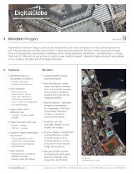
Initial Project Setup<br />
1. Start OrthoEng<strong>in</strong>e and click ‘New’ on the File menu to start a new project.<br />
2. Give your project a ‘Filename’, ‘Name’ and ‘Description’.
3. Select ‘Optical Satellite Model<strong>in</strong>g’ as the Math Model<strong>in</strong>g Method.<br />
4. Under Options, select ‘Rational Functions’. After accept<strong>in</strong>g this panel you will be<br />
prompted to set up the projection <strong>in</strong>formation for the output files, the output pixel<br />
spac<strong>in</strong>g, and the projection <strong>in</strong>formation of GCPs. Enter the appropriate projection<br />
<strong>in</strong>formation for your project.<br />
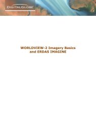
Stitch Images (optional)*<br />
Fig.1. Project Set Up<br />
<strong>WorldView</strong>-1 and <strong>WorldView</strong>-2 data is delivered <strong>in</strong> Geotiff 1.0, NITF 2.0, and NITF 2.1 formats,<br />
which are fully supported by Geomatica OrthoEng<strong>in</strong>e v10.3. Ortho Ready Stereo data <strong>from</strong><br />
<strong>DigitalGlobe</strong> is also delivered with a number of support files (IMD, RPB, STE, TIL and XML).<br />
Please note that these support files should be located <strong>in</strong> the same directory as the image data<br />
while read<strong>in</strong>g the data. Depend<strong>in</strong>g upon your media delivery method, you may have to copy or<br />
extract your data to your hard disk.<br />
1. Stitch the image tiles that conta<strong>in</strong> an R1C1 and R2C1 by ‘Stitch Image Tiles with RPC’<br />
under ‘Utilities’ menu. Stitch comb<strong>in</strong>es different RPC files <strong>in</strong> to a s<strong>in</strong>gle RPC for the<br />
entire stitched image. The image will get converted <strong>in</strong>to .PIX format.<br />
* If you have tiled Stereo imagery <strong>from</strong> <strong>DigitalGlobe</strong> it is best to perform this process.
Fig.2. Stitch Image Tiles with RPC<br />
2. After successful completion, software will prompt to add the stitched image to the<br />
project. Select OK to cont<strong>in</strong>ue with the project.<br />
3. The stereo pair of the Worldview-2 might be delivered <strong>in</strong> separate tiles as well. In that<br />
case, stitch the stereo image and add it to the project as well. Otherwise, add .TIFF file<br />
to the project and cont<strong>in</strong>ue to the next step. The project would then consist of two files<br />
(two .PIX files if stereo images were stitched and added to the project; one .TIFF file and<br />
the other .PIX file if only the ma<strong>in</strong> image were <strong>in</strong> tiles).<br />
Collect GCPs and Tie Po<strong>in</strong>ts<br />
At this po<strong>in</strong>t you can proceed right to the <strong>DEM</strong> From Stereo process<strong>in</strong>g step if you do not have<br />
GCPs. In this exercise we are not us<strong>in</strong>g GCPs. The model will be computed based on the<br />
supplied RPCs. If you do have a few GCPs, you can proceed to the GCP collection stage to add<br />
these to your project. The model will be updated automatically, and you can review these GCPs<br />
<strong>in</strong> the residual report panel.
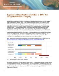
<strong>DEM</strong> <strong>from</strong> Stereo: Generate Epipolar Images<br />
1. When ‘User Select’ is chosen as ‘Epipolar selection’, selection of exact left and right<br />
image does not matter. Just select any image as ‘Left Image’ and other image will be<br />
added as the right image.<br />
2. Make sure to select the image under ‘Right Image’ box and click on ‘Add Epipolar<br />
Pairs to Table’ to record the pair(s) under List of ‘Epipolar Pairs’. If ‘User Select’ is<br />
chosen, repeat the steps until all stereo pairs are recorded.<br />
3. In ‘Down Sample Factor’ put the number of image pixels and l<strong>in</strong>es required to calculate<br />
one epipolar image pixel.<br />
Fig.3. Generate Epipolar Image
4. In ‘Down sample filter’, click the method used to determ<strong>in</strong>e the value of the epipolar<br />
image pixel when the Down Sample Factor is greater than 1. Select one of the follow<strong>in</strong>g:<br />
‘Average’ to assign the average image pixel value to the epipolar image pixel. The average<br />
is obta<strong>in</strong>ed by add<strong>in</strong>g the image pixel values that will become one epipolar image pixel<br />
and divid<strong>in</strong>g that value by the number of image pixels used <strong>in</strong> the sum.<br />
‘Median’ to assign the median value of the image pixels to the epipolar image pixel. The<br />
median is obta<strong>in</strong>ed by rank<strong>in</strong>g the image pixels that will become one epipolar image<br />
pixel accord<strong>in</strong>g to brightness. The median is the middle value of those image pixels,<br />
which is then assigned to the epipolar image pixel.<br />
‘Mode’ to assign the mode value of the image pixels to the epipolar pixel. The mode is the<br />
image pixel value that occurs the most frequently among the image pixels that will<br />
become one epipolar image pixel.<br />
5. Check off the epipolar pairs under the ‘Select’ column and then click on ‘Generate Pairs’.<br />
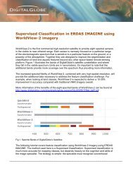
Extract <strong>DEM</strong><br />
1. Under the <strong>DEM</strong> <strong>from</strong> Stereo process<strong>in</strong>g step, select ‘Extract <strong>DEM</strong> Automatically’<br />
button.<br />
2. In ‘Select’ column, check off the epipolar pair <strong>from</strong> which the <strong>DEM</strong> will be extracted<br />
3. Under the ‘Epipolar <strong>DEM</strong> <strong>Extraction</strong> Options’: Enter ‘M<strong>in</strong>imum’ and ‘Maximum’<br />
elevation values. This elevation range is used to estimate the search area for the<br />
correlation. This would <strong>in</strong>crease the speed of the correlation and reduce errors.<br />
Note: If the result<strong>in</strong>g <strong>DEM</strong> conta<strong>in</strong>s failed areas on peaks or valleys, then try <strong>in</strong>creas<strong>in</strong>g<br />
the range.<br />
4. For ‘Failure’ value, enter the value used to represent the failed pixels <strong>in</strong> the output <strong>DEM</strong>.<br />
The default is set to be -100<br />
5. Enter a ‘Background value’ to represent “No Data” pixels that lie outside the <strong>DEM</strong>.<br />
These pixels are dist<strong>in</strong>guished so that they would not be mistaken for elevation values.<br />
The default value is -150.<br />
6. For ‘<strong>DEM</strong> Detail’, specify the level of detail desired for the output <strong>DEM</strong>. Low detail<br />
<strong>in</strong>dicates that the process stops dur<strong>in</strong>g the coarse correlation phase of aggregated
pixels. High detail would mean that the process cont<strong>in</strong>ues until correlation is performed<br />
on images at full resolution.<br />
7. In the ‘Output <strong>DEM</strong> channel type’, enter 32 bit real.<br />
8. Select the desired ‘Pixel Sampl<strong>in</strong>g Interval’, or sampl<strong>in</strong>g frequency. This parameter<br />
controls the size of the pixel <strong>in</strong> the output <strong>DEM</strong> relative to the <strong>in</strong>put images. The higher<br />
the number specified, the larger the <strong>DEM</strong> pixel will be and the faster the <strong>DEM</strong> is<br />
processed.<br />
9. Under the ‘Geocoded <strong>DEM</strong>’’ section, select ‘Create Geocoded <strong>DEM</strong>’ to geocode and<br />
merge the epipolar <strong>DEM</strong>s. However if the <strong>DEM</strong> is to be edited prior to geocod<strong>in</strong>g, leave<br />
this option unselected. If the option is selected, enter a file name for output <strong>DEM</strong>.<br />
10. Click on ‘Extract <strong>DEM</strong>’ button.<br />
Fig.4. Automatic <strong>DEM</strong> <strong>Extraction</strong> Panel
Edit <strong>DEM</strong><br />
The generated <strong>DEM</strong> may conta<strong>in</strong> pixels and/or areas of failed or <strong>in</strong>correct values. It is possible<br />
to edit the <strong>DEM</strong> to smooth out the irregularities and create a more pleas<strong>in</strong>g output.<br />
1. The tool to edit <strong>DEM</strong>s can be accessed <strong>in</strong> ‘OrthoEng<strong>in</strong>e > <strong>DEM</strong> <strong>from</strong> Stereo ><br />
Manually Edit Generated <strong>DEM</strong>’. Click on this button, Focus will open and the <strong>DEM</strong><br />
Edit<strong>in</strong>g panel will be displayed.<br />
In the <strong>DEM</strong> Edit<strong>in</strong>g panel:<br />
2. For ‘Input’, browse to the <strong>DEM</strong> that was created <strong>from</strong> <strong>DEM</strong> <strong>Extraction</strong> step and select<br />
the layer that conta<strong>in</strong>s the <strong>DEM</strong>.<br />
3. Under ‘<strong>DEM</strong> Special Values’, enter the failed and background values of the <strong>DEM</strong>.<br />
4. As ‘Output’, select ‘Save’ and specify an output file name. Enter <strong>in</strong> a layer name as<br />
well. Enable ‘Load results to <strong>in</strong>put’ if edits are to be done repeatedly to achieve a<br />
cumulative effect on the data.<br />
5. Click on ‘Display saved results’.<br />
‘Masks’ can be used to identify areas that are to be edited. Area fills, filter<strong>in</strong>g and <strong>in</strong>terpolation<br />
will be performed to the area under the mask.<br />
6. In the Mask Operations section of the panel, click on the ‘New Mask Layer’ button.<br />
Then click on the ‘Mask Failed Pixels’ button to generate a bitmap mask over pixels<br />
that have the DN value of failed areas.<br />
Pixel values under the mask can be replaced with a specified value or average based on other<br />
shapes.<br />
7. To replace values, select the method under ‘Fill us<strong>in</strong>g’ and then click Fill. Filters can<br />
also be used to elim<strong>in</strong>ate failed or <strong>in</strong>correct values. Filters can be applied repeatedly or<br />
<strong>in</strong> different comb<strong>in</strong>ations for a cumulative effect. It is also possible to filter areas under<br />
masks.<br />
8. To apply a filter, specify the desired method under ‘Filter<strong>in</strong>g and Interpolation’. Select<br />
the area to be filtered (entire <strong>DEM</strong> or area under mask) and click ‘Apply’.
Exam<strong>in</strong>e Results<br />
Fig.5. <strong>DEM</strong> Edit<strong>in</strong>g Panel<br />
Exam<strong>in</strong>e the <strong>DEM</strong> <strong>in</strong> Focus and cont<strong>in</strong>ue edit<strong>in</strong>g if necessary. Bad results <strong>in</strong> the <strong>DEM</strong> can often<br />
be caused by the data, the stereo coverage, the accuracy of the model generated <strong>from</strong> control<br />
po<strong>in</strong>ts, etc. If there are numerous failed areas that cannot be easily corrected us<strong>in</strong>g the <strong>DEM</strong><br />
Edit<strong>in</strong>g Tools, then try return<strong>in</strong>g to OrthoEng<strong>in</strong>e and generat<strong>in</strong>g epipolar images aga<strong>in</strong> or
extract<strong>in</strong>g <strong>DEM</strong> us<strong>in</strong>g different parameters (e.g. <strong>in</strong>crease the down scale factor). The <strong>PCI</strong><br />
Geomatica help files on ‘Apply<strong>in</strong>g Tool Strategies for Common Situations <strong>in</strong> Digital Elevation<br />
Models’ conta<strong>in</strong> more <strong>in</strong>formation about improv<strong>in</strong>g <strong>DEM</strong> output.<br />
For more technical <strong>in</strong>formation on <strong>DigitalGlobe</strong> <strong>Imagery</strong> Products please visit<br />
http://www.digitalglobe.com/resources<br />
For more <strong>in</strong>formation on <strong>PCI</strong> Geomatica and <strong>PCI</strong> Products please visit<br />
http://www.pcigeomatics.com/