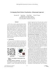
Transfer Functions for Direct Volume Rendering

Transfer Functions for 

Direct Volume Rendering 

Gordon Kindlmann 

gk@cs.utah.edu 

http://www.cs.utah.edu/~gk 

Scientific Computing and Imaging Institute 

School of Computing 

University of Utah 

Contributions: 

Many, as noted

Outline 

1. Transfer Functions: 

what and why 

2. Review of current methods 

3. Ideas for future work

Introduction 

Transfer functions make volume data visible 

by mapping data values to optical properties 

slices: volume rendering: 

8 140 

volume data: 

What and Why

α 

Human Tooth CT 

Transfer Functions (TFs) 

RGB 

RGB(f) 

Simple (usual) case: Map data 

value f to color and opacity 

α(f) 

f 

Shading, 

Compositing… 

Motivation

Optical Properties 

Anything that can be composited with a 

standard graphics operator (“over”) 

• Opacity: “opacity functions” 

• Most important 

• Color 

• Can help distinguish features 

• Emittance 

• Why don’t we use this more often? 

• Phong parameters (k a , k d , k s ) 

• Index of refraction 

What and Why

α 

α 

f 

Alas… 

Setting transfer functions is difficult, 

unintuitive, and slow 

f 

α 

α 

f 

f 

What and Why

TFs as feature detection 

Where’s the edge? 

Result is set of edge pixels: 

v = f (x) 

“ here’s the edge ! ” 

What and Why 

x

α 

(v) 


We are looking in the data value domain, 

not the spatial domain 

v 0 

v 

v = f (x) 

v 0 

What and Why 

“ here’s 

the edge ! ” 

x

v = f (x) 

v = f (x) 

v 0 


“ here’s the edge ! ” 

“ here’s 

the edge ! ” 

x 

x 

What and Why 

Domain of 

the transfer 

function 

does not 

include 

position

Goals 

• Make good renderings easier to come by 

• Make space of TFs less confusing 

• Remove excess “flexibility” 

• Provide one or more of: 

• Information 

• Guidance 

• Semi-automation 

• Automation 

What and Why

Outline 

1. Transfer Functions: what and why 

2. Review of current methods 


Organization 

1.Trial and Error (manual) 

2.Spatial Feature Detection 

3.Image-Centric 

4.Data-Centric 

5.Others 

Current Methods

1. Manually edit 

graph of transfer 

function 

2. Enforces learning 

by experience 

3. Get better with 

practice 

4. Can make terrific 

images 

1. Trial and Error 

Current Methods 

William Schroeder, Lisa Sobierajski Avila, and 

Ken Martin; Transfer Function Bake-off Vis ’00

Organization 





5.Others 

Current Methods


2. Spatial Feature Detection 

Transform TF specification to feature 

detection in the spatial domain 

• extremely flexible 

• different parameter space 

• not exactly transfer functions … 

1. Fang, Biddlecome, Tuceryan (Vis ‘98) 

“Image-based Transfer Function Design…” 

2. Rheingans, Ebert (Vis ’00, TVCG July ’01) 

“Volume Illustration: Non-photorealistic…” 

3. Hladuvka, Gröller (VisSym ’01) “Salient 

Representation of Volume Data”

Traditional Volume Rendering Pipeline 

voxel colors c λ(x i) 

Volume values f 1 (x i ) 

shading classification 

shaded, segmented volume [c λ (x i ), α(x i )] 

resampling and compositing 

(raycasting, splatting, etc.) 

image pixels C λ(u i) 

Volume Illustration 

voxel opacities α(x i ) 

Volume 

Rendering 

3. Spatial Features 

Volume Illustration Rendering Pipeline 

volume values f 1(x i) 

Transfer function 

Volume Illustration Volume Illustration 

color modification opacity modification 

Final volume sample [cλ(x i), α(x i)] 

Feature Enhancement 

• Boundary, silhouette enhancement 

Depth and Orientation Cues 

• Halos, depth cueing 

image pixels Cλ(u i) 

Thanks to Penny Rheingans and David Ebert



Original TF Boundaries (gradient)


Silhouettes Halos 


Blurs distinction between transfer functions and feature detection

Organization 





5.Others 

Current Methods

3. Image-centric 


Specify TFs via the resulting renderings 

• Genetic Algorithms (“Generation of Transfer Functions with 

Stochastic Search Techniques”, He, Hong, et al.: Vis ’96) 

• Design Galleries (Marks, Andalman, Beardsley, et al.: 

SIGGRAPH ’97; Pfister: Transfer Function Bake-off Vis ’00) 

• Thumbnail Graphs + Spreadsheets (“A Graph 

Based Interface…”, Patten, Ma: Graphics Interface ’98; “Image 

Graphs…”, Ma: Vis ’99; Spreadsheets for Vis: Vis ’00, TVCG July ’01) 

• Thumbnail Parameterization (“Mastering Transfer 

Function Specification Using VolumePro Technology”, König, Gröller: 

Spring Conference on Computer Graphics ’01)

Genetic Algorithms 

3. Image-Centric 

Initial stochastic search; refinement can be 

user driven or automated (“fitness functions”) 

“Generation of Transfer 

Functions with Stochastic 

Search Techniques”, He, 

Hong, et al.: Vis ’96

Design Galleries 

Effective method for general class of 


“parameter tweaking” problems 

• Provide convenient GUI to whole parameter 

space (“what’s possible?”) 

• Sampling parameter space: dispersion 

• Organize output images: arrangement 

Inputs: 

Transfer Functions 

Graphics 

Process 

Outputs: 

Images 

Organize Images for easy browsing

VolDG 

(software 

available) 

Marks, 

Andalman, 

Beardsley, et 

al.: SIGGRAPH 

’97; Pfister: 

Transfer 

Function Bakeoff 

Vis ’00 

Design Galleries 

3. Image-Centric

Thumbnail Graphs, Spreadsheets 


Exploration guided by logically connected visual history or spreadsheet 

“A Graph Based Interface for Representing 

Volume Visualization Results”, Patten, Ma: 

Graphics Interface ‘98 

“Visualization Exploration and Encapsulation via 

a Spreadsheet-Like Interface”, Jankun-Kelly, Ma: 

TVCG July 2001

“Mastering 

Transfer 

Function 

Specification 

Using 

VolumePro 

Technology”, 

König, Gröller: 

Spring 

Conference on 

Computer 

Graphics ’01 


Thumbnail Parameterization

Organization 





5.Others 

Current Methods

4. Data-centric 


Specify TF by analyzing volume data itself 

1. Salient Isovalues: 

• Contour Spectrum (Bajaj, Pascucci, Schikore: Vis ’97) 

• Statistical Signatures (“Salient Iso-Surface Detection 

Through Model-Independent Statistical Signatures”, Tenginaki, Lee, 

Machiraju: Vis ’01) 

• Other computational methods (“Fast Detection of 

Meaningful Isosurfaces for Volume Data Visualization”, Pekar, 

Wiemker, Hempel: Vis ’01) 

2. “Semi-Automatic Generation of Transfer 

Functions for Direct Volume Rendering” 

(Kindlmann, Durkin: VolVis ’98; Kindlmann MS Thesis ’99; Transfer 

Function Bake-Off Panel: Vis ‘00)

Salient Isovalues 

4. Data-Centric 

What are the “best” isovalues for extracting 

the main structures in a volume dataset? 

Contour Spectrum (Bajaj, Pascucci, 

Schikore: Vis ’97; Transfer Function 

Bake-Off: Vis ’00) 

• Efficient computation of 

isosurface metrics 

• Area, enclosed volume, 

gradient surface integral, etc. 

• Efficient connected-component 

topological analysis 

• Interface itself concisely 

summarizes data

Contour Spectrum 

4. Data-Centric

Statistical Signatures 

• Localized k-order central moments 

• At each position P in volume, compute … 

• LM : mean over local window W 

• m k : local higher order moment (LHOM) 

Example: m 3 

(Thanks to Shiva Tenginaki, 

Jinho Lee, Raghu Machiraju) 

4. Data-Centric

• Small window 

Boundary Model 

• Boundary if |C 1 – C 2| > 0 

• Binomial distribution of 

materials 

w 

• Extrema and zero-crossings 

of moments and cummulants 

are influenced by presence of 

boundaries 

C 1 

n 


P 

w 

m 

C 2


Moments + Cummulants 

m 2 m 3 m 4 

Skew Kurtosis

Scatterplots 

skew vs. value 

4. Data-Centric

Scatterplots 

4. Data-Centric

Tooth renderings 

4. Data-Centric

Other Computational Methods 

“Fast Fast Detection of Meaningful Isosurfaces for Volume 

Data Visualization”, 

Visualization , Pekar et al.: al. : Vis ‘01 01 


Integral of gradient magnitude over isosurface 

• High for isovalues of strong boundaries 

• Can be computed with divergence theorem: 

Integral of vector field over surface is same 

as integral of divergence in the interior 

• Application of classical vector calc 

• Rapid computation with Laplacian-weighted 

histograms


gray value histogram total gradient 

isosurface area isosurface curvature 


mean gradient total gradient divided by curvature 

Pekar et al. “Fast Fast Detection of Meaningful Isosurfaces for Volume Data Visualization“, Visualization , Vis ‘01 01



MEAN gradient combined with the opacity transfer function 

Pekar et al. “Fast Fast Detection of Meaningful Isosurfaces for Volume Data Visualization“, Visualization , Vis ‘01 01

“Semi-Automatic …” 


Reasoning: 

• TFs are volume-position invariant 

• Histograms “project out” position 

• Interested in boundaries between materials 

• Boundaries characterized by derivatives 

Make 3D histograms of value, 1 st , 2 nd deriv. 

By (1) inspecting and 

(2) algorithmically analyzing 

histogram volume, we can 

create transfer functions

Derivative relationships 


Edges at maximum 

of 1 st derivative or 

zero-crossing of 2 nd

Ideal 

Turbine Blade 

Engine Block 

(1) Scatterplots 


Project histogram 

volume to 2D 

scatterplots 

• Visual summary 

• Interpreted for 

TF guidance 

• No reliance on 

boundary model 

at this stage

x 

z 

(2) Analysis 

Volume Graphics Distance Map 

(x,y,z) 

d 

y 

New Distance Map 

v 

0 255 

x 

y 

z 

3D position 

v 

data value 

d 


Signed 

distance to 

boundary

(2) New Distance Maps 

v = f (x) 

v 0 

• Supports 2D distance map: 

x 

d(v) 

d(v,g); g = gradient magnitude 

• Produced automatically from 

histogram volume via boundary model 

v 0 


v

Automatically 

generated from 

histogram volume 

distance function: 

d(v) 

data value: v 

(2) Whole process 

Created by 

user 

“distance”: x 

opacity function: 

α(v) 

opacity: a 

• Opacity function: α(v) = b(d(v)) 

α = b(x) 

-2 -1 0 1 2 

boundary emphasis 

function: 

b(x) 

α(v,g) = b(d(v,g)) 


x

v 

x 

Results: CT Head 

CT head slice 

α 

d(v) 

f -- f ’ f -- f ’’ 

4. Data-Centric

v 

Results: CT Head 

x 

α v 

x 

α 

4. Data-Centric

Results: Tooth 

b(x) 

-2 -1 0 1 2 

x 


Boundary emphasis function 

simple to set 

α(v) = b(d(v))

Tooth: 2D transfer function 

Detected 4 distinct boundaries between 4 materials 

d(v,g) 

• Pulp 

• Background 

• Dentine 

• Enamel 

- 

0 + 


White regions in 

colormapped 2D distance 

function plot are boundary 

centers 

Color transfer function

Mostly accurate 

isolation of all 

material 

boundaries 

2D Opacity Functions 

4. Data-Centric

Organization 





5.Others 

Current Methods

5. Other methods 

• New domains: curvature 

• New kinds of interaction

Curvature 

“Curvature-Based Transfer Functions for Direct Volume 

Rendering”, Hladuvka, König, Gröller: SCCG ’00 

• Uses 2D space of κ1 and κ2 : 

principal curvatures of isosurface 

at a given point 

• Graphically indicates aspects of 

local shape 

• Specification is simple 

Other Methods

Different Interaction 

Other Methods 

“Interactive Volume Rendering Using Multi-Dimensional Transfer 

Functions and Direct Manipulation Widgets” Kniss, Kindlmann, Hansen: Vis ’01 

• Make things opaque by pointing at them 

• Uses 3D transfer functions (value, 1 st , 2 nd derivative) 

• “Paint” into the transfer function domain

enamel / 

background 

3D Transfer Function 

Motivation 

dentin / background dentin / enamel dentin / pulp 

3D transfer functions allow 

• easier boundary selection 

• accurate boundary visualization

Outline 

1. Transfer Functions: what and why 

2. Current Methods 


Different domains, ranges 

• Time-varying data (“A Study of Transfer Function Generation for 

Time-Varying Volume Data”, Jankun-Kelly, Ma: Volume Graphics ’01) 

• Multi-dimensional TFs expressive and powerful 

• Leverage current techniques for ease of use 

• 2D opacity functions: let’s use them! 

• Marc Levoy’s 1988 CG+A Paper 

Ranges: Emitance, textures, what else? 

Future Work

• Variations on the histogram volume: 

– Different quantities, assumptions, 

models, analysis? 

• Histograms/scatterplots entirely loose 

spatial information 

Other directions 

– Any way to keep some of it? 

– Can TFs have volume position in 

domain? 

Future Work

Other directions 

Future Work 

• Image-centric methods have a certain 

appeal 

– Any way to steer and constrain them more 

effectively? 

– Image-space analysis of TF fitness? 

• What kinds of tools do we really want? 

– Analytical vs. expressive; 

simplifying vs. honest? 

– What is the proper role for human 

experimentation?

Questions?

Transfer Functions for Direct Volume Rendering

Create successful ePaper yourself

Delete template?

Save as template?