Calculation of short-circuit currents - Schneider Electric

Collection Technique .......................................................................... 

Cahier technique no. 158 

Calculation of short-circuit 

currents 

Building a New Electric World 

B. de Metz-Noblat 

F. Dumas 

C. Poulain

"Cahiers Techniques" is a collection of documents intended for engineers 

and technicians, people in the industry who are looking for more in-depth 

information in order to complement that given in product catalogues. 

Furthermore, these "Cahiers Techniques" are often considered as helpful 

"tools" for training courses. 

They provide knowledge on new technical and technological developments 

in the electrotechnical field and electronics. They also provide better 

understanding of various phenomena observed in electrical installations, 

systems and equipment. 

Each "Cahier Technique" provides an in-depth study of a precise subject in 

the fields of electrical networks, protection devices, monitoring and control 

and industrial automation systems. 

The latest publications can be downloaded from the Schneider Electric internet 

web site. 

Code: http://www.schneider-electric.com 

Section: Press 

Please contact your Schneider Electric representative if you want either a 

"Cahier Technique" or the list of available titles. 

The "Cahiers Techniques" collection is part of the Schneider Electric’s 

"Collection technique". 

Foreword 

The author disclaims all responsibility subsequent to incorrect use of 

information or diagrams reproduced in this document, and cannot be held 

responsible for any errors or oversights, or for the consequences of using 

information and diagrams contained in this document. 

Reproduction of all or part of a "Cahier Technique" is authorised with the 

compulsory mention: 

"Extracted from Schneider Electric "Cahier Technique" no. ....." (please 

specify).

no. 158 

Calculation of short-circuit 


Benoît de METZ-NOBLAT 

Graduate Engineer from ESE (Ecole Supérieure d’Electricité), he 

worked first for Saint-Gobain, then joined Schneider Electric in 1986. 

He is now a member of the Electrical Networks competency group 

that studies electrical phenomena affecting power system operation 

and their interaction with equipment. 

Frédéric DUMAS 

After completing a PhD in engineering at UTC (Université de 

Technologie de Compiègne), he joined Schneider Electric in 1993, 

initially developing software for electrical network calculations in the 

Research and Development Department. Starting in 1998, he led a 

research team in the field of industrial and distribution networks. 

Since 2003, as a project manager, he has been in charge of the 

technical development of electrical distribution services. 

Christophe POULAIN 

Graduate of the ENI engineering school in Brest, he subsequented 

followed the special engineering programme at the ENSEEIHT 

institute in Toulouse and completed a PhD at the Université Pierre et 

Marie Curie in Paris. He joined Schneider Electric in 1992 as a 

research engineer and has worked since 2003 in the Electrical 

Networks competency group of the Projects and Engineering Center. 

ECT 158 updated September 2005

Lexicon 

Cahier Technique Schneider Electric n° 158 / p.2 

Abbreviations 

BC Breaking capacity. 

MLVS Main low voltage switchboard. 

Symbols 

A Cross-sectional area of conductors. 

α Angle between the initiation of the 

fault and zero voltage. 

c Voltage factor. 

cos ϕ Power factor (in the absence of 

harmonics). 

e Instantaneous electromotive force. 

E Electromotive force (rms value). 

ϕ Phase angle (current with respect to 

voltage). 

i Instantaneous current. 

iac Alternating sinusoidal component of 

the instantaneous current. 

idc Aperiodic component of the 

instantaneous current. 

ip Maximum current (first peak of 

the fault current). 

I Current (rms value). 

Ib Short-circuit breaking current 

(IEC 60909). 

Ik Steady-state short-circuit current 

(IEC 60909). 

Ik" Initial symmetrical short-circuit current 

(IEC 60909). 

Ir Rated current of a generator. 

Is Design current. 

Isc Steady-state short-circuit current 

(Isc3 = three-phase, 

Isc2 = phase-to-phase, etc.). 

λ Factor depending on the saturation 

inductance of a generator. 

k Correction factor (NF C 15-105) 

K Correction factor for impedance 

(IEC 60909). 

κ Factor for calculation of the peak shortcircuit 

current. 

Ra Equivalent resistance of the upstream 

network. 

RL Line resistance per unit length. 

Sn Transformer kVA rating. 

Scc Short-circuit power 

tmin Minimum dead time for short-circuit 

development, often equal to the time 

delay of a circuit breaker. 

u Instantaneous voltage. 

usc Transformer short-circuit voltage in %. 

U Network phase-to-phase voltage with 

no load. 

Un Network nominal voltage with load. 

x Reactance, in %, of rotating machines. 

Xa Equivalent reactance of the upstream 

network. 

XL Line reactance per unit length. 

Xsubt Subtransient reactance of a generator. 

Z (1) 

Z(2) 

Posititve-sequence 

impedance 

Negative-sequence 

impedance 

Zero-sequence impedance 

Line impedance. 

of a network 

or an 

element. 

Z(0) 

ZL Zsc Network upstream impedance for a 

three-phase fault. 

Zup Equivalent impedance of the upstream 

network. 

Subscripts 

G Generator. 

k or k3 3-phase short circuit. 

k1 Phase-to-earth or phase-to-neutral 

short circuit. 

k2 Phase-to-phase short circuit. 

k2E / kE2E Phase-to-phase-to-earth short circuit. 

S Generator set with on-load tap 

changer. 

SO Generator set without on-load tap 

changer. 

T Transformer.

Summary 

Calculation of short-circuit currents 

In view of sizing an electrical installation and the required equipment, as 

well as determining the means required for the protection of life and 

property, short-circuit currents must be calculated for every point in the 

network. 

This “Cahier Technique” reviews the calculation methods for short-circuit 

currents as laid down by standards such as IEC 60909. It is intended for 

radial and meshed low-voltage (LV) and high-voltage (HV) circuits. 

The aim is to provide a further understanding of the calculation methods, 

essential when determining short-circuit currents, even when computerised 

methods are employed. 

1 Introduction p. 4 

1.1 The main types of short-circuits p. 5 

1.2 Development of the short-circuit current p. 7 

1.3 Standardised Isc calculations p. 10 

1.4 Methods presented in this document p. 11 

1.5 Basic assumptions p. 11 

2 Calculation of Isc by 2.1 Isc depending on the different types of short-circuit p. 12 

the impedance method 

2.2 Determining the various short-circuit impedances p. 13 

2.3 Relationships between impedances at the different 

voltage levels in an installation p. 18 

2.4 Calculation example p. 19 

3 Calculation of Isc values in a radial 3.1 Advantages of this method p. 23 

network using symmetrical components 

3.2 Symmetrical components p. 23 

3.3 Calculation as defined by IEC 60909 p. 24 

3.4 Equations for the various currents p. 27 

3.5 Examples of short-circuit current calculations p. 28 

4 Conclusion p. 32 

Bibliography p. 32 

Cahier Technique Schneider Electric n° 158 / p.3

1 Introduction 

HV / LV 

transformer rating 

b Power factor 

b Coincidence factor 

b Duty factor 

b Foreseeable expansion 

factor 

Load 

rating 

b Feeder current 

ratings 

b Voltage drops 


Electrical installations almost always require 

protection against short-circuits wherever there 

is an electrical discontinuity. This most often 

corresponds to points where there is a change 

in conductor cross-section. The short-circuit 

current must be calculated at each level in the 

installation in view of determining the 

characteristics of the equipment required to 

withstand or break the fault current. 

The flow chart in Figure 1 indicates the 

procedure for determining the various shortcircuit 

currents and the resulting parameters for 

the different protection devices of a low-voltage 

installation. 

In order to correctly select and adjust the 

protection devices, the graphs in Figures 2, 3 

Conductor characteristics 

b Busbars 

v Length 

v Width 

v Thickness 

b Cables 

v Type of insulation 

v Single-core or multicore 

v Length 

v Cross-section 

b Environment 

v Ambient temperature 

v Installation method 

v Number of contiguous circuits 

Upstream Ssc 

u sc(%) 

Isc 

at transformer 

terminals 

Isc 

of main LV switchboard 

outgoers 

Isc 

at head of secondary 

switchboards 

Isc 

at head of final 

switchboards 

Isc 

at end of final 

outgoers 

and 4 are used. Two values of the short-circuit 

current must be evaluated: 

c The maximum short-circuit current, used to 

determine 

v The breaking capacity of the circuit breakers 

v The making capacity of the circuit breakers 

v The electrodynamic withstand capacity of the 

wiring system and switchgear 

The maximum short-circuit current corresponds 

to a short-circuit in the immediate vicinity of the 

downstream terminals of the protection device. 

It must be calculated accurately and used with a 

safety margin. 

c The minimum short-circuit current, essential 

when selecting the time-current curve for circuit 

breakers and fuses, in particular when 

Breaking capacity 

ST and inst. trip setting 






Inst. trip setting 

Main 

circuit breaker 

Main LV 

switchboard 

distribution 

circuit breakers 

Secondary 

distribution 


Final 

distribution 


Fig. 1 : Short-circuit (Isc) calculation procedure when designing a low-voltage electrical installation (ST = short time; Inst. = instantaneous)

v Cables are long and/or the source impedance 

is relatively high (generators, UPSs) 

v Protection of life depends on circuit breaker or 

fuse operation, essentially the case for TN and 

IT electrical systems 

Note that the minimum short-circuit current 

corresponds to a short-circuit at the end of the 

protected line, generally phase-to-earth for LV 

and phase-to-phase for HV (neutral not 

distributed), under the least severe operating 

conditions (fault at the end of a feeder and not 

just downstream from a protection device, one 

transformer in service when two can be 

connected, etc.). 

Note also that whatever the case, for whatever 

type of short-circuit current (minimum or 

maximum), the protection device must clear the 

short-circuit within a time tc that is compatible 

with the thermal stresses that can be withstood 

by the protected cable: 

i2 

2 2 

∫ dt k A 

a5 s 

i (see Fig. 2, 3, and 4) 

t 1 2 

I z1 

1.1 The main types of short-circuits 

I 2 t = k 2 S 2 

Fig. 2 : The I 2 t characteristics of a conductor depending 

on the ambient temperature (1 and 2 represent the rms 

value of the current in the conductor at different 

temperatures θ 1 and θ 2, with θ 1 > θ 2; I z being the limit of 

the permissible current under steady-state conditions). 

Various types of short-circuits can occur in 

electrical installations. 

Characteristics of short-circuits 

The primary characteristics are: 

c Duration (self-extinguishing, transient and 

steady-state) 

I 

where A is the cross-sectional area of the 

conductors and k is a constant calculated on the 

basis of different correction factors for the cable 

installation method, contiguous circuits, etc. 

Further practical information may be found in the 

“Electrical Installation Guide” published by 

Schneider Electric (see the bibliography). 

t 

Fig. 3 : Circuit protection using a circuit breaker. 

t 

Design 

current 

Transient 

overload 

Transient 

overload 

Cable or I 2 t 

characteristic 

I B Ir Iz Isc 

(tri) 

I B Ir Iz 

Circuit breaker 

time-current 

curve 

BC 

Cable or I 2 t 

characteristic 

Fig. 4 : Circuit protection using an aM fuse. 

Furse time-current 

curve 

c Origin 

v Mechanical (break in a conductor, accidental 

electrical contact between two conductors via a 

foreign conducting body such as a tool or an 

animal) 

v Internal or atmospheric overvoltages 


I 

I


v Insulation breakdown due to heat, humidity or 

a corrosive environment 

c Location (inside or outside a machine or an 

electrical switchboard) 

Short-circuits can be: 

c Phase-to-earth (80% of faults) 

c Phase-to-phase (15% of faults). This type of 

fault often degenerates into a three phase fault 

c Three-phase (only 5% of initial faults) 

These different short-circuit currents are 

presented in Figure 5 . 

Consequences of short-circuits 

The consequences are variable depending on 

the type and the duration of the fault, the point in 

the installation where the fault occurs and the 

short-circuit power. Consequences include: 

c At the fault location, the presence of electrical 

arcs, resulting in 

v Damage to insulation 

v Welding of conductors 

v Fire and danger to life 

c On the faulty circuit 

v Electrodynamic forces, resulting in 

- Deformation of the busbars 

- Disconnection of cables 

v Excessive temperature rise due to an increase 

in Joule losses, with the risk of damage to 

insulation 

c On other circuits in the network or in near-by 

networks 

v Voltage dips during the time required to clear 

the fault, ranging from a few milliseconds to a 

few hundred milliseconds 

v Shutdown of a part of the network, the extent 

of that part depending on the design of the 

network and the discrimination levels offered by 

the protection devices 

v Dynamic instability and/or the loss of machine 

synchronisation 

v Disturbances in control / monitoring circuits 

v etc. 

a) Three-phase short-circuit b) Phase-to-phase short-circuit clear of earth 

L3 

L2 

L1 

I " 

k3 

c) Phase-to-phase-to-earth short-circuit d) Phase-to-earth short-circuit 

L3 

L2 

L1 

I " 

k2EL3 

I " 

kE2E 

I " 

k2EL2 

Short-circuit current, 

Partial short-circuit currents in conductors and earth. 

Fig. 5 : Different types of short-circuits and their currents. The direction of current is chosen arbitrarily 

(See IEC 60909). 

L3 

L2 

L1 

L3 

L2 

L1 

I " 

k1 

I " 

k2

1.2 Development of the short-circuit current 

A simplified network comprises a source of 

constant AC power, a switch, an impedance Zsc 

that represents all the impedances upstream of 

the switch, and a load impedance Zs 

(see Fig. 6 ). 

In a real network, the source impedance is made 

up of everything upstream of the short-circuit 

including the various networks with different 

voltages (HV, LV) and the series-connected 

wiring systems with different cross-sectional 

areas (A) and lengths. 

In Figure 6, when the switch is closed and no 

fault is present, the design current Is flows 

through the network. 

When a fault occurs between A and B, the 

negligible impedance between these points 

results in a very high short-circuit current Isc that 

is limited only be impedance Zsc. 

The current Isc develops under transient 

conditions depending on the reactances X and 

the resistances R that make up impedance Zsc: 

2 2 

Zsc = R + X 

In power distribution networks, reactance X = L ϕ 

is normally much greater than resistance R and 

e 

R 

Zsc 

Fig. 6 : Simplified network diagram. 

X 

Fault initiation 

α-ϕ 

ω 

B 

I 

A 

Zs 

i ac = I sin (ωt + α − ϕ) 

the R / X ratio is between 0.1 and 0.3. The ratio 

is virtually equals cos ϕ for low values: 

R 

cos ϕ = 

2 2 

R + X 

However, the transient conditions prevailing 

while the short-circuit current develops differ 

depending on the distance between the fault 

location and the generator. This distance is not 

necessarily physical, but means that the 

generator impedances are less than the 

impedance of the elements between the 

generator and the fault location. 

Fault far from the generator 

This is the most frequent situation. The transient 

conditions are those resulting from the 

application of a voltage to a reactor-resistance 

circuit. This voltage is: 

e = E 2 sin ( ωt + α) 

Current i is then the sum of the two components: 

i = i ac + idc 

c The first (iac) is alternating and sinusoidal 

i ac = Ι 2 sin ( ωt + α−ϕ) where I = E 

Zsc , 

α = angle characterising the difference between 

the initiation of the fault and zero voltage. 

c The second (idc) is an aperiodic component 

- 

idc R 

L t 

= -Ι 2 sin ( α−ϕ ) e . Its initial value 

depends on a and its decay rate is proportional 

to R / L. 

At the initiation of the short-circuit, i is equal to 

zero by definition (the design current Is is 

negligible), hence: 

i = iac + idc = 0 

Figure 7 shows the graphical composition of i as 

the algebraic sum of its two components iac and 

idc i dc = - I sin (α − ϕ) e 

i = i ac + i dc 

R 

L t - 

Fig. 7 : Graphical presentation and decomposition of a short-circuit current occuring far from the generator. 


t

a) Symmetrical 

b) Asymmetrical 


i p 

i 

u 

i 

u 

i dc 

Ir 

The moment the fault occurs or the moment of closing, 

with respect to the network voltage, is characterised by its 

closing angle a (occurrence of the fault). The voltage can 

therefore be expressed as: u = E 2 . sin ( ωt + α ) . 

The current therefore develops as follows: 

E 2 

i = sin t + - - - e 

Z sin 

- R 

L t 

⎡ 

⎤ 

⎢ ( ω α ϕ) ( α ϕ) 

⎥ 

⎢ 

⎥ 

⎣ 

⎦ 

with its two components, one being alternating with a shift 

equal to ϕ with respect to the voltage and the second 

aperiodic and decaying to zero as t tends to infinity. 

Hence the two extreme cases defined by: 

c α = ϕ ≈ π /2, said to be symmetrical (or balanced) 

(see Fig. a ) 

E 2 

The fault current can be defined by: i = sin t 

Z ω 

which, from the initiation, has the same shape as for 

steady state conditions with a peak value E / Z. 

c α = 0, said to be asymmetrical (or unbalanced) 

(see Fig. b ) 

The fault current can be defined by: 

E 2 

- 

i = sin t - + sin e 

Z R 

L t 

⎡ 

⎤ 

⎢ ( ω ϕ) ϕ ⎥ 

⎢ 

⎥ 

⎣ 

⎦ 

Its initial peak value ip therefore depends on ϕ on 

the R / X ≈ cos ϕ ratio of the circuit. 

Fig. 8 : Graphical presentation of the two extreme cases (symmetrical and asymmetrical) for a short-circuit current. 

Figure 8 illustrates the two extreme cases for 

the development of a short-circuit current, 

presented, for the sake of simplicity, with a 

single-phase, alternating voltage. 

R 

The factor e L t − 

is inversely proportional to the 

aperiodic component damping, determined by 

the R / L or R / X ratios. 

The value of ip must therefore be calculated to 

determine the making capacity of the required 

circuit breakers and to define the electrodynamic 

forces that the installation as a whole must be 

capable of withstanding. 

Its value may be deduced from the rms value of 

the symmetrical short-circuit current Ιa using the 

equation: 

ip = κ . r . Ia, where the coefficient κ is 

indicated by the curve in Figure 9 , as a function 

of the ratio R / X or R / L, corresponding to the 

expression: 

R 

−3 

κ = 102 . + 098 . e X 

Fault near the generator 

When the fault occurs in the immediate vicinity of 

the generator supplying the circuit, the variation 

in the impedance of the generator, in this case 

the dominant impedance, damps the short-circuit 

current. 

The transient current-development conditions 

are in this case modified by the variation in the 

electromotive force resulting from the 

shortcircuit. 

For simplicity, the electromotive force is 

assumed to be constant and the internal 

reactance of the machine variable. The 

reactance develops in three stages: 

c Subtransient (the first 10 to 20 milliseconds of 

the fault) 

c Transient (up to 500 milliseconds) 

c Steady-state (or synchronous reactance) 

κ 

2.0 

1.8 

1.6 

1.4 

1.2 

1.0 

0 0.2 0.4 0.6 0.8 1.0 1.2 R/X 

Fig. 9 : Variation of coefficient κ depending on 

R / X or R / L (see IEC 60909).

Note that in the indicated order, the reactance 

acquires a higher value at each stage, i.e. the 

subtransient reactance is less than the transient 

reactance, itself less than the synchronous 

reactance. The successive effect of the three 

reactances leads to a gradual reduction in the 

short-circuit current which is the sum of four 

components (see Fig. 10 ): 

a) 

c The three alternating components (subtransient, 

transient and steady-state) 

c The aperiodic component resulting from the 

development of the current in the circuit (inductive) 

This short-circuit current i(t) is maximum for a 

closing angle corresponding to the zero-crossing 

of the voltage at the instant the fault occurs. 

0 t (s) 

b) 0 t (s) 

c) 

0 t (s) 

d) 0 t (s) 

e) 

0.1 

0 t (s) 

Subtransient Transient Steady-state 

Fig. 10 : Total short-circuit current isc (e), and contribution of its components: 

a) subtransient reactance = X”d 

b) transient reactance = X’d 

c) synchronous reactance = Xd d) aperiodic component. 

Note that the decrease in the generator reactance is faster than that of the aperiodic component. This is a rare 

situation that can cause saturation of the magnetic circuits and interruption problems because several periods 

occur before the current passes through zero. 

0.3 

0.5 


1.3 Standardised Isc calculations 


It is therefore given by the following expression: 

it E 

X X e 

X X e 

t 

X 

E 

X e 

() = 

⎡⎛ 

1 1 ⎞ '' 

t/ T ⎛ ⎞ ' ⎤ 

− 1 1 d −t/ T 1 2 

d −t/ 

T 

2 ⎢ 

a 

⎜ '' − ' ⎟ + ⎜ ' − ⎟ + ⎥cos 

ω − '' 

⎣⎢ 

⎝ d d⎠ 

⎝ d d ⎠ 

d ⎦⎥ 

d 

Where: 

c In LV power distribution and in HV applications, 

E: Phase-to-neutral rms voltage across the however, the transient short-circuit current is often 

generator terminals 

used if breaking occurs before the steady-state 

X" d: Subtransient reactance 

X' d: Transient reactance 

Xd: Synchronous (steady-state) reactance 

T" d: Subtransient time constant 

T' d: Transient time constant 

Ta: Aperiodic time constant 

stage, in which case it becomes useful to use the 

short-circuit breaking current, denoted Ib, which 

determines the breaking capacity of the timedelayed 

circuit breakers. Ib is the value of the 

short-circuit current at the moment interruption is 

effective, i.e. following a time t after the beginning 

of the short-circuit, where t = tmin. Time tmin Practically speaking, information on the 

(minimum time delay) is the sum of the minimum 

development of the short-circuit current is not operating time of a protection relay and the shortest 

essential: 

opening time of the associated circuit breaker, i.e. 

c In a LV installation, due to the speed of the the shortest time between the appearance of the 

breaking devices, the value of the subtransient short-circuit current and the initial separation of the 

short-circuit current, denoted I" k , and of the 

maximum asymmetrical peak amplitude ip is 

sufficient when determining the breaking capacities 

of the protection devices and the electrodynamic 

forces 

pole contacts on the switching device. 

Figure 11 presents the various currents of the 

short-circuits defined above. 

i 

Symmetrical 

Asymmetrical 

2r I" k 

ip 

Subtrans. Transient Steady-state 

Fig. 11 : short-circuit currents near a generator (schematic diagram). 

The standards propose a number of methods. 

c Application guide C 15-105, which 

supplements NF C 15-100 (Normes Françaises) 

(low-voltage AC installations), details three 

methods 

v The “impedance” method, used to calculate 

fault currents at any point in an installation with a 

high degree of accuracy. 

This method involves adding the various 

resistances and reactances of the fault loop 

separately, from (and including) the source to 

the given point, and then calculating the 

2r I k 

corresponding impedance. The Isc value is 

finally obtained by applying Ohm’s law: 

Un 

Isc = 

3 ∑ ( Z) 

. 

All the characteristics of the various elements in 

the fault loop must be known (sources and wiring 

systems). 

v The “composition” method, which may be used 

when the characteristics of the power supply are 

not known. The upstream impedance of the 

given circuit is calculated on the basis of an

estimate of the short-circuit current at its origin. 

Power factor cos ϕ≈ R / X is assumed to be 

identical at the origin of the circuit and the fault 

location. In other words, it is assumed that the 

elementary impedances of two successive 

sections in the installation are sufficiently similar 

in their characteristics to justify the replacement 

of vectorial addition of the impedances by 

algebraic addition. This approximation may be 

used to calculate the value of the short-circuit 

current modulus with sufficient accuracy for the 

addition of a circuit. 

v The “conventional” method, which can be used 

when the impedances or the Isc in the 

installation upstream of the given circuit are not 

known, to calculate the minimum short-circuit 

currents and the fault currents at the end of a 

line. It is based on the assumption that the 

voltage at the circuit origin is equal to 80% of the 

rated voltage of the installation during the shortcircuit 

or the fault. 

Conductor reactance is neglected for sizes 

under 150 mm2 . It is taken into account for large 

1.4 Methods presented in this document 

1.5 Basic assumptions 

In this “Cahier Technique” publication, two 

methods are presented for the calculation of 

short-circuit currents in radial networks: 

c The impedance method, reserved primarily for 

LV networks, was selected for its high degree of 

accuracy and its instructive value, given that 

To simplify the short-circuit calculations, a 

number of assumptions are required. These 

impose limits for which the calculations are valid 

but usually provide good approximations, 

facilitating comprehension of the physical 

phenomena and consequently the short-circuit 

current calculations. They nevertheless maintain 

a fully acceptable level of accuracy, “erring” 

systematically on the conservative side. The 

assumptions used in this document are as 

follows: 

c The given network is radial with nominal 

voltages ranging from LV to HV, but not 

exceeding 550 kV, the limit set by standard 

IEC 60909 

c The short-circuit current, during a three-phase 

short-circuit, is assumed to occur simultaneously 

on all three phases 

c During the short-circuit, the number of phases 

involved does not change, i.e. a three-phase 

sizes by increasing the resistance 15% for 

150 mm2 , 20% for 185 mm2 , 25% for 240 mm2 and 30% for 300 mm2 . 

This method is used essentially for final circuits 

with origins sufficiently far from the source. It is 

not applicable in installations supplied by a 

generator. 

c Standard IEC 60909 (VDE 0102) applies to all 

networks, radial or meshed, up to 550 kV. 

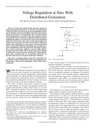
This method, based on the Thevenin theorem, 

calculates an equivalent voltage source at the 

short-circuit location and then determines the 

corresponding short-circuit current. All network 

feeders as well as the synchronous and 

asynchronous machines are replaced in the 

calculation by their impedances (positive 

sequence, negative-sequence and 

zerosequence). 

All line capacitances and the parallel 

admittances of non-rotating loads, except those 

of the zero-sequence system, are neglected. 

virtually all characteristics of the circuit are taken 

into account 

c The IEC 60909 method, used primarily for HV 

networks, was selected for its accuracy and its 

analytical character. More technical in nature, it 

implements the symmetrical-component principle 

fault remains three-phase and a phase-to-earth 

fault remains phase-to-earth 

c For the entire duration of the short-circuit, the 

voltages responsible for the flow of the current 

and the short-circuit impedance do not change 

significantly 

c Transformer regulators or tap-changers are 

assumed to be set to a main position (if the 

short-circuit occurs away far from the generator, 

the actual position of the transformer regulator or 

tap-changers does not need to be taken into 

account 

c Arc resistances are not taken into account 

c All line capacitances are neglected 

c Load currents are neglected 

c All zero-sequence impedances are taken into 

account 


2 Calculation of Isc by the impedance method 

2.1 Isc depending on the different types of short-circuit 


Three-phase short-circuit 

This fault involves all three phases. Short-circuit 

current Isc3 is equal to: 

U / 3 

Ιsc3 

Zcc 

= 

where U (phase-to-phase voltage) corresponds 

to the transformer no-load voltage which is 3 to 

5% greater than the on-load voltage across the 

terminals. For example, in 390 V networks, the 

phase-to-phase voltage adopted is U = 410 V, 

and the phase-to-neutral voltage is 

U / 3 = 237 V. 

Calculation of the short-circuit current therefore 

requires only calculation of Zsc, the impedance 

equal to all the impedances through which Isc 

flows from the generator to the location of the 

Three-phase fault 

Phase-to-phase fault 

Phase-to-neutral fault 

Phase-to-earth fault 

Fig. 12 : The various short-circuit currents. 

Z L 

Z L 

Z L 

Z L 

Z L 

Z L 

Z Ln 

Z L 

Z o 

fault, i.e. the impedances of the power sources 

and the lines (see Fig. 12 ). This is, in fact, the 

“positive-sequence” impedance per phase: 

Zsc = ⎛∑ 

R ⎞ 

⎝ ⎠ ∑ X + ⎛ 2 2 

⎞ 

⎝ ⎠ 

where 

∑R = the sum of series resistances, 

∑X = the sum of series reactances. 

It is generally considered that three-phase faults 

provoke the highest fault currents. The fault 

current in an equivalent diagram of a polyphase 

system is limited by only the impedance of one 

phase at the phase-to-neutral voltage of 

thenetwork. Calculation of Isc3 is therefore 

essential for selection of equipment (maximum 

current and electrodynamic withstand capability). 

V 

U 

V 

V 

Zsc 

Zsc 

Zsc 

Zsc 

Z Ln 

Zsc 

Z o 

Ιsc 

Ιsc 

3 

2 

= 

= 

U / 3 

Zsc 

U 

2 . Zsc 

U / 3 

Ιsc1 

= 

Zsc + ZLn 

Ιsc 

o 

U / 3 

= 

Zsc + Z 

o

Phase-to-phase short-circuit clear of earth 

This is a fault between two phases, supplied with 

a phase-to-phase voltage U. In this case, the 

short-circuit current Isc2 is less than that of a 

three-phase fault: 

U 3 

Ιsc = = Ιsc ≈ 0.86 Ιsc 

2 Zsc 2 

2 3 3 

For a fault occuring near rotating machines, the 

impedance of the machines is such that Isc 2 is 

close to Isc 3. 

Phase-to-neutral short-circuit clear of earth 

This is a fault between one phase and the 

neutral, supplied with a phase-to-neutral voltage 

V = U / 3 

The short-circuit current Isc1 is: 

Ιsc 1 = 

U / 3 

Zsc + ZLn 

2.2 Determining the various short-circuit impedances 

This method involves determining the shortcircuit 

currents on the basis of the impedance 

represented by the “circuit” through which the 

short-circuit current flows. This impedance may 

be calculated after separately summing the 

various resistances and reactances in the fault 

loop, from (and including) the power source to 

the fault location. 

(The circled numbers X may be used to come 

back to important information while reading the 

example at the end of this section.) 

Network impedances 

c Upstream network impedance 

Generally speaking, points upstream of the 

power source are not taken into account. 

Available data on the upstream network is 

therefore limited to that supplied by the power 

distributor, i.e. only the short-circuit power Ssc in 

MVA. 

The equivalent impedance of the upstream 

network is: 

1 Zup = U 

2 

Ssc 

where U is the no-load phase-to-phase voltage 

of the network. 

The upstream resistance and reactance may be 

deduced from Rup / Zup (for HV) by: 

Rup / Zup ≈ 0.3 at 6 kV; 

Rup / Zup ≈ 0.2 at 20 kV; 

In certain special cases of phase-to-neutral 

faults, the zero-sequence impedance of the 

source is less than Zsc (for example, at the 

terminals of a star-zigzag connected transformer 

or of a generator under subtransient conditions). 

In this case, the phase-to-neutral fault current 

may be greater than that of a three-phase fault. 

Phase-to-earth fault (one or two phases) 

This type of fault brings the zero-sequence 

impedance Zo into play. 

Except when rotating machines are involved 

(reduced zero-sequence impedance), the shortcircuit 

current Isco is less than that of a three 

phase fault. 

Calculation of Isco may be necessary, depending 

on the neutral system (system earthing 

arrangement), in view of defining the setting 

thresholds for the zero-sequence (HV) or earthfault 

(LV) protection devices. 

Figure 12 shows the various short-circuit currents. 

Rup / Zup ≈ 0.1 at 150 kV. 

2 2 

As, Xup = Za - Ra , 

Xup 

Zup 

2 

⎛ Rup⎞ 

= 1 - ⎜ ⎟ 

⎝ Zup⎠ 2 Therefore, for 20 kV, 

Xup 

2 

= 1 - ( 0.2) 

= 0. 980 

Zup 

Xup = 0.980 Zup at 20kV, 

hence the approximation Xup ≈ Zup . 

c Internal transformer impedance 

The impedance may be calculated on the basis 

of the short-circuit voltage usc expressed as a 

percentage: 

3 Z u 

2 

U 

T = sc 

, 

100 Sn 

U = no-load phase-to-phase voltage of the 

transformer; 

Sn = transformer kVA rating; 

usc 

= voltage that must be applied to the 

100 

primary winding of the transformer for the rated 

current to flow through the secondary winding, 

when the LV secondary terminals are 

shortcircuited. 

For public distribution MV / LV transformers, the 

values of usc have been set by the European 

Harmonisation document HD 428-1S1 issued in 

October 1992 (see Fig. 13 ) . 

Rating (kVA) of the MV / LV transformer ≤ 630 800 1,000 1,250 1,600 2,000 

Short-circuit voltage u sc (%) 4 4.5 5 5.5 6 7 

Fig. 13 : Standardised short-circuit voltage for public distribution transformers. 



Note that the accuracy of values has a direct 

influence on the calculation of Isc in that an error 

of x % for usc produces an equivalent error (x %) 

for Z T. 

4 In general, RT 150 mm2 ). 

v The reactance per unit length of overhead 

lines, cables and busbars may be calculated as 

X L 15.7 144.44 Log d 

⎡ 

⎛ ⎞ ⎤ 

L = ω = ⎢ + 

⎜ ⎟ 

⎣ 

⎝ r ⎠ ⎥ 

⎦ 

Ssc = 250 MVA 

Ssc = 500 MVA 

0 

500 1,000 1,500 2,000 

Sn 

(kVA) 

Fig. 14 : Resultant error in the calculation of the short-circuit current when the upstream network impedance Zup 

is neglected.

expressed as mΩ / km for a single-phase or 

three-phase delta cable system, where (in mm): 

r= radius of the conducting cores; 

d= average distance between conductors. 

NB : Above, Log = decimal logarithm. 

For overhead lines, the reactance increases 

slightly in proportion to the distance between 

conductors (Log d ⎛ ⎞ 

⎜ ⎟ ), and therefore in 

⎝ t ⎠ 

proportion to the operating voltage. 

7 the following average values are to be used: 

X=0.3 Ω / km (LV lines); 

X=0.4 Ω / km (MV or HV lines). 

Figure 16 shows the various reactance values for 

conductors in LV applications, depending on the 

wiring system (practical values drawn from French 

standards, also used in other European countries). 

The following average values are to be used: 

- 0.08 mΩ /m for a three-phase cable ( ), 

and, for HV applications, between 0.1 and 

0.15 mΩ / m. 

Fig. 16 : Cables reactance values depending on the wiring system. 

8 - 0.09 mΩ / m for touching, single-conductor 

cables (flat or triangular ); 

9 - 0.15 mΩ / m as a typical value for busbars 

( ) and spaced, single-conductor cables 

( ) ; For “sandwiched-phase” busbars 

(e.g. Canalis - Telemecanique), the reactance is 

considerably lower. 

Notes : 

v The impedance of the short lines between the 

distribution point and the HV / LV transformer 

may be neglected. This assumption gives a 

conservative error concerning the short-circuit 

current. The error increases in proportion to the 

transformer rating 

v The cable capacitance with respect to the earth 

(common mode), which is 10 to 20 times greater 

than that between the lines, must be taken into 

account for earth faults. Generally speaking, the 

capacitance of a HV three-phase cable with a 

cross-sectional area of 120 mm 2 is in the order 

Rule Resistitivity Resistivity value Concerned 

(*) (Ω mm2 /m) conductors 

Copper Aluminium 

Max. short-circuit current 

Min. short-circuit current 

ρ0 0.01851 0.02941 PH-N 

c With fuse 

c With breaker 

ρ2 = 1,5 ρ0 

ρ1 = 1,25 ρ0 

0.028 

0.023 

0.044 

0.037 

PH-N 

PH-N (**) 

Fault current for TN and IT ρ1 = 1,25 ρ0 0,023 0,037 PH-N 

systems PE-PEN 

Voltage drop ρ1 = 1,25 ρ0 0.023 0.037 PH-N 

Overcurrent for thermal-stress 

checks on protective conductors 

ρ1 = 1,25 ρ0 0.023 0.037 PH, PE and PEN 

(*) ρ0 = resistivity of conductors at 20°C = 0.01851 Ω mm2 /m for copper and 0.02941 Ω mm2 /m for aluminium. 

(**) N, the cross-sectional area of the neutral conductor, is less than that of the phase conductor. 

Fig. 15 : Conductor resistivity ρ values to be taken into account depending on the calculated short-circuit current 

(minimum or maximum). See UTE C 15-105. 

Wiring system Busbars Three-phase Spaced single-core Touching single 3 touching 3 «d» spaced cables (flat) 

cable cables core cables (triangle) cables (flat) d = 2r d = 4r 

Diagram 

Reactance per unit length, 

values recommended in 

UTE C 15-105 (mΩ/m) 

0.08 0.13 0.08 0.09 0.13 0.13 

Average reactance 

per unit length 

values (mΩ/m) 

0.15 0.08 0.15 0.085 0.095 0.145 0.19 

Extreme reactance 

per unit length 

values (mΩ/m) 

0.12-0.18 0.06-0.1 0.1-0.2 0.08-0.09 0.09-0.1 0.14-0.15 0.18-0.20 

d d 


r


of 1 µF / km, however the capacitive current 

remains low, in the order of 5 A / km at 20 kV. 

c The reactance or resistance of the lines may 

be neglected. 

If one of the values, RL or XL, is low with respect 

to the other, it may be neglected because the 

resulting error for impedance ZL is consequently 

very low. For example, if the ratio between RL and XL is 3, the error in ZL is 5.1%. 

The curves for RL and XL (see Fig. 17 ) may be 

used to deduce the cable cross-sectional areas 

for which the impedance may be considered 

comparable to the resistance or to the 

reactance. 

Examples : 

v First case: Consider a three-phase cable, at 

20°C, with copper conductors. Their reactance 

is 0.08 mΩ / m. The RL and XL curves 

(see Fig. 17) indicate that impedance ZL approaches two asymptotes, RL for low cable 

cross-sectional areas and XL = 0.08 mΩ / m for 

high cable cross-sectional areas. For the low and 

high cable cross-sectional areas, the impedance 

ZL curve may be considered identical to the 

asymptotes. 

The given cable impedance is therefore 

considered, with a margin of error less than 

5.1%, comparable to: 

- A resistance for cable cross-sectional areas 

less than 74 mm2 mΩ/m 

1 

0.8 

0.2 

0.1 

0.08 

0.05 

0.02 

0.01 

10 

Fig. 17 : Impedance Z L of a three-phase cable, at 

20 °C, with copper conductors. 

Fig. 18 : Generator reactance values. in per unit. 

Z L 

X L 

R L 

20 50 100 200 500 1,000 Section S 

2 

(en mm ) 

- A reactance for cable cross-sectional areas 

greater than 660 mm 2 

v Second case: Consider a three-phase cable, at 

20 °C, with aluminium conductors. As above, 

the impedance Z L curve may be considered 

identical to the asymptotes, but for cable crosssectional 

areas less than 120 mm 2 and greater 

than 1,000 mm 2 (curves not shown) 

Impedance of rotating machines. 

c Synchronous generators 

The impedances of machines are generally 

expressed as a percentage, for example: 

x In 

= (where x is the equivalent of the 

100 Isc 

transformer usc). Consider: 

10 Z = x 

100 U 

2 

where 

Sn 

U = no-load phase-to-phase voltage of the 

generator, 

Sn = generator VA rating. 

11 What is more, given that the value of R / X is 

low, in the order of 0.05 to 0.1 for MV and 0.1 to 

0.2 for LV, impedance Z may be considered 

comparable to reactance X. Values for x are 

given in the table in Figure 18 for 

turbogenerators with smooth rotors and for 

“hydraulic” generators with salient poles (low 

speeds). 

In the table, it may seem surprising to see that 

the synchronous reactance for a shortcircuit 

exceeds 100% (at that point in time, Isc < In) . 

However, the short-circuit current is essentially 

inductive and calls on all the reactive power that 

the field system, even over-excited, can supply, 

whereas the rated current essentially carries the 

active power supplied by the turbine 

(cos ϕ from 0.8 to 1). 

c Synchronous compensators and motors 

The reaction of these machines during a 

shortcircuit is similar to that of generators. 

12 They produce a current in the network that 

depends on their reactance in % (see Fig. 19 ). 

c Asynchronous motors 

When an asynchronous motor is cut from the 

network, it maintains a voltage across its 

terminals that disappears within a few 

hundredths of a second. When a short-circuit 

occurs across the terminals, the motor supplies a 

current that disappears even more rapidly, 

according to time constants in the order of: 

Subtransient Transient Synchronous 

reactance reactance reactance 

Turbo-generator 10-20 15-25 150-230 

Salient-pole generators 15-25 25-35 70-120

v 20 ms for single-cage motors up to 100 kW 

v 30 ms for double-cage motors and motors 

above 100 kW 

v 30 to 100 ms for very large HV slipring motors 

(1,000 kW) 

In the event of a short-circuit, an asynchronous 

motor is therefore a generator to which an 

impedance (subtransient only) of 20 to 25% is 

attributed. 

Consequently, the large number of LV motors, 

with low individual outputs, present on industrial 

sites may be a source of difficulties in that it is 

not easy to foresee the average number of 

motors running that will contribute to the fault 

when a short-circuit occurs. Individual calculation 

of the reverse current for each motor, taking into 

account the line impedance, is therefore a 

tedious and futile task. Common practice, 

notably in the United States, is to take into 

account the combined contribution to the fault 

current of all the asynchronous LV motors in an 

installation. 

13 They are therefore thought of as a unique 

source, capable of supplying to the busbars a 

current equal to I start/Ir times the sum of the 

rated currents of all installed motors. 

Other impedances. 

c Capacitors 

A shunt capacitor bank located near the fault 

location will discharge, thus increasing the 

shortcircuit current. This damped oscillatory 

discharge is characterised by a high initial peak 

value that is superposed on the initial peak of the 

shortcircuit current, even though its frequency is 

far greater than that of the network. 

Depending on the timing between the initiation of 

the fault and the voltage wave, two extreme 

cases must be considered: 

v If the initiation of the fault coincides with zero 

voltage, the short-circuit discharge current is 

asymmetrical, with a maximum initial amplitude 

peak 

v Conversely, if the initiation of the fault 

coincides with maximum voltage, the discharge 

current superposes itself on the initial peak of 

the fault current, which, because it is 

symmetrical, has a low value 

It is therefore unlikely, except for very powerful 

capacitor banks, that superposition will result in 

an initial peak higher than the peak current of an 

asymmetrical fault. 

It follows that when calculating the maximum 

short-circuit current, capacitor banks do not need 

to be taken into account. 

However, they must nonetheless be considered 

when selecting the type of circuit breaker. During 

opening, capacitor banks significantly reduce the 

circuit frequency and thus affect current 

interruption. 

c Switchgear 

14 Certain devices (circuit breakers, contactors 

with blow-out coils, direct thermal relays, etc.) 

have an impedance that must be taken into 

account, for the calculation of Isc, when such a 

device is located upstream of the device intended 

to break the given short-circuit and remain closed 

(selective circuit breakers). 

15 For LV circuit breakers, for example, a 

reactance value of 0.15 mΩ is typical, while the 

resistance is negligible. 

For breaking devices, a distinction must be made 

depending on the speed of opening: 

v Certain devices open very quickly and thus 

significantly reduce short-circuit currents. This is 

the case for fast-acting, limiting circuit breakers 

and the resultant level of electrodynamic forces 

and thermal stresses, for the part of the 

installation concerned, remains far below the 

theoretical maximum 

v Other devices, such as time-delayed circuit 

breakers, do not offer this advantage 

c Fault arc 

The short-circuit current often flows through an 

arc at the fault location. The resistance of the arc 

is considerable and highly variable. The voltage 

drop over a fault arc can range from 100 to 300 V. 

For HV applications, this drop is negligible with 

respect to the network voltage and the arc has 

no effect on reducing the short-circuit current. 

For LV applications, however, the actual fault 

current when an arc occurs is limited to a much 

lower level than that calculated (bolted, solid 

fault), because the voltage is much lower. 

16 For example, the arc resulting from a 

shortcircuit between conductors or busbars may 

reduce the prospective short-circuit current by 

20 to 50% and sometimes by even more than 

50% for nominal voltages under 440 V. 

However, this phenomenon, highly favourable in 

the LV field and which occurs for 90% of faults, 

may not be taken into account when determining 

the breaking capacity because 10% of faults take 

place during closing of a device, producing a solid 

Subtransient Transient Synchronous 

reactance reactance reactance 

High-speed motors 15 25 80 

Low-speed motors 35 50 100 

Compensators 25 40 160 

Fig. 19 : Synchronous compensator and motor reactance values, in per unit. 



fault without an arc. This phenomenon should, 

however, be taken into account for the 

calculation of the minimum short-circuit current. 

c Various impedances 

Other elements may add non-negligible 

impedances. This is the case for harmonics 

filters and inductors used to limit the short-circuit 

current. 

They must, of course, be included in 

calculations, as well as wound-primary type 

current transformers for which the impedance 

values vary depending on the rating and the type 

of construction. 

2.3 Relationships between impedances at the different voltage levels in an installation 

Impedances as a function of the voltage 

The short-circuit power Ssc at a given point in 

the network is defined by: 

2 

U 

Ssc = U Ι 3 = 

Zsc 

This means of expressing the short-circuit power 

implies that Ssc is invariable at a given point in 

the network, whatever the voltage. And the 

equation 

U 

Ιsc3 

= implies that all impedances 

3 Zsc 

must be calculated with respect to the voltage at 

the fault location, which leads to certain 

complications that often produce errors in 

calculations for networks with two or more 

voltage levels. For example, the impedance of a 

HV line must be multiplied by the square of the 

reciprocal of the transformation ratio, when 

calculating a fault on the LV side of the 

transformer: 

2 

⎛ U ⎞ 

17 ZBT = Z BT 

HT⎜ 

⎝ U 

⎟ 

HT ⎠ 

A simple means of avoiding these difficulties is 

the relative impedance method proposed by 

H. Rich. 

Calculation of the relative impedances 

This is a calculation method used to establish a 

relationship between the impedances at the 

different voltage levels in an electrical 

installation. 

This method proposes dividing the impedances 

(in ohms) by the square of the network line-toline 

voltage (in volts) at the point where the 

impedances exist. The impedances therefore 

become relative (Z R). 

c For overhead lines and cables, the relative 

resistances and reactances are defined as: 

R 

X 

RCR 

= and X 

2 CR = 

2 with R and X in 

U U 

ohms and U in volts. 

c For transformers, the impedance is expressed 

on the basis of their short-circuit voltages usc and 

their kVA rating Sn: 

1 

ZTR 

= s 

Sn 

u c 

100 

c For rotating machines, the equation is 

identical, with x representing the impedance 

expressed in %. 

1 x 

ZMR 

= 

Sn 100 

c For the system as a whole, after having 

calculated all the relative impedances, the 

shortcircuit power may be expressed as: 

Ssc 

= 

Σ 

1 

from which it is possible to deduce 

ZR the fault current Isc at a point with a voltage U: 

Ιsc 

= 

Σ 

Ssc 1 

= 

3 U 3 U ZR ΣZ R is the composed vector sum of all the 

impedances related to elements upstream of the 

fault. It is therefore the relative impedance of the 

upstream network as seen from a point at U 

voltage. 

Hence, Ssc is the short-circuit power, in VA, at a 

point where voltage is U. 

For example, if we consider the simplified 

diagram of Figure 20 : 

At point A, Ssc = 

Hence, Ssc = 

U 

Z U 

2 

LV 

2 

⎛ ⎞ LV 

T⎜ 

ZL 

⎝ U 

⎟ 

HV ⎠ 

+ 

ZT 

UHV 

1 

Z 

U 2 

L 

LV 2 + 

; 

UHT ZT UBT Z C 

Fig. 20 : Calculating Ssc at point A. 

A

2.4 Calculation example (with the impedances of the power sources, the upstream network 

and the power supply transformers as well as those of the electrical lines) 

Problem 

Consider a 20 kV network that supplies a HV / 

LV substation via a 2 km overhead line, and a 

1 MVA generator that supplies in parallel the 

busbars of the same substation. Two 1,000 kVA 

parallel-connected transformers supply the LV 

busbars which in turn supply 20 outgoers to 

20 motors, including the one supplying motor M. 

All motors are rated 50 kW, all connection cables 

are identical and all motors are running when the 

fault occurs. 

Upstream network 

U1 = 20 kV 

Ssc = 500 MVA 

Overhead line 

3 cables, 50 mm 2 , copper 

length = 2 km 

Generator 

1 MVA 

x subt = 15% 

2 transformers 

1,000 kVA 

secondary winding 237/410 V 

u sc = 5% 

Main LV 

switchboard 

3 bars, 400 mm 2 /ph, copper 

length = 10 m 

Cable 1 

3 single-core cables, 400 mm 2 , 

aluminium, spaced, laid flat, 

length = 80 m 

LV sub-distribution board 

neglecting the length of the busbars 

Cable 2 

3 single-core cables 35 mm 2 , 

copper 3-phase, 

length = 30 m 

Motor 

50 kW (efficiency = 0.9 ; cos ϕ = 0.8) 

x = 25% 

Fig. 21 : Diagram for calculation of Isc3 and ip at points A, B, C and D. 

The Isc 3 and i p values must be calculated at the 

various fault locations indicated in the network 

diagram (see Fig. 21 ), that is: 

c Point A on the HV busbars, with a negligible 

impedance 

c Point B on the LV busbars, at a distance of 

10 meters from the transformers 

c Point C on the busbars of an LV subdistribution 

board 

c Point D at the terminals of motor M 

Then the reverse current of the motors must be 

calculated at C and B, then at D and A. 

3L 

A 

C 

3L 

M 

3L 


D 

10 m 

G 

B


In this example, reactances X and resistances R 

are calculated with their respective voltages in 

Solution 

the installation (see Figure 22 ). The relative 

impedance method is not used. 

Section Calculation Results 

(the circled numbers X indicate where explanations may be found in the preceding text) 

20 kV↓ X (Ω) R (Ω) 

3 

2 

6 

1. upstream network Zup 20 x 10 / 500 x 10 

= ( ) 

Xup = 098 . Zup 

2 0.78 

Rup = 02 . Zup ≈02 

. Xup 0.15 

2. overhead line Xco x . = 04 2 7 0.8 

Rc o x . 

(50 mm 

= 0 018 

2, 000 

50 

6 0.72 

2 ) 

3. generator XG 15 

100 

x 

3 

20 x 10 

10 

2 

6 

10 60 

R G = 01 . XG 

11 6 

20 kV↑ X (mΩ) R (mΩ) 

Fault A 

= ( ) 

2 

1 5 410 

4. transformers ZT = x x 6 

2 100 10 

ZT on LV side 

410 V↓ 

(one 400 mm2 8. cable 1 Xc1 x x 

cable per 

phase) 

. = 015 10 80 

12 

80 

Rc1 = 0. 036 x 

6 7.2 

400 

(35 mm2 10. cable 2 Xc2 x x 

) 

. = 009 10 30 

30 

Rc2 = 0. 023 x 

35 

19.3 

1 

3 5 

XT ≈ ZT 

4.2 

RT = 0.2 XT 

4 0.84 

5. circuit-breaker Xcb = 015 . 

15 0.15 

6. busbars XB = 

-3 

0.15 x 10 x 10 9 1.5 

RB x . 

(one 400 mm 

Fault B 

= 0 023 

10 

400 6 0.57 


0.15 

2 bar per 

phase) 

Fault C 


0.15 

Fault D 

11. motor 50 kW Xm = x 

x 

25 

2 

410 

100 ( 50/ 0. 9 08 . ) 10 3 

Fig. 22 : Impedance calculation. 

Rm = 0.2 Xm 

−3 

−3 

8 2.7 

12 605 

121

I - Fault at A (HV busbars) 

Elements concerned: 1, 2, 3. 

The “network + overhead line” impedance is 

parallel to that of the generator, however the 

latter is much greater and may be neglected: 

X A = 078 . + 08 . ≈ 158Ω . 

RA = 015 . + 072 . ≈ 0.87 Ω 

ZA RA X 

2 2 

= + A ≈ 180Ω . hence 

ΙA = 

3 

20 x 10 

3 x 180 . 

≈ 6,415 A 

IA is the “steady-state Isc” and for the purposes 

of calculating the peak asymmetrical IpA: RA 

= 055 . hence κ =1.2 on the curve in 

XA 

figure 9 and therefore ipA is equal to: 

1.2 x 2 x 6,415 = 10,887 A. 

II - Fault at B (main LV switchboard busbars) 

[Elements concerned: (1, 2, 3) + (4, 5, 6)] 

The reactances X and resistances R calculated 

for the HV section must be recalculated for the 

LV network via multiplication by the square of 

the voltage ratio 17 , i.e.: 

2 

( 410 / 20, 000) = 0. 42 10 -3 hence 

X = ( X 0.42 ) + 42 . + 015 . + 15 . 10 

B A 

[ ] 

X B m . = 651 Ω and 

R = ( R 0.42 ) + 084 . + 057 . 10 

B A 

[ ] 

R B m . = 177 Ω 

These calculations make clear, firstly, the low 

importance of the HV upstream reactance, with 

respect to the reactances of the two parallel 

transformers, and secondly, the non-negligible 

impedance of the 10 meter long, LV busbars. 

ZB RB X 6.75 m 

2 

B 2 

= + = Ω 

ΙB = 

410 

-3 

3 x 6.75 x 10 

≈ 35,070 A 

RB 

XB 

= 027 . hence κ = 1.46 on the curve in 

figure 9 and therefore the peak ipB is equal to: 

1.46 x 2 x 35, 070 ≈ 72,400 A . 

What is more, if the fault arc is taken into 

account (see § c fault arc section 16 ), IB is 

reduced to a maximum value of 28,000 A and a 

minimum value of 17,500 A . 

III - Fault at C (busbars of LV sub-distribution 

board) 

[Elements concerned: (1, 2, 3) + (4, 5, 6) + (7, 8)] 

The reactances and the resistances of the circuit 

breaker and the cables must be added to XB and RB. -3 

XC= ( X B + 015 . + 12) 10 = 1867 . mΩ 

and 

-3 

-3 

-3 

RC= ( R B + 72 . ) 10 = 90 . mΩ 

These values make clear the importance of Isc 

limitation due to the cables. 

ZC RC X m 

2 

C 2 

= + = 20. 7 Ω 

ΙC = 

3 x 

410 

− 

207 . x 10 

≈ 11,400 A 

3 

RC 

XC 

= 048 . hence κ =1.25 on the curve in 

figure 9 and therefore the peak ipC is equal to: 

1.25 x 2 x 11, 400 ≈ 20,200 A 

IV - Fault at D (LV motor) 

[Elements concerned: 

(1, 2, 3) + (4, 5, 6) + (7, 8) + (9, 10)] 

The reactances and the resistances of the circuit 

breaker and the cables must be added to XC and RC. -3 

XD= ( X C + 015 . + 27 . ) 10 = 2152 . mΩ 

and 

-3 

RD= ( R C + 19. 2) 10 = 28. 2 mΩ 

ZD RD X m 

2 

D 2 

= + = 35. 5 Ω 

410 

ΙD = ≈ 6, 

700 A 

-3 

3 x 355 . x 10 

RD 

= 131 . hence κ ≈ 1.04 on the curve in 

XD 

figure 9 and therefore the peak ipD is equal to: 

1.04 x 2 x 6,700 ≈ 9,900 A 

As each level in the calculations makes clear, 

the impact of the circuit breakers is negligible 

compared to that of the other elements in the 

network. 

V - Reverse currents of the motors 

It is often faster to simply consider the motors as 

independent generators, injecting into the fault a 

“reverse current” that is superimposed on the 

network fault current. 

c Fault at C 

The current produced by the motor may be 

calculated on the basis of the “motor + cable” 

impedance: 

−3 

X = ( 605 + 2.7) 10 ≈ 608 mΩ 

M 

-3 

R = ( 121 + 19. 3) 10 ≈ 140 mΩ 

M 

ZM = 624 mΩ hence 

410 

ΙM = ≈ 379 A 

−3 

3 x 624 x 10 

For the 20 motors 

ΙMC = 7, 580 A. 

Instead of making the above calculations, it is 

possible (see 13 ) to estimate the current 

injected by all the motors as being equal to 

(Istart / Ir) times their rated current (98 A), i.e. 

(4.8 x 98) x 20 = 9,400 A. 



This estimate therefore provides conservative 

protection with respect to I MC : 7,580 A. 

On 

the basis of R / X = 0.23 ⇒ κ = 1.51 and 

ipMC = 151 . × 2× 7580 , = 16,200 A 

. 

Consequently, the short-circuit current 

(subtransient) on the LV busbars increases from 

11,400 A to 19,000 A and ipC from 20,200 A to 

36,400 A. 

c Fault at D 

The impedance to be taken into account is 1 / 19th 

of ZM (19 parallel motors), plus that of the cable. 

⎛ 608 ⎞ -3 

XMD 

= ⎜ + 2.7 ⎟ 10 = 34.7 mΩ 

⎝ 19 ⎠ 

⎛ 140 ⎞ -3 

RMD 

= ⎜ + 19.3 ⎟ 10 ≈ 26.7 mΩ 

⎝ 19 ⎠ 

ZMD = 43. 8 m Ω hence 

ΙMD 

= 

410 

= 5, 

400 A 

−3 

3 × 438 . × 10 

giving a total at D of: 

6,700 + 5,400 = 12,100 A rms, and 

ipD ≈ 18,450 A. 

c Fault at B 

As for the fault at C, the current produced by the 

motor may be calculated on the basis of the 

“motor + cable” impedance: 

-3 

XM = ( 605 + 2. 7 + 12) 10 = 620 mΩ 

-3 

R M = ( 121 + 19.3 + 7.2 ) 10 ≈ 147.5 mΩ 

ZM = 637 m Ω hence 

410 

IM 

= 

−3 

3 × 637 × 10 

≈ 

372 A 

For the 20 motors I MB =7,440 A. 

Again, it is possible to estimate the current 

injected by all the motors as being equal to 

4.8 times their rated current (98 A), i.e. 9,400 A. 

The approximation again overestimates the real 

value of I MB. 

Using the fact that R / X = 0.24 = κ = 1.5 

ipMB = 15 . × 2× 7440 , = 15,800 A . 

Taking the motors into account, the short-circuit 

current (subtransient) on the main LV 

switchboard increases from 35,070 A to 

42,510 A and the peak ipB from 72,400 A to 

88,200 A. 

However, as mentioned above, if the fault arc is 

taken into account, IB is reduced between 21.3 

to 34 kA. 

c Fault at A (HV side) 

Rather than calculating the equivalent 

impedances, it is easier to estimate 

(conservatively) the reverse current of the 

motors at A by multiplying the value at B by the 

LV / HV transformation value 17 , i.e.: 

410 

7,440 × = 152.5 A 

3 

20 × 10 

This figure, compared to the 6,415 A calculated 

previously, is negligible 

Rough calculation of the fault at D 

This calculation makes use of all the 

approximations mentioned above (notably 15 

and 16 . 

Σ 

Σ 

Σ 

X = 4.2 + 1.5 + 12 

X = 17.7 m Ω = X' 

R = 7.2 + 19.3 = 26.5 mΩ = R' 

Z'D R'D X' m 

2 

D 2 

= + ≈ 31. 9 Ω 

Ι' D = 

3 x 

410 

-3 

319 . x 10 

≈ 7,430 A 

hence the peak ip' D : 

2 x 7,430 ≈ 10,500 A . 

D 

To find the peak asymmetrical ipDtotal, the above 

value must be increased by the contribution of 

the energised motors at the time of the fault A 

13 i.e. 4.8 times their rated current of 98 A: 

( ) 

10,500+ 4.8 × 98 × 2 × 20 = 23,800 A 

Compared to the figure obtained by the full 

calculation (18,450 A), the approximate method 

allows a quick evaluation with an error remaining 

on the side of safety. 

D

3 Calculation of Isc values in a radial network using 

symmetrical components 

3.1 Advantages of this method 

3.2 Symmetrical components 

Positive-sequence 

I3 (1) 

I2 (1) 

I1 (1) 

ωt 

Calculation using symmetrical components is 

particularly useful when a three-phase network is 

unbalanced, because, due to magnetic 

phenomena, for example, the traditional 

“cyclical” impedances R and X are, normally 

speaking, no longer useable. This calculation 

method is also required when: 

c A voltage and current system is not 

symmetrical (Fresnel vectors with different 

Similar to the Leblanc theorem which states that 

a rectilinear alternating field with a sinusoidal 

amplitude is equivalent to two rotating fields 

turning in the opposite direction, the definition of 

symmetrical components is based on the 

equivalence between an unbalanced threephase 

system and the sum of three balanced threephase 

systems, namely the positivesequence, 

negative-sequence and zerosequence 

(see Fig. 23 ). 

The superposition principle may then be used to 

calculate the fault currents. 

In the description below, the system is defined 

using current Ι1 as the rotation reference, 

where: 

c Ι1 (1) is the positive-sequence component 

c Ι1 is the negative-sequence component 

(2) 

c Ι1 (0) is the zero-sequence component 

and by using the following operator 

I2 (2) 

I1 (2) 

I2 (0) 

ωt 

+ + = 

I3 (2) 

Geometric construction of I1 

I1 

I1 (1) I1 (2) I1 (0) 

Negative-sequence 

ωt 

Zero-sequence 

I1 (0) 

moduli and imbalances exceeding 120°).This is 

the case for phase-to-earth or phase-to-phase 

short-circuits with or without earth connection 

c The network includes rotating machines and/or 

special transformers (Yyn connection, for 

example) 

This method may be used for all types of radial 

distribution networks at all voltage levels. 

a = e = - 1 

2 

j 3 

j 

2 

2π 

3 

and I3. 

+ between I1, I2, 

This principle, applied to a current system, is 

confirmed by a graphical representation 

(see fig. 23). For example, the graphical addition 

of the vectors produces, for, the following result: 

Ι2 = 

2 

a Ι1 + a Ι1 + Ι1 

(1) (2) (3) . 

Currents Ι1and Ι3 may be expressed in the 

same manner, hence the system: 

Ι1 = Ι1 + a Ι1+ Ι1 

(1) (2) (0) 

2 

Ι2 = a Ι1 + a Ι1 + Ι1 

(1) (2) (0) 

2 

(1) (2) (0) 

Ι3 = a Ι1 + a Ι1 + Ι1 

Fig. 23 : Graphical construction of the sum of three balanced three-phase systems (positive-sequence, negative-sequence and zero-sequence). 

I3 (0) 


I1 (0) 

I2 

I1 (1) 

a I1 (2) 

I1 (2) 

a 2 I1 (1) 

I3 

I2 


ωt 


a 2 I1 (2) 

I1 (2) 

I3 

I1 (1) 

I1 (1) 

. 

I1


These symmetrical current components are 

related to the symmetrical voltage components 

by the corresponding impedances: 

Z = V 

Z = V and Z = V 

(1) 

(2) 

(0) 

, 

(1) Ι (2) Ι (0) Ι 

(1) 

(2) 

(0) 

These impedances may be defined from the 

characteristics (supplied by the manufacturers) 

of the various elements in the given electrical 

network. Among these characteristics, we can 

note that Z (2) ≈ Z (1), except for rotating machines, 

whereas Z (0) varies depending on each element 

(see Fig. 24 ). 

For further information on this subject, a detailed 

presentation of this method for calculating solid 

and impedance fault currents is contained in the 

“Cahier Technique” n° 18 (see the appended 

bibliography). 

3.3 Calculation as defined by IEC 60909 

Standard IEC 60909 defines and presents a 

method implementing symmetrical components, 

that may be used by engineers not specialised in 

the field. 

The method is applicable to electrical networks 

with a nominal voltage of less than 550 kV and 

the standard explains the calculation of minimum 

and maximum short-circuit currents. 

The former is required in view of calibrating 

overcurrent protection devices and the latter is 

used to determine the rated characteristics for 

the electrical equipment. 

Procedure 

1- Calculate the equivalent voltage at the fault 

location, equal to c Un / 3 where c is a 

voltage factor required in the calculation to 

account for: 

c Voltage variations in space and in time 

c Possible changes in transformer tappings 

c Subtransient behaviour of generators and 

motors 

Depending on the required calculations and the 

given voltage levels, the standardised voltage 

levels are indicated in Figure 25 . 

2- Determine and add up the equivalent 

positivesequence, negative-sequence and 

zerosequence impedances upstream of the fault 

location. 

3- Calculate the initial short-circuit current using 

the symmetrical components. Practically 

speaking and depending on the type of fault, the 

equations required for the calculation of the Isc 

are indicated in the table in Figure 26 . 

4- Once the rms value of the initial short-circuit 

current (I" k) is known, it is possible to calculate 

the other values: 

ip, peak value, 

Elements 

Transformer 

(seen from secondary winding) 

Z (0) 

No neutral ∞ 

Yyn or Zyn free flux ∞ 

forced flux 10 to 15 X (1) 

Dyn or YNyn X (1) 

Dzn or Yzn 0.1 to 0.2 X (1) 

Machine 

Synchronous ≈ 0.5 Z (1) 

Asynchronous ≈ 0 

Line ≈ 3 Z (1) 

Fig. 24 : Zero-sequence characteristic of the various 

elements in an electrical network. 

Rated Voltage factor c 

voltage for calculation of 

Un Isc max. Isc min. 

LV (100 to 1000 V) 

If tolerance + 6% 1.05 0.95 

If tolerance + 10% 1.1 0.95 

MV and HV 

1 to 550 kV 1.1 1 

Fig. 25 : Values for voltage factor c (see IEC 60909). 

I b, rms value of the symmetrical short-circuit 

breaking current, 

i dc, aperiodic component, 

I k, rms value of the steady-state short-circuit 

current. 

Effect of the distance separating the fault 

from the generator 

When using this method, two different 

possibilities must always be considered: 

c The short-circuit is far from the generator, the 

situation in networks where the short-circuit 

currents do not have a damped, alternating 

component 

This is generally the case in LV networks, except 

when high-power loads are supplied by special 

HV substations; 

c The short-circuit is near the generator 

(see fig. 11), the situation in networks where the 

short-circuit currents do have a damped, 

alternating component. This generally occurs in 

HV systems, but may occur in LV systems when, 

for example, an emergency generator supplies 

priority outgoers.

Type I" k Fault occuring 

of short-circuit General situation far from rotating machines 

Three-phase (any Ze) I" 

= 

k3 

cUn 

Z 

I" 

= 

k3 

cUn 

Z 

Phase-to-phase clear of earth (Ze = ∞) I" 

Phase-to-earth I" 

3 () 1 

The main differences between these two cases 

are: 

c For short-circuits far from the generator 

v The initial (I" k), steady-state (Ik) and breaking 

(Ib) short-circuit currents are equal (I" k = Ik = Ib) v The positive-sequence (Z (1)) and negative 

sequence (Z (2)) impedances are equal (Z (1) = Z (2)) 

Note however that asynchronous motors may also 

add to a short-circuit, accounting for up to 30% of 

the network Isc for the first 30 milliseconds, in 

which case I" k = I k = I b no longer holds true. 

Conditions to consider when calculating the 

maximum and minimum short-circuit 


c Calculation of the maximum short-circuit 

currents must take into account the following 

points 

v Application of the correct voltage factor c 

corresponding to calculation of the maximum 

short-circuit currents 

v Among the assumptions and approximations 

mentioned in this document, only those leading 

to a conservative error should be used 

3 () 1 

In both cases, the short-circuit current depends only on Z (1). which is generally replaced by Z k 

the short-circuit impedance at the fault location, defined by Z k = Rk X 2 

k 2 

Rk is the sum of the resistances of one phase, connected in series; 

Xk is the sum of the reactances of one phase, connected in series. 

+ where: 

cUn 

= 

k2 

Z() 1 + Z( 

2) 

cUn 3 

= 

k1 

Z() 1 + Z( 2) + Z( 

0) 

Phase-to-phase-to-earth 

(Zsc between phases = 0) 

(see fig. 5c) 

I" 

= 

kE2E 

Z Z 

cUn 

+ Z 

3 

Z 

Zi 

+ Z Z 

I" 

() 1 ( 2) ( 2) ( 0) () 1 ( 0) 

I" 

= 

k2 

() 

cUn 

2 Z 1 

cUn 3 

= 

k1 

2 Z() 1 + Z( 

0) 

I" 

I 

" 

kE2E 

cUn Z( 0) − aZ( 

2) 

= 

k2EL2 

Z() 1 Z( 2) + Z( 2) Z( 0) + Z() 1 Z( 

0) I" 

k2EL2 

I 

" 

k2EL3 

= 

2 

( 0) 

− ( 2) 

cUn Z a Z 

Z Z + Z Z + Z Z 

() 1 ( 2) ( 2) ( 0) () 1 ( 0) 

I 

" 

k2EL3 

= 

cUn 

Z + 2 Z 

() 1 ( 0) 

v The resistances per unit length RL of lines 

(overhead lines, cables, phase and neutral 

conductors) should be calculated for a 

temperature of 20 °C 

c Calculation of the minimum short-circuit 

currents requires 

v Applying the voltage factor c corresponding to 

the minimum permissible voltage on the network 

v Selecting the network configuration, and in 

some cases the minimum contribution from 

sources and network feeders, which result in the 

lowest short-circuit current at the fault location 

v Taking into account the impedance of the 

busbars, the current transformers, etc. 

v Considering resistances RL at the highest 

foreseeable temperature 

⎡ 0. 004 ⎤ 

RL 

= + ( e - 20 ° C) x RL20 

⎣ 

⎢ 

1 θ 

° C ⎦ 

⎥ 

where RL20 is the resistance at 20 °C; θe is the 

permissible temperature (°C) for the 

conductor at the end of the short-circuit. 

The factor 0.004 / °C is valid for copper, 

aluminium and aluminium alloys. 


3 

⎛ ⎞ ( ) 

⎜ ⎟ 

⎝ () ⎠ 

= 

− 

cUn 

+ 

Z 0 

a 

Z 1 

Z 2 Z 

() 1 ( 0) 

⎛ ⎞ ( ) 

⎜ ⎟ 

⎝ () ⎠ 

= 

− 

cUn 

+ 

Z 0 

a 

Z 1 

Z 2 Z 

() 1 ( 0) 

Symbol used in this table: c phase-to-phase rms voltage of the three-pase network = Un c short-circuit impedance = Zsc 

c modulus of the short-circuit current = I" k 

c symmetrical impedances = Z (1) , Z (2) , Z (0) 

c earth impedance = Ze. 

Fig. 26 : Short-circuit values depending on the impedances of the given network (see IEC 60909). 

2


Impedance correction factors 

Impedance-correction factors were included in 

IEC 60909 to meet requirements in terms of 

technical accuracy and simplicity when 

calculating short-circuit currents. The various 

factors, presented here, must be applied to the 

short-circuit impedances of certain elements in 

the distribution system. 

c Factor KT for distribution transformers with two 

or three windings 

ZTK = KTZT C 

KT 

= 095 . max 

1+ 0.6xT 

where xT is the relative reactance of the 

transformer: 

x X S 

T T 

U 

rT = 

2 

rT 

and cmax is the voltage factor related to the 

nominal voltage of the network connected to the 

low-voltage side of the network transformer. 

The impedance correction factor must also be 

applied to the transformer negative-sequence 

and zero-sequence impedances when 

calculating unbalanced short-circuit currents. 

Impedances ZN between the transformer 

starpoints and earth must be introduced as 3ZN in the zero-sequence system without a 

correction factor. 

c Factors KG and KS or KSO are introduced when 

calculating the short-circuit impedances of 

generators and power station units (with or 

without on-load tap-changers) 

The subtransient impedance in the positivesequence 

network must be calculated by: 

'' 

ZGK = KGZG= KGRG+ jXd 

( ) 

with R G representing the stator resistance of a 

synchronous machine and the correction factor 

K 

G 

U c 

= n ⋅ max 

'' U 1+ 

x sin ϕ 

rG d rG 

It is advised to use the following values for RGf (fictitious resistance of the stator of a 

synchronous machine) when calculating the 

peak short-circuit current. 

'' 

RGf = 005 . Xdfor 

generators with 

UrG > 1kV et SrG u 100 MVA 

'' 



UrG > 1kV et SrG < 100 MVA 

'' 



UrG i 1000 V 

The impedance of a power station unit with an 

on-load tap-changer is calculated by: 

2 

ZS = KS trZG+ ZTHV 

( ) 

with the correction factor: 

2 2 UnQ 

U 

c 

KS 

= ⋅ rTLV ⋅ max 

2 2 

UrQ 

U 

'' 

rTHV 1+ 

xd−xT sin ϕrG 

U 

and tr 

= rTHV 

UrTLV 

ZS is used to calculate the short-circuit current 

for a fault outside the power station unit with an 

on-load tap-changer. 

The impedance of a power station unit without 

an on-load tap-changer is calculated by: 

2 

ZSO = KSO trZG+ ZTHV 

( ) 

with the correction factor: 

K 

UnQ 

= 

U 1+ 

p 

( ) 

U 

c 

⋅ rTLV ⋅ ± pT 

U 

x 

( ) 1 

max 

'' 

1+ 

sin ϕ 

SO 

rG G rTHV 

d rG 

ZSO is used to calculate the short-circuit current 

for a fault outside the power station unit without 

an on-load tap-changer. 

c Factors KG,S, KT,S or KG,SO, KT,SO are used 

when calculating the partial short-circuit currents 

for a short-circuit between the generator and the 

transformer (with or without an on-load tapchanger) 

of a power station unit 

v Power station units with an on-load tapchanger 

I '' cUrG 

kG = 

3KGS 

, ZG 

where: 

K 

K 

c 

= max 

1+ 

x sin ϕ 

GS , '' 

d rG 

TS , 

c 

= max 

1− 

x sin ϕ 

T rG 

v Power station units without an on-load tapchanger 

I '' cUrG 

kG = 

3KGSO 

, ZG 

where: 

K 

K 

1 

= 

1+ p 

c 

⋅ max 

1+ 

x sin ϕ 

1 

= 

1+ p 

c 

⋅ max 

1−xsin 

ϕ 

GSO , '' 

G d rG 

TSO , 

G T rG

3.4 Equations for the various currents 

Initial short-circuit current (I" k) 

The different initial short-circuit currents I" k are 

calculated using the equations in the table in 

figure 26. 

Peak short-circuit current ip Peak value ip of the short-circuit current In no 

meshed systems, the peak value ip of the shortcircuit 

current may be calculated for all types of 

faults using the equation: 

i p 2 k " 

= κ Ι where 

I" k = is the initial short-circuit current, 

κ = is a factor depending on the R / X and can 

be calculated approximately using the following 

equation (see fig.9) : 

κ = 1.02 + 0.98 e -3R 

X 

Short-circuit breaking current Ib Calculation of the short-circuit breaking current Ib is required only when the fault is near the 

generator and protection is ensured by 

timedelayed circuit breakers. Note that this 

current is used to determine the breaking 

capacity of these circuit breakers. 

This current may be calculated with a fair degree 

of accuracy using the following equation: 

Ib = µ . I" k where: 

where µ = is a factor defined by the minimum 

time delay t min and the I" k / Ir ratio (see Fig. 27 ) 

µ 

1.0 

0.9 

0.8 

0.7 

0.6 

0.5 

0 

1 

which expresses the influence of the 

subtransient and transient reactances, with Ir as 

the rated current of the generator. 

Steady-state short-circuit current Ik The amplitude of the steady-state short-circuit 

current Ik depends on generator saturation 

influences and calculation is therefore less 

accurate than for the initial symmetrical curren I" k. 

The proposed calculation methods produce a 

sufficiently accurate estimate of the upper and 

lower limits, depending on whether the shortcircuit 

is supplied by a generator or a 

synchronous machine. 

c The maximum steady-state short-circuit 

current, with the synchronous generator at its 

highest excitation, may be calculated by: 

Ikmax = λmax Ir 

c The minimum steady-state short-circuit current 

is calculated under no-load, constant (minimum) 

excitation conditions for the synchronous 

generator and using the equation: 

Ikmin = λmin Ir 

λ is a factor defined by the saturated 

synchronous reactance Xd sat. 

The λ max and λ min values are indicated on next 

the page in Figure 28 for turbo-generators and 

in Figure 29 for machines with salient poles 

(series 1 in IEC 60909). 

Minimum the delay t min 

0.02 s 

0.05 s 

0.1 s 

> 0.25 s 

2 3 4 5 6 7 8 9 

Three-phase short-circuit I " k / Ir 

Fig. 27 : Factor µ used to calculate the short-circuit breaking current I b (see IEC 60909). 


λ 

2.4 

2.2 

2.0 

1.8 

1.6 

1.4 

1.2 

1.0 

0.8 

0.6 

0.4 

0.2 

3.5 Examples of short-circuit current calculations 


λ min 

λ max 

Xd sat 

1.2 

1.4 

1.6 

1.8 

2.0 

2.2 

0 

0 1 2 3 4 5 6 7 8 

Three-phase short-circuit current I k " / Ir 

Fig. 28 : Factors λmax and λmin for turbo-generators 

(overexcitation = 1.3 as per IEC 60909). 

Problem 1. A transformer supplied by a 

network 

A 20 kV network supplies a transformer T 

connected to a set of busbars by a cable L 

(see Fig. 30 ). 

It is necessary to calculate, in compliance with 

IEC 60909, the initial short-circuit current I" k and 

the peak short-circuit current ip during a threephase, 

then a phase-to-earth fault at point F1. 

The following information is available: 

c The impedance of the connection between the 

supply and transformer T may be neglected 

c Cable L is made up of two parallel cables with 

three conductors each, where: 

l = 4 m; 3 x 185 mm2 Al 

ZL = (0.208 + j0.068) Ω/km 

R (0)L = 4.23RL; X (0)L = 1.21XL c The short-circuit at point F1 is assumed to be 

far from any generator 

Solution: 

c Three-phase fault at F1 

v Impedance of the supply network (LV side) 

cQUnQ U 

ZQt 

= × rTLV 

m 

kQ UrTHV 

⎛ ⎞ 

⎜ ⎟ 

⎝ ⎠ 

= 

× 

× 

× 

⎛ 

2 2 

11 20 041⎞ 

⎜ ⎟ = 0 534 

3 I 3 10 ⎝ 20 ⎠ 

'' 

. . 

. Ω 

Failing other information, it is assumed that R 

X 

Q 

Q 

λ 

6.0 

5.5 

5.0 

4.5 

4.0 

3.5 

3.0 

2.5 

2.0 

1.5 

1.0 

0.5 

0 

Fig. 29 : Factors λmax and λmin for generators with 

salient poles (overexcitation = 1.6 as per IEC 60909). 

Fig. 30 

= 01 . , hence: 

λ min 

λ max 

1 2 3 4 5 6 7 8 

Three-phase short-circuit current I k " / Ir 

S rT = 400 kVA 

U rTHV = 20 kV 

U rTLV = 410 V 

U kr = 4% 

P krT = 4.6 kW 

R (0)T / R T = 1.0 

X (0)T / X T = 0.95 

F1 

X d sat 

0.6 

0.8 

1.0 

1.2 

1.7 

2.0 

Supply network 

UnQ = 20 kV 

I " kQ = 10 kA 

T (Dyn5) 

Cable L 

l = 4 m 

U n = 400 V

XQt = 0. 995ZQt = 0. 531 mΩ 

RQt = 01 . XQt = 0053 . mΩ 

ZQt = ( 0. 053 + j0. 531) 

mΩ 

c Impedance of the transformer 

u U 

Z 

m 

S 

R P U 

m 

S 

X Z R m 

Z j m 

x X S 

kr rTLV 

TLV 

rT 

TLV krT 

U 

rTLV 

( ) 

= × = × = 

× 

= = 

rT ( × ) 

TLV TLV TLV 

TLV 

rT 

T T 

rTLV 

= 

2 

2 

4 410 

16 81 

100 100 

3 

400 10 

2 

2 

410 

4 600 

483 

2 

3 

400 10 

= − = 16 10 

= 483+ 1610 

400 

= = 16 10 × 

410 

2 

. Ω 

( ) 

, 

. Ω 

2 2 

. Ω 

( . . ) Ω 

. = 0. 03831 

2 

2 

The impedance correction factor can be calculated as: 

c 

KT 

= 

= 

+ xT 

+ ( × ) 

ZTK KTZTLV j m 

= 

105 

095 . max 

. 

095 . 

0. 975 

1 06 . 1 06 . 003831 . 

= = ( 471 . + 1570 . ) Ω 

c Impedance of the cable 

−3 

ZL = 05 . × ( 0208 . + j0068 . ) × 4 10 = ( 0. 416 + j0. 136) 

mΩ 

c Total impedance seen from point F1 

Zk= ZQt + ZTK + ZL= ( 518 . + 1637 . ) mΩ 

c Calculation of I" k and ip for a three-phase fault 

'' cU . 

I n 105× 400 

k = = 

= 14. 12 kA 

3Zk 

3 × 1717 . 

R Rk 

518 . 

= = = 0. 316 

X X 16. 37 

k 

κ = 102 . + 098 . e = 14 . 

'' 

R 

−3 

X 

ip= κ 2 × Ik 

= 14 . 2 × 1412 . = 27. 96 kA 

c Phase-to-earth fault at F1 

v Determining the zero-sequence impedances 

For transformer T (Dyn5 connection), the manufactures indicates: 

R = R and X = X 

( 0) T T ( 0) T 095 . T 

with the impedance-correction factor KT, the zero-sequence impedance is: 

Z( 0) TK = KT( RT+ j095 . XT) = ( 4712 . + j14. 913) 

mΩ 

For cable L: 

Z( 0) L = ( 423 . RL + 121 . XL) = ( 176 . + j0165 . ) mΩ 

v Calculation of I" k and ip for a phase-to-earth fault 

Z() 1 = Z( 2) 

= ZK= ( 518 . + j1637 . ) mΩ 

Z( 0) = Z( 0) TK + Z( 0) 

L = ( 647 . + j1508 . ) mΩ 

Z() 1 + Z( 2) + Z( 0) 

= ( 16. 83 + j47. 82) 

mΩ 

The initial phase-to-earth short-circuit current can be calculated using the equation below: 

I '' cUn 

3 105 . × 400 3 

k1 

= 

= 

= 14. 35 kA 

Z . 

() 1 + Z( 2) + Z( 

0 50 70 

) 

The peak short-circuit current i p1 is calculated with the factor κ obtained via the positive-sequence: 

ip1= κ 2 × Ik1 = 14 2 × 1435 = 28 41 kA 

'' 

. . . 



Problem 2. A power station unit 

A power station unit S comprises a generator G 

and a transformer T with an on-load tap-changer 

(see Fig. 31 ). 

It is necessary to calculate, in compliance with 

IEC 60909, the initial short-circuit current I’’ k as 

well as the peak ip and steady-state Ikmax shortcircuit 

currents and the breaking short-circuit 

current Ib during a three-phase fault: 

c Outside the power station unit on the busbars 

at point F1 

c Inside the power station unit at point F2 

The following information is available: 

c The impedance of the connection between 

generator G and transformer T may be 

neglected 

c The voltage factor c is assumed to be 1.1 

c The minimum dead time tmin for calculation of 

Ib is 0.1 s 

c Generator G is a cylindrical rotor generator 

(smooth poles) 

c All loads connected to the busbars are passive 

Solution: 


v Impedance of the transformer 

u U 

Z 

S 

R P U 

kr rTHV 

THV 

rT 

THV krT x 

S 

X Z R 

Z j 

rTHV 

15 240 

= × = × = 34 56 

100 100 250 

= = 052 = 

rT 

THV = THV − THV = 

THV = + 

240 

2 2 

. Ω 

2 

2 

. 0. 479 Ω 

2 

2 

250 

2 2 

34. 557 Ω 

( 0. 479 34. 557) 

Ω 

v Impedance of the generator 

'' 2 2 

'' x U 

X d rG 17 21 

d = × = × = 0. 2999 Ω 

100 SrG 

100 250 

'' 

ZG = RG+ jXd= 0. 0025 + j0. 

2999 

ZG 

= 0. 2999 Ω 

Fig. 31 

U nQ = 220 kV 

S rG > 100 MVA, therefore R Gf = 0.05 X" d, hence Z Gf = 0.015 + j0.2999 

2 2 U 

2 2 

nQ U 

c 

KS 

= × rTLV × max 220 21 

11 . 

= × × = 0. 913 

2 2 

UrG 

U 

'' 

2 2 

rTHV 1+ 

xd−x + − × 

T sin ϕrG 

21 240 1 017 . 0. 15 0. 6258 

⎛ 2 

2 

⎛ 240⎞ 

⎞ 

ZS = KS( trZG+ ZTHV) = 0. 913 ⎜⎜ 

⎟ × ( 0. 0025 + j0. 2999) + ( 0. 479 + j34. 

557) 

⎝⎝ 

21 ⎠ 

⎟ 

⎠ 

ZS= 0. 735 + j67. 

313 (ZSf = 2.226 + j67.313 if we consider ZGf (to calculate ip)) 

'' cUnQ 

11 , × 220 

IkS 

= = 

= 0. 023 −j2. 

075 

3ZS30735 

( . + j67. 

313) 

'' 

IkS 

= 208 . kA 

F2 

T 

G 

F1 

SrG = 250 MVA 

UrG = 21 kV 

RG = 0.0025 Ω 

x " d = 17% 

xdsat = 200% 

cos ϕrG = 0.78 

SrT = 250 MVA 

UrTHV 240 kV 

= 

UrTLV 21 kV 

Ukr = 15% 

PkrT = 520 kW

Based on impedance Z Sf, it is possible to calculate R Sf / X Sf = 0.033 and κ S = 1.908 

The peak short-circuit current ipS is calculated by: 

ipS 

= κS 2 × IkS ipS = 1 908 2 × 2 08 = 5 61 kA 

'' 

. . . 

The short-circuit breaking current I bS is calculated by: 

I I '' 

bS = µ × kS 

Factor µ is a function of radio I" kG / IrG and the minimum dead time tmin. Ratio I" kG / IrG is calculated by: 

'' '' 

IkG 

IkS 

UrTHV 

208 . 240 

= = = 346 . 

I I U 6. 873 21 

rG 

rG 

rTLV 

According to figure 27 (curve at tmin = 0.1 s), µ ≈ 0.85, hence: 

I = 085 . × 208 . = 177 . kA 

bS 

The maximal steady-state short-circuit current Ikmax is calculated by: 

U 

I I rTLV 

21 

kS = λmax rG = 165 . × 6873 . × = . kA 

UrTHV 

240 099 

Factor λmax = 1.65 is obtained in figure 28 for the ratio I" kG / IrG = 3.46 and xdsat = 2.0 


I '' cUrG 

kG = 

3KGS 

, ZG 

where: 

c 

. 

KGS 

, = max 

11 

'' = = 0. 994 

1+ 

xdsin 

ϕrG 

1+ ( 017 . × 0626 . ) 

'' cUrG 

11 . × 21 

IkG 

= = 

= 44. 74 kA 

3KGS 

, ZG 

3 × 0994 . × 0. 2999 

The peak short-circuit current ipG is calculated by: 

ipG = κG 2 × IkG '' 

Based on impedance ZGf, it is possible to calculate RGf / X" d = 0.05, hence κG = 1.86 

ipG = 186 . 2× 4474 . = 117. 69 kA 

The short-circuit breaking current I bG is calculated by: 

I I '' 

bG = µ × kG 

Factor µ is a function of ratio I" kG / IrG and the minimum dead time tmin. Ratio I" kG / IrG is calculated by: 

'' 

IkG 

44. 74 

= = . 

I 6. 873 651 

rG 

According to figure 27 (curve at tmin = 0.1 s), µ ≈ 0,71, hence: 

I = 071 . × 4474 . = 3177 . kA 

bS 

The maximum steady-state short-circuit current Ikmax is calculated by: 

IkG = λmax IrG 

= 175 . × 6873 . = 12. 0 kA 

Factor λmax = 1.75 is obtained in figure 28 for the ratio I" kG / IrG = 6.51 and xdsat = 2.0 


4 Conclusion 

Bibliography 


Various methods for the calculation of shortcircuit 

currents have been developed and 

subsequently included in standards and in this 

“Cahier Technique” publication as well. 

A number of these methods were initially 

designed in such a way that short-circuit currents 

could be calculated by hand or using a small 

calculator. Over the years, the standards have 

been revised and the methods have often been 

modified to provide greater accuracy and a 

better representation of reality. However, in the 

process, they have become more complicated 

and time-consuming, as is demonstrated by the 

recent changes in IEC 60909, where hand 

calculations are possible only for the most 

simple cases. 

With the development of ever more sophisticated 

computerised calculations, electrical-installation 

designers have developed software meeting 

their particular needs. Today, a number of 

software packages comply with the applicable 

standards, for example Ecodial, a program 

designed for low-voltage installations and 

marketed by Schneider Electric. 

Standards 

c EC 60909: Short-circuit currents in threephase 

AC systems. 

v Part 0: Calculation of currents. 

v Part 1: Factors for the calculation of shortcircuit 

currents. 

v Part 2: Electrical equipment. Data for shortcircuit 

current calculations. 

v Part 3: Currents during two separate 

simultaneous single phase line-to-earth short 

circuits and partial short-circuit currents flowing 

through earth. 

v Part 4: Examples for the calculation of shortcircuit 

currents. 

c NF C 15-100: Installations électriques à basse 

tension. 

c C 15-105: Guide pratique. Détermination des 

sections de conducteurs et choix des dispositifs 

de protection. 

All computer programs designed to calculate 

short-circuit currents are predominantly 

concerned with: 

c Determining the required breaking and making 

capacities of switchgear and the electromechanical 

withstand capabilities of equipment 

c Determining the settings for protection relays 

and fuse ratings to ensure a high level of 

discrimination in the electrical network 

Other software is used by experts specialising in 

electrical network design, for example to study 

the dynamic behaviour of electrical networks. 

Such computer programs can be used for 

precise simulations of electrical phenomena over 

time and their use is now spreading to include 

the entire electro-mechanical behaviour of 

networks and installations. 

Remember, however, that all software, whatever 

its degree of sophistication, is only a tool. To 

ensure correct results, it should be used by 

qualified professionals who have acquired the 

relevant knowledge and experience. 

Schneider Electric Cahiers Techniques 

c Analysis of three-phase networks in disturbed 

operating conditions using symmetrical 

components, Cahier Technique no. 18 - 

B. DE METZ-NOBLAT. 

c Neutral earthing in an industrial HV network. 

Cahier Technique no. 62 - F. SAUTRIAU. 

c LV circuit-breaker breaking capacity. 

Cahier Technique no. 154 - R. MOREL. 

Other publications 

c Electrical Installation Guide 

In English in accordance with IEC 60364: 

2005 edition. 

In French in accordance with NF C15-100: 

2004 edition. 

Published by Schneider Electric 

(Schneider Training Institute). 

c Les réseaux d’énergie électrique (Part 2), 

R. PELISSIER. Published by Dunod.

Schneider Electric 

Direction Scientifique et Technique, 

Service Communication Technique 

F-38050 Grenoble cedex 9 

E-mail : fr-tech-com@schneider-electric.com 

DTP: Axess 

Transl.: Cabinet Harder - Grenoble - France 

Editor: Schneider Electric 

11-05 

© 2005 Schneider Electric

Calculation of short-circuit currents - Schneider Electric

Create successful ePaper yourself

Delete template?

Save as template?