Excitation Control System Design of Superconducting ... - PSCC

cases 3 and 4, reactive power control is involved in
improving system stability. It is clearly seen from Fig
10, that the excitation power rises up to around 0.2
[p.u.] and then back to around -0.1 [p.u.] in case 4,
which reflects much power to absorb (inject) from (to)
the system at SCG node, mostly from (to) SCG; it
results in increase (decrease) of output power.
Excitation power in case 3 goes up to the same level as
case 4, but less stability improvement is obtained. This
shows that SMES effect contribute to transient stability
improvement. From Fig.11, the first swing of terminal
voltage in case 4 is higher than other cases due to the
PSS output signal; however, it is reduced and the
oscillation of terminal voltage is improved well in case
5 from the effect of reactive power control.
In order to assess the performance of the excitation
control system, an index as shown in (21) is introduced;
it is the total curve area of variables with respect to the
reference values in all generators in a system.
AREA ∑ ∫ X −X
dt (21)
=
g∈G T
g
g0
where Xg is the considered variable, Xg0 is the steady
state value of considered variable, G is the set of
generators, and T is the period of time.
Here, the rotor angle difference of each generator is
considered as the variables for assessment and T is set
to be 10 sec. In addition to the previous simulation,
other fault contingencies are also considered for each
pattern of SCG installation, which are 3LG faults at
nodes 43, 45 and 36. Assessment values are determined
by (21) for all cases, and the results are shown in Table
4. It can be said that system stability can be improved
well by the proposed excitation control system (cases 4
and 5) of SCG with high response excitation; even if
there are some contingencies that the control systems
may not be effective.
Table 4: Total curve areas in IEEJ East 10-machine system
Pattern 3LG
node
Case 1 Case 2 Case 3 Case 4 Case 5
40 3.8102 3.1752 2.7183 2.4923 2.4639
1
43
45
2.0661
2.9074
1.8013
2.2857
1.5332
1.8821
1.4513
1.7362
1.4280
1.6988
36 4.2508 2.3900 2.1015 2.1218 2.0670
40 3.8102 2.8731 2.9119 2.7849 2.6471
2
43
45
2.0661
2.9074
1.7032
2.0213
1.6824
2.0850
1.6760
1.9282
1.5755
1.8269
36 4.2508 2.8400 3.0294 2.9056 3.3776
40 3.8102 2.9484 2.4355 2.2213 1.6851
3
43
45
2.0661
2.9047
1.8720
2.3535
1.6260
1.9741
1.5744
1.8205
1.2247
1.4145
36 4.2508 2.4754 1.5609 1.6883 2.1563
5.2 IEEJ West 10-Machine System
The model system consisting of 10 generators and 27
buses is shown in Fig. 12. Three patterns of replacement
of one conventional generator by SCG with high
response excitation at nodes 1, 4, and 7 are considered
and excitation control systems are designed as in the
previous section. Dominant eigenvalues are shown in
Table 5. They can be considered in the same way as in
the previous IEEJ East system.
1
G1
15 GVA
11
12 13 14 15 16
17 18
20
21 22 23 24 25 26 27
2 3 4 5 6 7 8
G2 G3 G4 G5 G6 G7 G8 G9
10 GVA 10 GVA 10 GVA 10 GVA 10 GVA 10 GVA 5 GVA 10 GVA
9
19 10 G10
30 GVA
Figure 12: IEEJ West 10-machine system
Table 5: Dominant modes of IEEJ West 10-machine system
Control
Case 1
Case 2
Case 3
Case 4
Case 5
Pattern 1 Pattern 2 Pattern 3
(node 1) (node 4) (node 7)
-0.3030+j1.2062 -0.3030+j1.2062 -0.3030+j1.2062
-0.3893+j2.7765 -0.3893+j2.7765 -0.3893+j2.7765
-0.3994+j1.0643 -0.3223+j1.2381 -0.3415+j1.0763
-0.4915+j2.6936 -0.4118+j2.8522 -0.4022+j2.8200
-0.4715+j1.0251 -0.3083+j1.2899 -0.3141+j1.1933
-0.5788+j2.6588 -0.4132+j2.9019 -0.3794+j2.8263
-0.4759+j1.1014 -0.3210+j1.3672 -0.3249+j 1.0063
-0.5078+j2.7976 -0.4355+j2.9851 -0.3894+j 2.8512
-0.4964+j0.9790 -0.4051+j1.2359 -0.2822+j 0.9883
-0.5278+j3.0365 -0.6418+j2.6019 -0.3999+j 2.8651
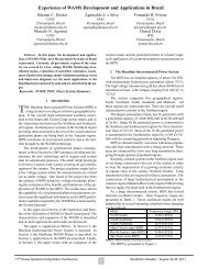
As for transient simulation, in pattern 2, 3LG fault
with 70ms duration is considered to occur at node 24.
Generator 10 is considered as a reference generator of
the system. Figures 13 and 14 show the rotor angle
difference of generators 4 and 8 and Figs. 15, 16 and 17
respectively show the output power, excitation power
and terminal voltage at the SCG node (node 4).
It can be seen from the results that system stability is
improved well by the proposed excitation control
rotor angle (rad)
1.2
1
0.8
0.6
0.4
0.2
0
-0.2
-0.4
case1
case2
case3
case4
case5
-0.6
0 2 4 6 8 10
time(s)
Figure 13: Rotor angle of generator 4
rotor angle (rad)
0.6
0.5
0.4
0.3
0.2
0.1
0
-0.1
case1
case2
case3
case4
case5
-0.2
0 2 4 6 8 10
time(s)
Figure 14: Rotor angle of generator 8
15th PSCC, Liege, 22-26 August 2005 Session 28, Paper 1, Page 6