Self-exciting point processes explain spatial-temporal patterns in crime
Self-exciting point processes explain spatial-temporal patterns in crime
Self-exciting point processes explain spatial-temporal patterns in crime

Create successful ePaper yourself
Turn your PDF publications into a flip-book with our unique Google optimized e-Paper software.
<strong>Self</strong>-<strong>excit<strong>in</strong>g</strong> <strong>po<strong>in</strong>t</strong> <strong>processes</strong> <strong>expla<strong>in</strong></strong> <strong>spatial</strong>-<strong>temporal</strong><br />
<strong>patterns</strong> <strong>in</strong> <strong>crime</strong><br />
G. O. Mohler ∗ M. B. Short † P. J. Brant<strong>in</strong>gham ‡ F. P. Schoenberg §<br />
G. E. Tita <br />
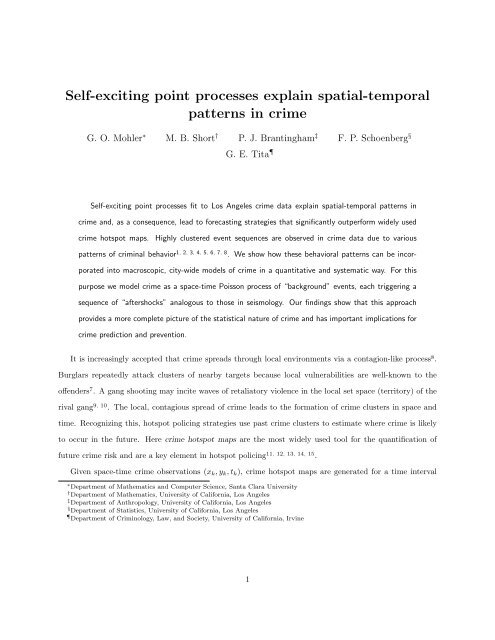
<strong>Self</strong>-<strong>excit<strong>in</strong>g</strong> <strong>po<strong>in</strong>t</strong> <strong>processes</strong> fit to Los Angeles <strong>crime</strong> data <strong>expla<strong>in</strong></strong> <strong>spatial</strong>-<strong>temporal</strong> <strong>patterns</strong> <strong>in</strong><br />
<strong>crime</strong> and, as a consequence, lead to forecast<strong>in</strong>g strategies that significantly outperform widely used<br />
<strong>crime</strong> hotspot maps. Highly clustered event sequences are observed <strong>in</strong> <strong>crime</strong> data due to various<br />
<strong>patterns</strong> of crim<strong>in</strong>al behavior 1, 2, 3, 4, 5, 6, 7, 8 . We show how these behavioral <strong>patterns</strong> can be <strong>in</strong>cor-<br />
porated <strong>in</strong>to macroscopic, city-wide models of <strong>crime</strong> <strong>in</strong> a quantitative and systematic way. For this<br />
purpose we model <strong>crime</strong> as a space-time Poisson process of “background” events, each trigger<strong>in</strong>g a<br />
sequence of “aftershocks” analogous to those <strong>in</strong> seismology. Our f<strong>in</strong>d<strong>in</strong>gs show that this approach<br />
provides a more complete picture of the statistical nature of <strong>crime</strong> and has important implications for<br />
<strong>crime</strong> prediction and prevention.<br />
It is <strong>in</strong>creas<strong>in</strong>gly accepted that <strong>crime</strong> spreads through local environments via a contagion-like process 8 .<br />
Burglars repeatedly attack clusters of nearby targets because local vulnerabilities are well-known to the<br />
offenders 7 . A gang shoot<strong>in</strong>g may <strong>in</strong>cite waves of retaliatory violence <strong>in</strong> the local set space (territory) of the<br />
rival gang 9, 10 . The local, contagious spread of <strong>crime</strong> leads to the formation of <strong>crime</strong> clusters <strong>in</strong> space and<br />
time. Recogniz<strong>in</strong>g this, hotspot polic<strong>in</strong>g strategies use past <strong>crime</strong> clusters to estimate where <strong>crime</strong> is likely<br />
to occur <strong>in</strong> the future. Here <strong>crime</strong> hotspot maps are the most widely used tool for the quantification of<br />
future <strong>crime</strong> risk and are a key element <strong>in</strong> hotspot polic<strong>in</strong>g 11, 12, 13, 14, 15 .<br />
Given space-time <strong>crime</strong> observations (xk, yk, tk), <strong>crime</strong> hotspot maps are generated for a time <strong>in</strong>terval<br />
∗ Department of Mathematics and Computer Science, Santa Clara University<br />
† Department of Mathematics, University of California, Los Angeles<br />
‡ Department of Anthropology, University of California, Los Angeles<br />
§ Department of Statistics, University of California, Los Angeles<br />
Department of Crim<strong>in</strong>ology, Law, and Society, University of California, Irv<strong>in</strong>e<br />
1
[t − T, t] by overlay<strong>in</strong>g a density plot of the function,<br />
λ(x, y, t) = <br />
t−T
function given by (1) with the function,<br />
The key differences between (1) and (2) are:<br />
λ(x, y, t) = µ(x, y) + <br />
g(x − xk, y − yk, t − tk). (2)<br />
tk
i) “Exact-repeat” <strong>crime</strong>s, multiple <strong>crime</strong>s occurr<strong>in</strong>g at the same city address, dom<strong>in</strong>ate the log-likelihood<br />
function and cause the kernel g <strong>in</strong> (2) to converge to a delta function <strong>in</strong> space. By replac<strong>in</strong>g the observations<br />
(xk, yk, tk) with (i(k), j(k), tk), where (i(k), j(k)) is the grid cell conta<strong>in</strong><strong>in</strong>g event k, this issue is resolved.<br />
ii) Forecasts are typically generated by divid<strong>in</strong>g a city map <strong>in</strong>to equally sized cells and choos<strong>in</strong>g a percentage<br />
of the cells as likely crim<strong>in</strong>al targets. Thus coarse-gra<strong>in</strong><strong>in</strong>g is useful, either before or after fitt<strong>in</strong>g the model,<br />
<strong>in</strong> order to determ<strong>in</strong>e the cells with the highest risk.<br />
In general the background <strong>in</strong>tensity µ <strong>in</strong> (2) could depend on time 20 , as the <strong>in</strong>corporation of variables such<br />
as weather and time of day could be useful, but here we assume µ is stationary. The important dist<strong>in</strong>ction<br />
between (1) and (2) is that µ is Poisson and thus does not depend on the history of the process.<br />
When the cell widths of the <strong>spatial</strong> grid are large compared to the distance over which the elevated risk<br />
spreads, <strong>in</strong> the case of burglary typically a few hundred meters 1, 11 , the coarse-gra<strong>in</strong>ed version of (2) can be<br />
approximated by the <strong>spatial</strong>ly decoupled cell <strong>in</strong>tensities,<br />
λlm(t) = µlm +<br />
<br />
{tk
of weeks or months, and for coarse-gra<strong>in</strong>ed models with cells of a few hundred meters or more we f<strong>in</strong>d that<br />
these events can be effectively modeled as background events.<br />
Whereas self-<strong>excit<strong>in</strong>g</strong> <strong>po<strong>in</strong>t</strong> process models estimate that more than 90% of burglaries and robberies <strong>in</strong><br />
the data set are background events, <strong>crime</strong> hotspot maps over-estimate the contribution of aftershocks to<br />
future <strong>crime</strong> risk by shift<strong>in</strong>g all weight to the kernel g. Furthermore, the length of the time <strong>in</strong>terval T for<br />
<strong>crime</strong> hotspot maps is typically determ<strong>in</strong>ed on the order of several weeks us<strong>in</strong>g rules of thumb, but here we<br />
estimate the decay of the excited rate to be much more rapid, on the order of several days. For other data<br />
sets, <strong>crime</strong> types, and cities, aftershocks may be more prevalent and occur over longer time scales. In such<br />
a circumstance a model of the form (1) would have greater merit. However, we argue that such a model<br />
should be determ<strong>in</strong>ed through the maximum likelihood estimation of (3) and that µ will likely play some<br />
non-trivial role.<br />
Next we <strong>in</strong>vestigate the implications of our f<strong>in</strong>d<strong>in</strong>gs for the prediction of <strong>crime</strong>. Here we compare the<br />
self-<strong>excit<strong>in</strong>g</strong> <strong>po<strong>in</strong>t</strong> process model to <strong>crime</strong> hotspot maps generated us<strong>in</strong>g a Gaussian kernel with 200m, 400m,<br />
and 800m bandwidths and 2 week, 1 month, and 2 month time <strong>in</strong>tervals. For every day k of 2005, each<br />
model assesses the risk of burglary with<strong>in</strong> each of M 2 cells partition<strong>in</strong>g an 18km by 18km region of the San<br />
Fernando Valley <strong>in</strong> Los Angeles. Based on the data from the beg<strong>in</strong>n<strong>in</strong>g of 2004 up through day k, the N<br />
cells with the highest risk (value of λ) are flagged yield<strong>in</strong>g a prediction for day k + 1. The percentage of<br />
<strong>crime</strong>s fall<strong>in</strong>g with<strong>in</strong> the flagged cells on day k + 1 is then recorded and used to measure the accuracy of<br />
each model. We then repeat this process for robbery data with<strong>in</strong> the same <strong>spatial</strong> region occurr<strong>in</strong>g dur<strong>in</strong>g<br />
the years 2006 and 2007.<br />
In Figure 3, we plot the evolv<strong>in</strong>g risk surface correspond<strong>in</strong>g to the self-<strong>excit<strong>in</strong>g</strong> <strong>po<strong>in</strong>t</strong> process forecast<strong>in</strong>g<br />
strategy outl<strong>in</strong>ed above. Each day the flagged cells change, as new <strong>crime</strong>s occur and the conditional <strong>in</strong>tensity<br />
given by (3) is updated. By accurately select<strong>in</strong>g which cells are flagged, we f<strong>in</strong>d that a large percentage of<br />
<strong>crime</strong>s can be predicted, even when flagg<strong>in</strong>g only a small percentage of cells. Directed police patrol keyed<br />
to this risk surface would maximize <strong>crime</strong> deterrence given limited resources.<br />
In Figure 4, we plot the percentage of <strong>crime</strong>s predicted averaged over the forecast<strong>in</strong>g year aga<strong>in</strong>st the<br />
percentage of flagged cells for the self-<strong>excit<strong>in</strong>g</strong> <strong>po<strong>in</strong>t</strong> process and the <strong>po<strong>in</strong>t</strong>wise maximum over all bandwidths<br />
and time <strong>in</strong>tervals for the <strong>crime</strong> hotspot maps. Depend<strong>in</strong>g on the percentage of cells flagged, the self-<strong>excit<strong>in</strong>g</strong><br />
<strong>po<strong>in</strong>t</strong> process predicts 20% to 95% more <strong>crime</strong>s on average than the <strong>crime</strong> hotspot maps. For example, with<br />
5% of the doma<strong>in</strong> flagged, the self-<strong>excit<strong>in</strong>g</strong> <strong>po<strong>in</strong>t</strong> process predicts ∼45% of robberies on average, whereas<br />
the <strong>crime</strong> hotspot maps predict ∼25%. The difference <strong>in</strong> accuracy between the two methodologies can be<br />
5
Figure 3: Evolv<strong>in</strong>g <strong>crime</strong> forecasts. (top) The conditional <strong>in</strong>tensity λ for San Fernando Valley burglary given by<br />
Equation (3) for three consecutive days <strong>in</strong> 2005. Here the cells are 500m by 500m and blue, yellow, and red correspond<br />
to progressively higher values of λ. (bottom) The 5% of cells with the highest value are flagged as the most likely<br />
burglary targets. For the second and third days, red corresponds to newly flagged cells and yellow corresponds to<br />
cells where the flag from the previous day has been removed.<br />
attributed to the <strong>crime</strong> hotspot maps failure to account for the background rate of <strong>crime</strong>. While a certa<strong>in</strong><br />
percentage of <strong>crime</strong> risk stems from near-repeat effects and evolves on a daily basis, we f<strong>in</strong>d that a large<br />
percentage is stationary and is isolated <strong>in</strong> neighborhoods with <strong>in</strong>tr<strong>in</strong>sically higher <strong>crime</strong> rates (see Figure 3).<br />
Accurate, city-wide models of <strong>crime</strong> can be constructed us<strong>in</strong>g self-<strong>excit<strong>in</strong>g</strong> <strong>po<strong>in</strong>t</strong> <strong>processes</strong>. For the 18<br />
km by 18km region of the San Fernando Valley under study, parameters of the <strong>po<strong>in</strong>t</strong> process are estimated<br />
<strong>in</strong> 1-2 m<strong>in</strong>utes and next day forecasts are generated <strong>in</strong> seconds on a laptop computer. Furthermore, self-<br />
<strong>excit<strong>in</strong>g</strong> <strong>po<strong>in</strong>t</strong> <strong>processes</strong> can be used to simulate future <strong>crime</strong> and thus daily, weekly, and monthly forecasts<br />
can be generated rapidly us<strong>in</strong>g standard <strong>po<strong>in</strong>t</strong> process simulation algorithms 18, 21 . Software based on these<br />
methods could be used by police to better focus patroll<strong>in</strong>g routes 22, 23 and by the general public to shore up<br />
the formal and <strong>in</strong>formal local community <strong>in</strong>stitutions that yield beneficial collective efficacy effects 24 .<br />
6
Figure 4: Forecast<strong>in</strong>g strategy comparison. Average daily percentage of <strong>crime</strong>s predicted plotted aga<strong>in</strong>st percentage<br />
of cells flagged for 2005 burglary (left) and 2007 robbery (right) us<strong>in</strong>g 200m by 200m cells. Here the self-<strong>excit<strong>in</strong>g</strong> <strong>po<strong>in</strong>t</strong><br />
process is compared to the <strong>po<strong>in</strong>t</strong>wise maximum over all <strong>crime</strong> hotspot maps tested. Depend<strong>in</strong>g on the percentage<br />
of cells flagged, the self-<strong>excit<strong>in</strong>g</strong> <strong>po<strong>in</strong>t</strong> process predicts 20% to 95% more <strong>crime</strong>s on average than the <strong>crime</strong> hotspot<br />
maps. For example, with only 2% of the doma<strong>in</strong> flagged the <strong>po<strong>in</strong>t</strong> process predicts 30% of the total <strong>crime</strong>s, whereas<br />
the <strong>crime</strong> hotspot maps predict less than 15%.<br />
Supplemental Information<br />
Parameter estimation<br />
Here we describe the maximum likelihood estimation of (3). For event k occurr<strong>in</strong>g <strong>in</strong> cell (l, m), the stochastic<br />
decluster<strong>in</strong>g algorithm estimates the probability pk that k is a background event as,<br />
The background <strong>in</strong>tensity is then implicitly def<strong>in</strong>ed as,<br />
µlm = (1/T ) ·<br />
pk = µlm<br />
. (4)<br />
λlm(tk)<br />
<br />
{tk
log-likelihood function can be written as,<br />
l(K0, ω) = <br />
lm<br />
<br />
− µlm +<br />
<br />
{k: i(k)=l, j(k)=m}<br />
<br />
T<br />
log λlm(tk; K0, ω) −<br />
tk<br />
<br />
g(t − tk; K0, ω)dt , (7)<br />
and is maximized us<strong>in</strong>g Monte-Carlo optimization <strong>in</strong> the search space K0 ∈ [0, 1], ω −1 ∈ (0 days, 60 days].<br />
Data<br />
The residential burglary data used <strong>in</strong> this study consists of all reported residential burglaries, collected by<br />
the Los Angeles Police Department, with<strong>in</strong> an 18km by 18km region of the San Fernando Valley dur<strong>in</strong>g the<br />
years 2004 and 2005. The robbery data used <strong>in</strong> this study consists of all reported robberies, collected by the<br />
Los Angeles Police Department, with<strong>in</strong> the same 18km by 18km region of the San Fernando Valley dur<strong>in</strong>g<br />
the years 2006 and 2007. In addition to a geocoded address, each event is associated with a reported time<br />
w<strong>in</strong>dow over which it could have occurred, often a few hour or less span. We def<strong>in</strong>ed the event time to be<br />
the mid<strong>po<strong>in</strong>t</strong> of each time w<strong>in</strong>dow. In total, the burglary data set conta<strong>in</strong>s 5,466 events and the robbery<br />
data set conta<strong>in</strong>s 2,849 events.<br />
8
References<br />
1. Johnson, S. D., Bernasco, W., Bowers, K. J., Elffers, H., Ratcliffe, J., Rengert, G., and Townsley, M. Spacetime<br />
<strong>patterns</strong> of risk: A cross national assessment of residential burglary victimization. J. Quant. Crim. 23,<br />
201–219 (2007).<br />
2. Farrell, G. and Pease, K. (Ed.) Repeat Victimization (Crim<strong>in</strong>al Justice Press, New York, 2001).<br />
3. Short, M. B., D’Orsogna, M. R., Pasour, V. B., Tita, G. E., Brant<strong>in</strong>gham, P. J., Bertozzi, A. L. and Chayes,<br />
L. A Statistical Model of Crim<strong>in</strong>al Behavior. M3AS 18, 1249–1267 (2008).<br />
4. Short, M. B., D’Orsogna, M. R., Brant<strong>in</strong>gham, P. J., and Tita, G. E. Measur<strong>in</strong>g repeat and near-repeat<br />
burglary effects, <strong>in</strong> review.<br />
5. Groff, E. Characteriz<strong>in</strong>g the Spatio-Temporal Aspects of Rout<strong>in</strong>e Activities and the Geographic Distribution<br />
of Street Robbery. Artificial Crime Analysis Systems. Liu and Eck (Eds.) IGI Global: Hershey, PA (2008).<br />
6. Bernasco, W. and Luykx, F. Effects of attractiveness, opportunity and accessiblity to burglars on residential<br />
burglary rates of urban neighborhoods. Crim<strong>in</strong>ology 41, 981–1001 (2003).<br />
7. Bernasco, W. and Nieuwbeerta, P. How do residential burglars select targe areas? A new approach to the<br />
analysis of crim<strong>in</strong>al location choice. Brit. J. Crim<strong>in</strong>ology 45, 296–315 (2005).<br />
8. Johnson, S. Repeat burglary victimisation: a tale of two theories. Journal of Experimental Crim<strong>in</strong>ology 4,<br />
215–240 (2008).<br />
9. Tita, G. and Ridgeway, G. The Impact of Gang Formation on Local Patterns of Crime. Journal of Research<br />
on Crime and Del<strong>in</strong>quency 44 (2), 208–237 (2007).<br />
10. Cohen, J. and Tita, G. Spatial Diffusion <strong>in</strong> Homicide: Explor<strong>in</strong>g a General Method of Detect<strong>in</strong>g Spatial<br />
Diffusion Processes. Journal of Quantitative Crim<strong>in</strong>ology 15 (4), 451–493 (1999).<br />
11. Bowers, K. J., Johnson, S. D., and Pease, K. Prospective Hot-Spott<strong>in</strong>g: The Future of Crime Mapp<strong>in</strong>g?<br />
Brit. J. Crim<strong>in</strong>ol. 44, 641–658 (2004).<br />
12. Cha<strong>in</strong>ey, S. and Ratcliffe, J. GIS and Crime Mapp<strong>in</strong>g (Wiley, West Sussex, 2005).<br />
13. Cha<strong>in</strong>ey, S., Tompson, L., and Uhlig S. The Utility of Hotspot Mapp<strong>in</strong>g for Predict<strong>in</strong>g Spatial Patterns of<br />
Crime. Security Journal 21, 4–28 (2008).<br />
14. Braga, A. Hot Spots Polic<strong>in</strong>g and Crime Prevention: A Systematic Review of Randomized Controlled Trials.<br />
Journal of Experimental Crim<strong>in</strong>ology, 1 3, 317–342 (2005).<br />
15. Caeti, T. Houstons Targeted Beat Program: A Quasi-Experimental Test of Police Patrol Strategies.<br />
Ph.D. dissertation, Sam Houston State University. Ann Arbor, Michgan: University Microfilms International<br />
(1999).<br />
16. Gardner, J. K. and Knopoff, L. Is the sequence of earthquakes <strong>in</strong> Southern California, with aftershocks<br />
removed, Poissonian? Bullet<strong>in</strong> of the Seismological Society of America 64 (5), 1363–1367 (1974).<br />
17. Ogata, Y. Spate-time <strong>po<strong>in</strong>t</strong> process models for earthquake occurrences, Ann. Inst. Statist. Math. 50 (2),<br />
379–402 (1998).<br />
18. Daley, D. and Vere-Jones, D. An Introduction to the Theory of Po<strong>in</strong>t Processes (Spr<strong>in</strong>ger, New York,<br />
2003).<br />
9
19. Zhuang, J., Ogata, Y., and Vere-Jones, D. Stochastic Decluster<strong>in</strong>g of Space-Time Earthquake Occurences.<br />
JASA 97 (458), 369–380 (2002).<br />
20. Schoenberg, F.P., Chang, C., Keeley, J., Pompa, J., Woods, J., and Xu, H. A Critical Assessment of the<br />
Burn<strong>in</strong>g Index <strong>in</strong> Los Angeles County, California. Int. J. Wildland Fire 16 (4), 473–483 (2007).<br />
21. Ogata, Y. On Lewis’ Simulation Method for Po<strong>in</strong>t Processes. IEEE 27 (1), 23–31 (1981).<br />
22. Sherman, L. and Weisburd, D. General Deterrent Effects of Police Patrol <strong>in</strong> Crime Hot Spots: A Randomized<br />
Controlled Trial. Justice Quarterly 12, 625–648 (1995).<br />
23. Weisburd, D. and Eck, J. E. What Can Police Do to Reduce Crime, Disorder, and Fear? The ANNALS of<br />
the American Academy of Political and Social Science 593, 42–65 (2004).<br />
24. Sampson, R. J., Raudenbush, S. W., and Earls, F. Neighborhoods and Violent Crime: A Multilevel Study of<br />
Collective Efficacy. Science 277, 918–924 (1997).<br />
Acknowledgements<br />
The authors would like to thank the National Science Foundation for support through grant BCS-0527388.<br />
Correspondence and Requests for materials should be addressed to:<br />
George Mohler<br />
Santa Clara University<br />
Department of Mathematics and Computer Science<br />
Santa Clara, CA<br />
gmohler@scu.edu<br />
10