Propensity Scores: Helping Non-Statisticians Get The Message
Propensity Scores: Helping Non-Statisticians Get The Message
Propensity Scores: Helping Non-Statisticians Get The Message

Create successful ePaper yourself
Turn your PDF publications into a flip-book with our unique Google optimized e-Paper software.
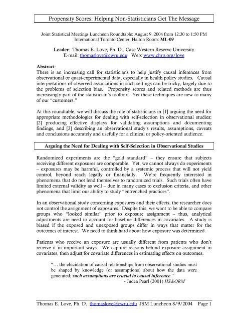
<strong>Propensity</strong> <strong>Scores</strong>: <strong>Helping</strong> <strong>Non</strong>-<strong>Statisticians</strong> <strong>Get</strong> <strong>The</strong> <strong>Message</strong><br />
Joint Statistical Meetings Luncheon Roundtable: August 9, 2004 from 12:30 to 1:50 PM<br />
International Toronto Center, Halton Room: ML-09<br />
Leader: Thomas E. Love, Ph. D., Case Western Reserve University<br />
E-mail: thomaslove@cwru.edu Web: www.chrp.org/love<br />
Abstract:<br />
<strong>The</strong>re is an increasing call for statisticians to help justify causal inferences from<br />
observational or quasi-experimental data, especially in health policy studies. Causal<br />
interpretations of observed associations in such settings can be tricky, largely due to<br />
the problems of selection bias. <strong>Propensity</strong> scores and related methods are thus<br />
increasingly part of the statistician’s toolbox. Yet these techniques are new to many<br />
of our “customers.”<br />
At this roundtable, we will discuss the role of statisticians in [1] arguing the need for<br />
appropriate methodologies for dealing with self-selection in observational studies;<br />
[2] producing effective displays for validating assumptions and documenting<br />
findings, and [3] describing an observational study’s results, assumptions, caveats<br />
and conclusions accurately and usefully for a clinical or policy-oriented audience.<br />
Arguing the Need for Dealing with Self-Selection in Observational Studies<br />
Randomized experiments are the “gold standard” – they ensure that subjects<br />
receiving different exposures are comparable. Yet, we cannot always do experiments<br />
– exposures may be harmful, controlled by a systemic process that will not yield<br />
control, beyond reach legally or financially. We’re frequently interested in<br />
phenomena that do not lend themselves to randomized trials. Such trials often have<br />
limited external validity as well – due in many cases to exclusion criteria, and other<br />
phenomena that limit our ability to study “entrenched practices”.<br />
In an observational study concerning exposures and their effects, the researcher does<br />
not control the assignment of exposures. Despite this, we want to be able to compare<br />
groups who “looked similar” prior to exposure assignment – thus, analytical<br />
adjustments are need to account for baseline differences in covariates. A study is<br />
biased if the exposed and unexposed groups differ in ways that matter for the<br />
outcomes of interest. We need to think hard about how exposure was determined.<br />
Patients who receive an exposure are usually different from patients who don’t<br />
receive it in important ways. We capture reasons behind exposure assignment in<br />
covariates, then adjust for covariate differences in estimating effects on outcomes.<br />
“… the elucidation of causal relationships from observational studies must<br />
be shaped by knowledge (or assumptions) about how the data were<br />
generated; such assumptions are crucial to causal inference.”<br />
- Judea Pearl (2001) HS&ORM<br />
Thomas E. Love, Ph. D. thomaslove@cwru.edu JSM Luncheon 8/9/2004 Page 1
<strong>Propensity</strong> <strong>Scores</strong>: <strong>Helping</strong> <strong>Non</strong>-<strong>Statisticians</strong> <strong>Get</strong> <strong>The</strong> <strong>Message</strong><br />
Seven Key Aspects of Research Architecture: Judgments About Causation<br />
(Feinstein Model for the evaluation of the scientific quality of cause-effect research,<br />
as modified by Neal V. Dawson, MD nvd@cwru.edu)<br />
Goal: Comparability of the Groups Who Did and Did Not Receive the<br />
Exposure of Interest (Except for the Actual Receipt of Exposure)<br />
Selection Performance<br />
Detection<br />
Assembly Susceptibility<br />
Co-Intervention<br />
Sample<br />
Population<br />
[R or S1]<br />
Group A<br />
Group B<br />
Exposure A<br />
Exposure B<br />
Co-I C<br />
[S2]<br />
Co-I C<br />
Outcome A<br />
Outcome B<br />
Transfer<br />
Collected<br />
Groups<br />
1. Distorted Assembly: <strong>The</strong> sample should reflect the population to which results<br />
will be generalized. Application of specific inclusion/exclusion criteria will<br />
determine the pool of baseline characteristics of the sample.<br />
2. Selection Bias: Bias can occur when subjects are selected to receive an exposure<br />
or co-intervention – especially when exposure is based on baseline covariates,<br />
and covariates are related to different likelihoods of outcome. Unmeasured<br />
covariates may or may not also be associated with measured characteristics.<br />
3. Susceptibility Bias / Case Mix / Severity: Comparability of baseline<br />
characteristics of the exposure groups – are there importantly different<br />
expectations at baseline of the outcome of interest.<br />
4. Performance Bias: How “well” do patients receive exposures (i.e. differences in<br />
dosage schedules, compliance rates, etc.)<br />
5. Co-Interventions (Another Opportunity for Selection): Additional (medical)<br />
interventions beyond the exposure of interest that may influence the likelihood of<br />
achieving the outcome.<br />
6. Outcome Bias: Process for determining the status of the outcome of interest in<br />
each group is applied unequally – differences in surveillance, diagnostic<br />
interpretation or testing, etc.<br />
7. Transfer Bias: Members of the original or complete cohorts of A and B may be<br />
lost to dropout, intra-study exclusions, crossover, during statistical<br />
manipulations, etc.<br />
“Care in design and implementation will be rewarded with useful and clear<br />
study conclusions… Elaborate analytical methods will not salvage poor<br />
design or implementation of a study.”<br />
- National Academy of Sciences Report (Meyer and Feinberg 1992, p. 106)<br />
Thomas E. Love, Ph. D. thomaslove@cwru.edu JSM Luncheon 8/9/2004 Page 2
<strong>Propensity</strong> <strong>Scores</strong>: <strong>Helping</strong> <strong>Non</strong>-<strong>Statisticians</strong> <strong>Get</strong> <strong>The</strong> <strong>Message</strong><br />
<strong>The</strong> standard ANCOVA procedure for mitigating selection bias: (Risk Adjustment)<br />
1. Capture as many important variables as possible and include them in the<br />
model, along with an indicator IT or whether or not the subject received the<br />
treatment.<br />
2. Identify the coefficient of the IT indicator as a measure of the risk-adjusted<br />
“association” between receipt of treatment and the outcome.<br />
3. Discuss and evaluate alternative explanations for the observed association<br />
other than “causality”.<br />
<strong>The</strong>re is a clear need to …<br />
“move beyond these informal techniques (that often perform well in the<br />
hands of ‘master users’) to established conceptual frameworks and “userfriendly”<br />
protocols.”<br />
–Ash, Normand, Duan (2001) HS&ORM<br />
Validating Assumptions: <strong>The</strong> Issue of Overlap<br />
How Much Overlap In <strong>The</strong> Covariates<br />
Do We Want?<br />
Covariate of<br />
Interest<br />
1<br />
0<br />
Not Treated Treated<br />
• If those who receive<br />
treatment don’t overlap (in<br />
terms of covariates) with<br />
those who receive the control,<br />
we’ve got nothing to<br />
compare.<br />
• Modeling, no matter how<br />
sophisticated, can’t help us to<br />
develop information out of<br />
thin air.<br />
What if Treated and Untreated<br />
Groups Don’t Overlap Completely?<br />
<strong>Propensity</strong> Score<br />
1<br />
0<br />
Not Treated Treated<br />
• Inferences for the causal<br />
effects of treatment on the<br />
subjects with no overlap<br />
cannot be drawn without<br />
heroic modeling<br />
assumptions.<br />
• Usually, we’d exclude<br />
these treated subjects, and<br />
explain separately.<br />
What if Treated and Untreated<br />
Groups Overlap, but minimally?<br />
Covariate of<br />
Interest<br />
1<br />
0<br />
Not Treated Treated<br />
•No help.<br />
• <strong>The</strong> information available<br />
to infer treatment effect<br />
will reside almost entirely<br />
in the few patients who<br />
overlap.<br />
• Need to think hard about<br />
whether useful inferences<br />
will be possible.<br />
How Much Overlap In <strong>The</strong> <strong>Propensity</strong><br />
<strong>Scores</strong> Do We Want?<br />
<strong>Propensity</strong> to<br />
receive treatment<br />
1<br />
0<br />
Not Treated Treated<br />
<strong>Propensity</strong> to<br />
receive treatment<br />
1<br />
0<br />
Not Treated Treated<br />
<strong>Propensity</strong> to<br />
receive treatment<br />
1<br />
0<br />
Not Treated Treated<br />
Thomas E. Love, Ph. D. thomaslove@cwru.edu JSM Luncheon 8/9/2004 Page 3
<strong>Propensity</strong> <strong>Scores</strong>: <strong>Helping</strong> <strong>Non</strong>-<strong>Statisticians</strong> <strong>Get</strong> <strong>The</strong> <strong>Message</strong><br />
Aspirin Use and Mortality Example from Gum et al. (2001) JAMA<br />
Aspirin Use and Mortality<br />
• 6174 consecutive adults undergoing stress<br />
echocardiography for evaluation of known or<br />
suspected coronary disease.<br />
• 2310 (37%) were taking aspirin (treatment).<br />
• Main Outcome: all-cause mortality<br />
• Median follow-up: 3.1 years<br />
• Univariate Analysis: 4.5% of aspirin patients<br />
died, and 4.5% of non-aspirin patients died…<br />
• Unadjusted Hazard Ratio: 1.08 (0.85, 1.39)<br />
Gum PA et al. (2001) JAMA, 1187-1194.<br />
Baseline Characteristics According to<br />
Aspirin Use (before matching)<br />
Variable<br />
Age, years<br />
Body mass index, kg/m 2<br />
Ejection fraction, %<br />
Resting heart rate, beats/min<br />
Resting systolic BP, mm Hg<br />
Resting diastolic BP, mm Hg<br />
Heart rate recovery, beats/min<br />
Peak exercise cap., men (METs)<br />
Aspirin*<br />
(n = 2310)<br />
62 (11)<br />
29 (5)<br />
50 (9)<br />
74 (13)<br />
141 (21)<br />
85 (11)<br />
28 (11)<br />
8.6 (2.4)<br />
No Aspirin*<br />
(n = 3864)<br />
56 (12)<br />
30 (7)<br />
53 (7)<br />
79 (14)<br />
138 (20)<br />
86 (11)<br />
30 (12)<br />
9.1 (2.6)<br />
Peak exercise capacity, women 6.6 (2.0) 7.3 (2.1)<br />
*Cells contain mean (SD)<br />
P value<br />
< .001<br />
< .001<br />
< .001<br />
< .001<br />
< .001<br />
.04<br />
< .001<br />
< .001<br />
< .001<br />
Baseline Characteristics According to<br />
Aspirin Use (after matching)<br />
Variable<br />
Age, years<br />
Body mass index, kg/m 2<br />
Ejection fraction, %<br />
Resting heart rate, beats/min<br />
Resting systolic BP, mm Hg<br />
Resting diastolic BP, mm Hg<br />
Heart rate recovery, beats/min<br />
Peak exercise cap., men (METs)<br />
Aspirin*<br />
(n = 1351)<br />
60 (11)<br />
29 (6)<br />
51 (8)<br />
77 (13)<br />
141 (21)<br />
85 (11)<br />
28 (12)<br />
8.7 (2.5)<br />
No Aspirin*<br />
(n = 1351)<br />
61 (11)<br />
29 (6)<br />
51 (9)<br />
76 (14)<br />
141 (21)<br />
86 (11)<br />
28 (11)<br />
8.3 (2.5)<br />
Peak exercise capacity, women 6.5 (2.0) 6.7 (2.0)<br />
*Cells contain mean (SD)<br />
P value<br />
.16<br />
.83<br />
.65<br />
.13<br />
.68<br />
.57<br />
.82<br />
.01<br />
.13<br />
What Would Be Relevant Covariates<br />
for Adjustment?<br />
•Demographics (Age, Sex)<br />
• Cardiovascular risk factors<br />
• Coronary disease history<br />
• Use of other medications<br />
• Ejection fraction<br />
• Exercise capacity<br />
• Heart rate recovery<br />
• Echocardiographic ischemia<br />
Variable<br />
Men<br />
Result of adjusting<br />
for these factors:<br />
Aspirin use now<br />
associated with<br />
reduced mortality:<br />
Hazard Ratio: 0.67<br />
95% CI: (.51, .87)<br />
p = .002<br />
Baseline Characteristics By Aspirin<br />
Use (in %) (before matching)<br />
Clinical history: diabetes<br />
hypertension<br />
prior coronary artery disease<br />
congestive heart failure<br />
Medication use: Beta-blocker<br />
Aspirin<br />
(n = 2310)<br />
77.0<br />
16.8<br />
53.0<br />
69.7<br />
20.1<br />
< .001<br />
ACE inhibitor<br />
13.0 11.4 < .001<br />
• Baseline characteristics appear very dissimilar: 25 of 31<br />
covariates have p < .001, 28 of 31 have p < .05.<br />
• Aspirin user covariates indicate higher mortality risk.<br />
Variable<br />
Men<br />
5.5<br />
35.1<br />
No Aspirin<br />
(n = 3864)<br />
56.1<br />
11.2<br />
40.6<br />
4.6<br />
14.2<br />
Baseline Characteristics By Aspirin<br />
Use [%] (after matching)<br />
Clinical history: diabetes<br />
hypertension<br />
prior coronary artery disease<br />
congestive heart failure<br />
Medication use: Beta-blocker<br />
ACE inhibitor<br />
Aspirin<br />
(n = 1351)<br />
70.4<br />
15.0<br />
50.3<br />
48.3<br />
48.8<br />
P value<br />
< .001<br />
< .001<br />
< .001<br />
.12<br />
< .001<br />
• Baseline characteristics similar in matched users and non-users.<br />
• 30 of 31 covariates show NS difference between matched users<br />
and non-users. [Peak exercise capacity for men is p = .01]<br />
5.8<br />
26.1<br />
15.5<br />
No Aspirin<br />
(n = 1351)<br />
72.1<br />
15.3<br />
51.7<br />
6.6<br />
26.5<br />
15.8<br />
P value<br />
Thomas E. Love, Ph. D. thomaslove@cwru.edu JSM Luncheon 8/9/2004 Page 4<br />
.33<br />
.83<br />
.46<br />
.79<br />
.43<br />
.79<br />
.79
<strong>Propensity</strong> <strong>Scores</strong>: <strong>Helping</strong> <strong>Non</strong>-<strong>Statisticians</strong> <strong>Get</strong> <strong>The</strong> <strong>Message</strong><br />
Multivariate and <strong>Propensity</strong> Score Matching Algorithm in R: See<br />
http://jsekhon.fas.harvard.edu/matching/<br />
Displays for Validating Assumptions: Covariate Balance After Adjustment<br />
1<br />
0.9<br />
0.8<br />
0.7<br />
0.6<br />
0.5<br />
0.4<br />
0.3<br />
0.2<br />
0.1<br />
0<br />
Are <strong>The</strong> Covariates Balanced?<br />
“P values Plot”<br />
31 covariates provided in paper’s Tables.<br />
Aspirin <strong>Propensity</strong> Score M atching: Do Covariates Balance?<br />
Unmatched P value Matched P value<br />
PeakExMen<br />
RestHrtRate<br />
PeakExWom<br />
Age<br />
PriorPCInterv<br />
Nifedipine<br />
StressIsche<br />
%Men<br />
PriorCABG<br />
CongestHF<br />
Hypertension<br />
EchoLV<br />
PriorQMI<br />
RDiasBP<br />
Fitness<br />
LipidLow<br />
Ischemic<br />
AtrialFib<br />
EjectionFrac<br />
RSysBP<br />
ChestPain<br />
PriorCAD<br />
BetaBl<br />
ACEinh<br />
HRRecov<br />
Diabetes<br />
BMI<br />
MayoRisk<br />
Digoxin<br />
Tobacco<br />
Diltiazem<br />
Covariate Balance for Aspirin Study<br />
PriorCAD<br />
PriorPCInterv<br />
PriorCABG<br />
LipidLow<br />
MayoRisk<br />
Age<br />
BetaBl<br />
%Men<br />
StressIsche<br />
EchoLV<br />
PriorQMI<br />
Diltiazem<br />
Hypertension<br />
Ischemic<br />
Diabetes<br />
RSysBP<br />
Nifedipine<br />
ACEinh<br />
Digoxin<br />
CongestHF<br />
ChestPain<br />
AtrialFib<br />
Fitness<br />
Tobacco<br />
RDiasBP<br />
BMI<br />
HRRecov<br />
PeakExMen<br />
PeakExWom<br />
RestHrtRate<br />
EjectionFrac<br />
Before Match<br />
After Match<br />
-50 0 50 100<br />
Asp - No Asp Standardized Difference (%)<br />
Absolute Value of Standardized Difference, %<br />
140<br />
120<br />
100<br />
Absolute Standardized Differences<br />
PriorCAD<br />
PriorPCInterv<br />
PriorCABG<br />
LipidLow<br />
MayoRisk<br />
Age<br />
BetaBl<br />
%Men<br />
EjectionFrac<br />
RestHrtRate<br />
PeakExWom<br />
StressIsche<br />
EchoLV<br />
PriorQMI<br />
Diltiazem<br />
Hypertension<br />
PeakExMen<br />
Ischemic<br />
HRRecov<br />
BMI<br />
Diabetes<br />
RSysBP<br />
Nifedipine<br />
ACEinh<br />
RDiasBP<br />
Tobacco<br />
Digoxin<br />
CongestHF<br />
Fitness<br />
ChestPain<br />
AtrialFib<br />
Covariate Balance for Aspirin Study<br />
80<br />
60<br />
40<br />
20<br />
0<br />
Unmatched Matched<br />
Prior CAD<br />
PriorPCInterv<br />
Prior CABG<br />
LipidLowDrug<br />
MayoRisk>1<br />
Age<br />
BetaBlocker<br />
%M en<br />
EjectionFrac<br />
RestHrtRate<br />
PeakExWom<br />
StressIsche<br />
EchoLV<br />
PriorQMI<br />
Diltiazem<br />
Hypertension<br />
PeakExMen<br />
Ischemic<br />
HRRecov<br />
BM I<br />
Diabetes<br />
RestSysBP<br />
Nifedipine<br />
ACEinhibitor<br />
RestDiasBP<br />
Tobacco<br />
Digoxin<br />
CongestiveHF<br />
FitnessP/F<br />
ChestPain<br />
AtrialFibrilat<br />
Absolute Value of Standardized Difference<br />
plotted for 31 covariates (in Excel).<br />
Before Match<br />
After Match<br />
0 20 40 60 80 100 120<br />
Asp - NoAsp Absolute Standardized Difference (%)<br />
Thomas E. Love, Ph. D. thomaslove@cwru.edu JSM Luncheon 8/9/2004 Page 5
<strong>Propensity</strong> <strong>Scores</strong>: <strong>Helping</strong> <strong>Non</strong>-<strong>Statisticians</strong> <strong>Get</strong> <strong>The</strong> <strong>Message</strong><br />
Who’s <strong>Get</strong>ting Matched Here?<br />
Where Do <strong>The</strong> <strong>Propensity</strong> <strong>Scores</strong> Overlap?<br />
<strong>Propensity</strong> to<br />
Use Aspirin<br />
1<br />
0<br />
<strong>Non</strong>-users Users<br />
Caveat: This simulation depicts<br />
what often happens.<br />
Aspirin users we won’t be<br />
able to match effectively<br />
Aspirin users for whom<br />
we might realistically<br />
find a good match in our<br />
pool of non-users<br />
Which Aspirin Users <strong>Get</strong> Matched?<br />
• 652 of the 1351 matched aspirin users had had prior<br />
coronary artery disease (48.3%).<br />
• 957 of the 959 unmatched aspirin users had had prior<br />
coronary artery disease (99.8%).<br />
Variable % of Matched % of Unmatched Stdzd Diff<br />
Prior CAD 48.3<br />
99.8 -145<br />
Prior PCI 12.3<br />
52.2<br />
-95<br />
Lipid-low th 20.8<br />
51.5<br />
-68<br />
Prior CABG 18.6<br />
45.7<br />
-61<br />
β-blocker 26.1<br />
47.9<br />
-46<br />
Tobacco 11.9<br />
7.3<br />
+16<br />
Describing the Results of an Observational Study Accurately and Usefully<br />
Rosenbaum’s Four Specific Suggestions (2002 book, p. 368)<br />
• Design Observational Studies<br />
o Exert as much experimental control as possible, carefully consider the selection process,<br />
and anticipate hidden biases.<br />
• Focus on Simple Comparisons<br />
o Increase impact of results on consumers<br />
• Compare Subjects Who Looked Comparable Prior to Treatment<br />
• Use Sensitivity Analyses to Inform Discussions of Hidden Bias Due to<br />
Unobserved Covariates<br />
o Sensitivity analysis asks how much hidden bias would need to be present to explain the<br />
differing outcomes in the exposed and control groups.<br />
What Should Always Be Done in an Observational Study and Often Isn’t<br />
• Collect data so as to be able to model selection<br />
• Demonstrate selection bias<br />
• Ensure covariate overlap for comparability<br />
• Evaluate covariate balance after adjustment<br />
• Specify relevant post-adjustment population with care<br />
• Model or estimate treatment effect in light of selection bias adjustments<br />
• Estimate sensitivity of results to potential hidden biases<br />
Instrumental Variables vs. <strong>Propensity</strong> Methods vs. “Standard Risk Adjustment”<br />
IV analysis has a long history in economics, where we are often facing “weak” data.<br />
<strong>The</strong> methods are attractive because they mirror RCT – instrument should adjust for<br />
both overt and hidden biases, and the resulting local average treatment effect<br />
estimates are sometimes more interesting than estimates from propensity models. It<br />
remains awfully difficult to justify the IV assumptions, although some specific<br />
examples (noncompliance in randomized trials) look well-suited to instruments.<br />
Thomas E. Love, Ph. D. thomaslove@cwru.edu JSM Luncheon 8/9/2004 Page 6
<strong>Propensity</strong> <strong>Scores</strong>: <strong>Helping</strong> <strong>Non</strong>-<strong>Statisticians</strong> <strong>Get</strong> <strong>The</strong> <strong>Message</strong><br />
A Partial Bibliography<br />
Articles I Have Used in A Short Course on <strong>Propensity</strong> Methods<br />
1. Connors AF, Speroff T, Dawson NV, Thomas C, et al. (1996) <strong>The</strong><br />
effectiveness of right heart catheterization in the initial care of critically ill<br />
patients (with Editorial). Journal of the American Medical Association, 276: 889-897,<br />
915-918. [<strong>Propensity</strong> scores in action: matching and multivariate adjustment.]<br />
2. D'Agostino RB Jr. (1998) <strong>Propensity</strong> score methods for bias reduction in the<br />
comparison of a treatment to a non-randomized control group. Statistics in<br />
Medicine, 17: 2265-2281. [Readable introduction to matching, stratification and<br />
regression with propensity scores.]<br />
3. Earle CC, Tsai JS, et al. (2001) Effectiveness of chemotherapy for advanced<br />
lung cancer in the elderly: Instrumental variable and propensity analysis. Journal<br />
of Clinical Oncology, 19: 1064-1070. [Interesting combination of instrumental<br />
variables and propensity analyses.]<br />
4. Gum PA, Thamilarasan M, Watanabe J, et al. (2001) Aspirin use and allcause<br />
mortality among patients being evaluated for known or suspected coronary<br />
artery disease. Journal of the American Medical Association, 286(10)[Sep 12]: 1187-<br />
1194. Editorial: Radford MJ and Foody JM, pp. 1228-1230. [PS matching with<br />
nonproportional hazards models for survival analysis, the results show interesting<br />
impact of bias adjustment – editorial motivates observational studies vs. RCTs<br />
discussion, discusses cluster analysis and hierarchical modeling.]<br />
5. Hullsiek KH and Louis TA (2002) <strong>Propensity</strong> score modeling strategies for<br />
the causal analysis of observational data. Biostatistics, 3, 179-193.<br />
6. Joffe MM and Rosenbaum PR (1999) <strong>Propensity</strong> scores. American Journal of<br />
Epidemiology, 150: 327-333. [Motivation for propensity score approaches, as well<br />
as a set of extensions – to case/control studies and to dose-response issues.]<br />
7. Normand SLT, Landrum MB, Guadagnoli E, Ayanian JZ et al. (2001)<br />
Validating recommendations for coronary angiography following acute<br />
myocardial infarction in the elderly: A matched analysis using propensity scores.<br />
Journal of Clinical Epidemiology, 54: 387-398. [PS matching with calipers.<br />
Interesting discussion of covariate balance, leads to odds ratios, assessment of<br />
association through Mantel-Haenszel, survival rates, etc.]<br />
8. Rosenbaum PR (1991) Discussing hidden bias in observational studies. Annals<br />
of Internal Medicine, 115: 901-905. [Introduction to sensitivity analysis, related<br />
issues.]<br />
9. Rosenbaum PR and Rubin DB (1984) Reducing bias in observational studies<br />
using subclassification on the propensity score, Journal of the American Statistical<br />
Association, 79: 516-524. [One of the seminal papers – presents subclassification on<br />
the propensity score.]<br />
10. Rubin DB (1997) Estimating causal effects from large data sets using<br />
propensity scores. Annals of Internal Medicine, 127: 757-763. [Introductory<br />
discussion, very readable.]<br />
Thomas E. Love, Ph. D. thomaslove@cwru.edu JSM Luncheon 8/9/2004 Page 7
<strong>Propensity</strong> <strong>Scores</strong>: <strong>Helping</strong> <strong>Non</strong>-<strong>Statisticians</strong> <strong>Get</strong> <strong>The</strong> <strong>Message</strong><br />
Relevant Books on Related Issues<br />
11. Rosenbaum PR (2002) Observational Studies, 2 nd Edition. Springer.<br />
12. Cochran WG (1983) Planning and Analysis of Observational Studies Wiley.<br />
13. Cook TD and Campbell DC (1979) Quasi-Experimentation Chicago: Rand<br />
McNally.<br />
14. Elwood JM (1988) Causal Relationships in Medicine New York: Oxford Univ<br />
Press.<br />
15. Pearl J (2000) Causality: Models, Reasoning, Inference New York: Cambridge<br />
Univ Press.<br />
16. Shadish WR, Cook TD and Campbell DT (2002) Experimental and Quasi-<br />
Experimental Designs for Generalized Causal Inference Boston: Houghlin-Mifflin.<br />
<strong>Propensity</strong> Score Methodology – Development and Extensions<br />
17. D'Agostino RB Jr and Rubin DB (2000) Estimating and using propensity<br />
scores with partially missing data. Journal of the American Statistical Association<br />
[JASA] 95, 749-759<br />
18. Drake C and Fisher L (1995) Prognostic models and the propensity score.<br />
International Journal of Epidemiology 24: 183-187<br />
19. Leon AC, Mueller TI et al. (2001) A dynamic adaptation of the propensity<br />
score adjustment for effectiveness analysis of ordinal doses of treatment. Statistics<br />
in Medicine 20: 1487-1498<br />
20. Lu B, Zanutto E, Hornik R and Rosenbaum PR (2002) Matching with doses<br />
in an observational study of a media campaign against drug abuse. JASA 96,<br />
1245-1253.<br />
21. Rosenbaum PR and Rubin DB (1983) <strong>The</strong> central role of the propensity score<br />
in observational studies for causal effects. Biometrika 70, 41-55<br />
22. Rosenbaum PR (1984) <strong>The</strong> consequences of adjustment for a concomitant<br />
variable that has been affected by the treatment, Journal of the Royal Statistical<br />
Society, Ser. A 147, 656-666.<br />
23. Rosenbaum PR and Rubin DB (1985) Constructing a control group using<br />
multivariate matched sampling methods that incorporate the propensity score.<br />
<strong>The</strong> American Statistician 39, 33-38.<br />
24. Rosenbaum PR (1987) Model-based direct adjustment. JASA 82, 387-394.<br />
25. Rubin DB and Thomas N (1996) Matching using estimated propensity scores:<br />
Relating theory to practice. Biometrics 52: 249-264.<br />
26. Rubin DB and Thomas N (2000) Combining propensity score matching with<br />
additional adjustments for prognostic covariates. JASA 95, 573-585.<br />
27. Wang J, Donnan PT et al. (2001) <strong>The</strong> multiple propensity score for analysis<br />
of dose-response relationships in drug safety studies, Pharmacoepidemiology and<br />
Drug Safety 10, 105-111.<br />
Instrumental Variables and Related Ideas<br />
Thomas E. Love, Ph. D. thomaslove@cwru.edu JSM Luncheon 8/9/2004 Page 8
<strong>Propensity</strong> <strong>Scores</strong>: <strong>Helping</strong> <strong>Non</strong>-<strong>Statisticians</strong> <strong>Get</strong> <strong>The</strong> <strong>Message</strong><br />
28. Angrist JD, Imbens GW and Rubin DB (1996) Identification of causal effects<br />
using instrumental variables (with Comments). JASA 91, 444-472. [Key IV paper<br />
for statisticians.]<br />
29. Greenland S (2000) An introduction to instrumental variables for<br />
epidemiologists, International Journal of Epidemiology 29, 722-729.<br />
30. Lavori PW, Dawson R, Mueller TB (1994) Causal estimation of time-varying<br />
treatment effects in observational studies - Application to depressive disorder,<br />
Statistics in Medicine 13, 1089-1100.<br />
31. McClellan M, McNeil BJ, Newhouse JP (1994) Does more intensive<br />
treatment of acute myocardial infarction in the elderly reduce mortality?<br />
Analysis using instrumental variables, Journal of the American Medical Association<br />
272, 859-866.<br />
32. Newhouse JP, McClellan M (1998) Econometrics in outcomes research: the<br />
use of instrumental variables, Annual Review of Public Health 19, 17-34.<br />
Sensitivity Analysis<br />
33. Greenland S (1996) Basic methods for sensitivity analysis of biases,<br />
International Journal of Epidemiology, 25, 1107-1116.<br />
34. Lin DY, Psaty BM and Kronmal RA (1998) Assessing the sensitivity of<br />
regression results to unmeasured confounders in observational studies, Biometrics,<br />
54, 948-963.<br />
35. Rosenbaum PR (1999) Choice as an Alternative to Control in Observational<br />
Studies (with Comments), Statistical Science, 14, 259-304.<br />
36. Rosenbaum PR and Rubin DB (1983) Assessing sensitivity to an unobserved<br />
binary covariate in an observational study with binary outcome, Journal of the<br />
Royal Statistical Society, Series B, 45, 212-218.<br />
Other Interesting Papers<br />
37. Abel U, Koch A (1999) <strong>The</strong> role of randomization in clinical studies: Myths<br />
and beliefs, Journal of Clinical Epidemiology 52, 487-497.<br />
38. Cepeda MS, Boston R et al. (2003) Comparison of logistic regression versus<br />
propensity score when the number of events are low and there are multiple<br />
confounders, Am J Epidemiology, 158, 280-287.<br />
39. Cochran WG (1968) <strong>The</strong> effectiveness of adjustment by subclassification in<br />
removing bias in observational studies, Biometrics 24, 295-313.<br />
40. Copas JB and Li HG (1997) Inference for <strong>Non</strong>-Random Samples (with<br />
discussion), Journal of the Royal Statistical Society, Series B 59, 55-95.<br />
41. Greenland S and Morgenstern H (2001) Confounding in health research,<br />
Annual Review of Public Health 22, 189-212.<br />
42. Greenland S (2000) Causal analysis in the health sciences, JASA 95, 286-289.<br />
43. Kraemer HC, Stice E et al. (2001) How do risk factors work together?<br />
Mediators, moderators and independent, overlapping, and proxy risk factors,<br />
American Journal of Psychiatry 158, 848-856.<br />
Thomas E. Love, Ph. D. thomaslove@cwru.edu JSM Luncheon 8/9/2004 Page 9
<strong>Propensity</strong> <strong>Scores</strong>: <strong>Helping</strong> <strong>Non</strong>-<strong>Statisticians</strong> <strong>Get</strong> <strong>The</strong> <strong>Message</strong><br />
44. Little RJA and Rubin DB (2000) Causal effects in clinical and<br />
epidemiological studies via potential outcomes. Annual Review of Public Health 21,<br />
121-145.<br />
45. Rosenbaum PR (1984) From association to causation in observational<br />
studies: <strong>The</strong> role of tests of strongly ignorable treatment assignment, JASA 79, 41-<br />
48.<br />
46. Rosenbaum PR (1987) <strong>The</strong> role of a second control group in an observational<br />
study (with Discussion.) Statistical Science, 2, 292-316.<br />
47. Rubin DB (1991) Practical implications of modes of statistical inference for<br />
causal effects and the critical role of the assignment mechanism. Biometrics 47,<br />
1213-1234.<br />
48. Rubin DB (in press) On principles for modeling propensity scores in medical<br />
research. Pharmacoepidemiology and Drug Research, available online.<br />
Special Issue of Health Services & Outcomes Research Methodology<br />
An International Journal devoted to Quantitative Methods for the Study of Utilization, Quality, Cost<br />
and Outcomes of Health Care - December 2001, Volume 2, Issue 3-4<br />
Available Online at http://www.kluweronline.com/issn/1387-3741<br />
pp. 165-167 HSOR Special Issue on Causal Inference: Introduction<br />
Arlene Ash, Naihua Duan, Sharon-Lise T. Normand<br />
pp. 169-188 Using <strong>Propensity</strong> <strong>Scores</strong> to Help Design Observational Studies: Application to<br />
the Tobacco Litigation<br />
Donald B. Rubin<br />
pp. 189-220 Causal Inference in the Health Sciences: A Conceptual Introduction<br />
Judea Pearl<br />
pp. 221-245 Causal Effect of Ambulatory Specialty Care on Mortality Following<br />
Myocardial Infarction: A Comparison of <strong>Propensity</strong> Score and Instrumental<br />
Variable Analyses<br />
Mary Beth Landrum, John Z. Ayanian<br />
pp. 247-258 Estimating the Efficacy of Receiving Treatment in Randomized Clinical<br />
Trials with <strong>Non</strong>compliance<br />
Sue M. Marcus, Robert D. Gibbons<br />
pp. 259-278 Estimation of Causal Effects using <strong>Propensity</strong> Score Weighting: An<br />
Application to Data on Right Heart Catheterization<br />
Keisuke Hirano, Guido W. Imbens<br />
pp. 279-290 Comparing Standard Regression, <strong>Propensity</strong> Score Matching, and<br />
Instrumental Variables Methods for Determining the Influence of<br />
Mammography on Stage of Diagnosis<br />
Michael A. Posner, Arlene S. Ash, Karen M. Freund, Mark A. Moskowitz, Michael Shwartz<br />
pp. 291-315 Examining the Impact of Missing Data on <strong>Propensity</strong> Score Estimation in<br />
Determining the Effectiveness of Self-Monitoring of Blood Glucose (SMBG)<br />
Ralph D'Agostino Jr., Wei Lang, Michael Walkup, Timothy Morgan, Andrew Karter<br />
pp. 317-329 Handling Baseline Differences and Missing Items in a Longitudinal Study of<br />
HIV Risk Among Runaway Youths<br />
Juwon Song, Thomas R. Belin, Martha B. Lee, Xingyu Gao, Mary Jane Rotheram-Borus<br />
Thomas E. Love, Ph. D. thomaslove@cwru.edu JSM Luncheon 8/9/2004 Page 10