tutorial in biostatistics propensity score methods for bias reduction in ...

STATISTICS IN MEDICINEStatist. Med. 17, 2265—2281 (1998)TUTORIAL IN BIOSTATISTICSPROPENSITY SCORE METHODS FOR BIAS REDUCTIONIN THE COMPARISON OF A TREATMENT TOA NON-RANDOMIZED CONTROL GROUPRALPH B. D’AGOSTINO, Jr.*Department of Public Health Sciences, Section on Biostatistics, Wake Forest University School of Medicine,Medical Center Boulevard, Winston-Salem, NC 27157-1063, º.S.A.SUMMARYIn observational studies, investigators have no control over the treatment assignment. The treated andnon-treated (that is, control) groups may have large differences on their observed covariates, and thesedifferences can lead to biased estimates of treatment effects. Even traditional covariance analysis adjustmentsmay be inadequate to eliminate this bias. The propensity score, defined as the conditional probabilityof being treated given the covariates, can be used to balance the covariates in the two groups, and thereforereduce this bias. In order to estimate the propensity score, one must model the distribution of the treatmentindicator variable given the observed covariates. Once estimated the propensity score can be used to reducebias through matching, stratification (subclassification), regression adjustment, or some combination of allthree. In this tutorial we discuss the uses of propensity score methods for bias reduction, give references tothe literature and illustrate the uses through applied examples. 1998 John Wiley & Sons, Ltd.INTRODUCTIONObservational studies occur frequently in medical research. In these studies, investigators have nocontrol over the treatment assignment. Therefore, large differences on observed covariates in thetwo groups may exist, and these differences could lead to biased estimates of treatment effects.The propensity score for an individual, defined as the conditional probability of being treatedgiven the individual’s covariates, can be used to balance the covariates in the two groups, andthus reduce this bias. The propensity score has been used to reduce bias in observational studiesin many fields. In particular, there are good recent examples in the literature where propensityscores were discussed in either applied statistical journals — or in medical journals. — Topicsdiscussed in these articles come from a variety of fields including epidemiology, health servicesresearch, economics and social sciences.* Correspondence to: Ralph B. D’Agostino, Jr, Department of Public Health Sciences, Section on Biostatistics,Wake Forest University School of Medicine, Medical Center Boulevard, Winston-Salem, NC 27157-1063, U.S.A. E-mail:rdagosti@rc.phs.bgsm.eduCCC 0277—6715/98/192265—17$17.50 1998 John Wiley & Sons, Ltd.

2266 R. B. D’AGOSTINO, Jr.In a randomized experiment, the randomization of units (that is, subjects) to different treatmentsguarantees that on average there should be no systematic differences in observed orunobserved covariates (that is, bias) between units assigned to the different treatments. However,in a non-randomized observational study, investigators have no control over the treatmentassignment, and therefore direct comparisons of outcomes from the treatment groups may bemisleading. This difficulty may be partially avoided if information on measured covariates isincorporated into the study design (for example, through matched sampling) or into estimation ofthe treatment effect (for example, through stratification or covariance adjustment). Traditionalmethods of adjustment (matching, stratification and covariance adjustment) are often limitedsince they can only use a limited number of covariates for adjustment. However, propensityscores, which provide a scalar summary of the covariate information, do not have this limitation.Formally, the propensity score for an individual is the probability of being treated conditionalon (or based only on) the individual’s covariate values. Intuitively, the propensity score isa measure of the likelihood that a person would have been treated using only their covariatescores. Rosenbaum and Rubin showed that the propensity score is a balancing score and can beused in observational studies to reduce bias through the adjustment methods mentioned above.The three goals of this tutorial are: to present the formal definition of propensity scores withsome theoretical findings; to illustrate common uses of the propensity score; and to presentapplied examples that illustrate applications of the propensity score. The Appendix includes SAScode used to perform some of the analyses presented. The tutorial will conclude with a discussionabout areas of current and future research.DEFINITIONWith complete data, Rosenbaum and Rubin introduced the propensity score for subjecti(i"1, 2, N) as the conditional probability of assignment to a particular treatment (Z "1) versus control (Z "0) given a vector of observed covariates, x : e(x )"pr(Z "1 X "x )where it is assumed that, given the X’s, the Z are independent:pr(Z "z , 2, Z"z X "x , 2, X "x )" e(x ) 1!e(x ) .The propensity score is the ‘coarsest function’ of the covariates that is a balancing score, wherea balancing score, b(X), is defined as ‘a function of the observed covariates X such that theconditional distribution of X given b(X) is the same for treated (Z"1) and control (Z"0)units’. For a specific value of the propensity score, the difference between the treatment andcontrol means for all units with that value of the propensity score is an unbiased estimate of theaverage treatment effect at that propensity score, if the treatment assignment is strongly ignorable,given the covariates. Thus, matching, stratification, or regression (covariance) adjustment onthe propensity score tends to produce unbiased estimates of the treatment effects when treatmentassignment is strongly ignorable. Treatment assignment is considered strongly ignorable if thetreatment assignment, Z, and the response, ½, are known to be conditionally independent giventhe covariates, X (that is, when Y Z X). 1998 John Wiley & Sons, Ltd. Statist. Med. 17, 2265—2281 (1998)

PROPENSITY SCORE METHODS 2267When covariates contain no missing data, the propensity score can be estimated usingdiscriminant analysis or logistic regression. Both of these techniques lead to estimates ofprobabilities of treatment assignment conditional on observed covariates. Formally, the observedcovariates are assumed to have a multivariate normal distribution (conditional on Z) whendiscriminant analysis is used, whereas this assumption is not needed for logistic regression.A question that may arise from investigators who have not used propensity scores before is:‘Why must we estimate the probability that a subject receives a certain treatment since we knowfor certain which treatment was given?’ An answer to this question is that if we use the probabilitythat a subject would have been treated (that is, the propensity score) to adjust our estimate of thetreatment effect, we can create a ‘quasi-randomized’ experiment. That is, if we find two subjects,one in the treated group and one in the control, with the same propensity score, then we couldimagine that these two subjects were ‘randomly’ assigned to each group in the sense of beingequally likely to be treated or control. In a controlled experiment, the randomization,which assigns pairs of individuals to the treated and control groups, is better than this because itdoes not depend on the investigator conditioning on a particular set of covariates; rather itapplies to any set of observed or unobserved covariates. Although the results of using thepropensity scores are conditional only on the observed covariates, if one has the ability tomeasure many of the covariates that are believed to be related to the treatment assignment, thenone can be fairly confident that approximately unbiased estimates for the treatment effect can beobtained.USES OF PROPENSITY SCORESCurrently in observational studies, propensity scores are used primarily to reduce bias andincrease precision. The three most common techniques that use the propensity score arematching, stratification (also called subclassification) and regression adjustment. Each of thesetechniques is a way to make an adjustment for covariates prior to (matching and stratification) orwhile (stratification and regression adjustment) calculating the treatment effect. With all threetechniques, the propensity score is calculated the same way, but once it is estimated it is applieddifferently. Propensity scores are useful for these techniques because by definition the propensityscore is the conditional probability of treatment given the observed covariates e(X)"pr(Z"1 X), which implies that Z and X are conditionally independent given e(X). Thus,subjects in treatment and control groups with equal (or nearly equal) propensity scores will tendto have the same (or nearly the same) distributions on their background covariates. Exactadjustments made using the propensity score will, on average, remove all of the bias in thebackground covariates. Therefore bias-removing adjustments can be made using the propensityscores rather than all of the background covariates individually.MATCHINGOften investigators are confronted with studies where there are a limited number of treatedpatients and a larger (usually much larger) number of control patients. An example is a March ofDimes funded study examining the effects of post-term birth on neuropsychiatric, social andacademic achievements among school-aged children (that is, 5—10 year old children). At theonset of the study, the investigators had a collection of over 9000 birth records (749 treated(post-term) babies and over 9000 potential control (term) babies), with prenatal and birth history 1998 John Wiley & Sons, Ltd.Statist. Med. 17, 2265—2281 (1998)

2268 R. B. D’AGOSTINO, Jr.information. It was financially unfeasible for the investigators to collect outcome measurementson all potential subjects, so some form of sampling had to be performed.Matching is a common technique used to select control subjects who are ‘matched’ with thetreated subjects on background covariates that the investigator believes need to be controlled.Although the idea of finding matches seems straightforward, it is often difficult to find subjectswho are similar (that is, can be matched) on all important covariates, even when there are onlya few background covariates of interest. The investigators for the March of Dimes study had toconfront this problem as they had more than ten variables on which they desired to matchsubjects.Propensity score matching solves this problem by allowing an investigator to control for manybackground covariates simultaneously by matching on a single scalar variable. Prior to propensityscore matching, a common matching technique was Mahalanobis metric matching usingseveral background covariates. — Mahalanobis metric matching is employed by randomlyordering subjects, and then calculating the distance between the first treated subject and allcontrols, where the distance, d(i, j), between a treated subject i and a control subject j is defined bythe Mahalanobis distance:d(i, j)"(u!v)C(u!v)where u and v are values of the matching variables for treated subject i and control subject j, andC is the sample covariance matrix of the matching variables from the full set of control subjects.The control subject, j, with the minimum distance d(i, j) is chosen as the match for treated subjecti, and both subjects are removed from the pool. This process is repeated until matches are foundfor all treated subjects. One of the drawbacks of this technique is that it is difficult to find closematches when there are many covariates included in the model. As the number of dimensions onwhich the Mahalanobis distance is calculated increases, the average distance between observationsincreases as well. Propensity scores, on the other hand, can be calculated using manycovariates, yet its score is still a scalar summary of the variables, and therefore matching is usuallyeasy.Rosenbaum and Rubin outline three techniques for constructing a matched sample whichuse the propensity score: (i) nearest available matching on the estimated propensity score;(ii) Mahalanobis metric matching including the propensity score; and (iii) nearest availableMahalanobis metric matching within calipers defined by the propensity score.Nearest available matching on the estimated propensity score. This method consists of randomlyordering the treated and control subjects, then selecting the first treated subject and finding thecontrol subject with closest propensity score. Both subjects are then removed from considerationfor matching and the next treated subject is selected. Rosenbaum and Rubin suggest usingthe logit of the estimated propensity score to match (that is, q' (X)"log[(1!e' (X))/e' (X)])because the distribution of q' (X) is often approximately normal. Here, and in the followingmatching methods, recall the propensity score model may include many more covariates thanemployed in the Mahalanobis distance calculations.Mahalanobis metric matching including the propensity score. This procedure is performedexactly as described above for Mahalanobis metric matching, with an additional covariate, thelogit of the estimated propensity score (q' (X)) included with the other covariates in thecalculation of the Mahalanobis distance. Rubin showed that when the covariates havemultivariate normal distributions and the treated and control groups have a common 1998 John Wiley & Sons, Ltd. Statist. Med. 17, 2265—2281 (1998)

PROPENSITY SCORE METHODS 2269covariance matrix, Mahalanobis metric matching is an equal per cent bias reducing (EPBR)technique, where the bias is the mean for the treated minus the mean for the control. In otherwords, the per cent bias reduced on all covariates is equal, and there are no covariates (or linearcombinations of covariates) whose bias will increase due to matching.Nearest available Mahalanobis metric matching within calipers defined by the propensity score.This method combines the previous two methods into one. The treated subjects are randomlyordered, and the first treated subject is selected. All control subjects within a preset amount (orcaliper) of the treated subject’s estimated propensity score (e' (X)) or estimated logit of thepropensity score (q' (X)) are then selected, and Mahalanobis distances, based on a smallernumber of covariates, are calculated between these subjects and the treated subject. The closestcontrol subject and the treated subject are then removed from the pool, and the process isrepeated. All remaining control subjects are available for the next matching with a treatedsubject. The size of the caliper is determined by the investigator. Cochran and Rubin giveadvice on how large a caliper should be chosen based on the average of the variances of thecovariates in the treated and control groups. Rosenbaum and Rubin suggest that caliper sizeof a quarter of a standard deviation of the logit of the propensity score be used.All three methods are useful techniques for reducing bias. Rosenbaum and Rubin concludedthat nearest available matching on the estimated propensity score was the easiest technique interms of computational considerations. The second method, Mahalanobis metric matchingincluding the propensity score, ‘produced smaller standardized differences for individual variablesbut left a substantial difference along the propensity score’. They found the third method,nearest available Mahalanobis metric matching within calipers defined by the propensity score,to be the best technique among the three. It produced the best balance between the covariates inthe treated and control groups, as well as the best balance of the covariates’ squares andcross-products between the two groups. This third technique can be considered in the followingway. By defining calipers based on the propensity score, the investigator is trying to create the‘quasi-randomized’ experiment discussed above. Then, the use of Mahalanobis metric matchingwithin calipers on a subset of the important covariates to choose subjects can be likened toblocking on important background variables in randomized controlled experiments. Rubinalso discusses this interpretation of Mahalanobis metric matching within calipers based on thepropensity score.APPLIED EXAMPLE: MARCH OF DIMES MATCHINGWe now describe the steps taken in the March of Dimes study where the Mahalanobis metricmatching within calipers based on the propensity score method was employed. First, weexamined the distribution of 13 background covariates on which the investigators desired tomatch the term and post-term subjects. Table I contains descriptive statistics for these 13covariates and the logit of the estimated propensity score, separately for the term and post-termgroups. The first four columns contain the mean and standard deviation for each covariate andthe logit of the estimated propensity score and the last two columns contain two statistics that areused to compare the groups. These statistics are the two-sample t-statistic and the standardizedpercentage difference. Based on these statistics, we see that there is moderate to large differencesbetween the term and post-term groups on several covariates. 1998 John Wiley & Sons, Ltd.Statist. Med. 17, 2265—2281 (1998)

2270 R. B. D’AGOSTINO, Jr.Table I. Group comparisons prior to matchingVariable Post-term Term ComparisonsMean SD Mean SD Two-sample Standardizedt-statistic difference in %N"749 N"9241Sex of child 0)527 0)500 0)500 0)500 1)42 5)4Parity 0)697 1)12 0)790 1)01 !2)40* !8)7Mother’s age (years) 28)2 5)20 28)8 5)1 !3)38** !12)7Deliverey mode 1)28 0)455 1)23 0)431 2)75** 10)2Hobel prenatal score 8)20 7)09 9)05 7)50 !2)99** !11)6Hobel Intrapartum score 10)09 8)62 7)41 7)46 9)37** 33)3Child’s age (months) 23)01 11)58 22)19 13)34 1)62 6)5Child’s birthweight (log grams) 8)20 0)143 8)11 0)149 15)58** 60)3Mother’s race (white"1,non-white"2) 1)19 0)488 1)22 0)539 !1)77 !6)7Class (high"3, low"1) 1)628 0)778 1)650 0)759 !0)79 !3)0Antepartum complications(yes/no) 0)729 0)445 0)699 0)459 1)71 6)5Vaginal bleeding (yes/no) 0)128 0)335 0)124 0)329 0)36 1)4Abnormal labour (yes/no) 0)453 0)498 0)354 0)478 5)42** 20)6Logit of the propensity score 2)15 0)798 2)83 0)797 !22)34** !60)0* 0)05'p'0)01** p(0)01 The standardized difference in % is the mean difference as a percentage of the average standard deviation: 100(xN !xN )/(s#s)/2, where for each covariate xN and xN are the sample means in the post-term and term groups, respectively,and s and s are the corresponding sample variances Two covariates with large initial differences between the term and post-term groups are theHobel prenatal risk score and the Hobel intrapartum risk score. Both of these have largetwo-sample t-statistics and standardized percentage differences. The Hobel risk scores wereprenatal and intrapartum complications scales, respectively. These scores were calculated bydetermining whether or not certain risks were present for the women during the pregnancy andlabour and then assigning specified weights to the presence of each risk factor. They were thencalculated as the sum of these weights. For instance, for the Hobel prenatal risk score, a weight of10 was given if the pregnant woman had a previous stillbirth, a weight of 5 was given if thepregnant woman was *35 or )15 years of age, and a weight of 5 was given if the pregnantwoman had an abnormal glucose tolerance test. Thus, a woman who had these three risks, and noothers, had a score of 20. In addition to covariates measured on the mother, there were twovariables measured on the newborn infant, gender and date of birth (which is used to determinethe subject’s age at the time of the study). The goal of the matching was to reduce the differencesbetween the term and post-term subjects on each of the covariates.A propensity score model was estimated using discriminant analysis. In addition to the 13covariates in Table I, 15 additional variables were included in this model. These 15 variablesconsisted of seven interactions terms and eight quadratic terms, which were calculated from theoriginal 13 covariates, giving a total of 28 terms in the model. These interaction and quadraticterms were included based upon both statistical and scientific criteria (that is, certain interactions 1998 John Wiley & Sons, Ltd. Statist. Med. 17, 2265—2281 (1998)

PROPENSITY SCORE METHODS 2271Table II. Group comparisons after matching for variables used in Mahalanobis metric matchingVariable Post-term Term ComparisonsMean SD Mean SD Two-sample Standardizedt-statistic* difference in %N"749 N"749Sex 0)527 0)500 0)527 0)500 0)00 0)0Parity 0)697 1)12 0)629 0)997 1)24 6)4Mother’s age (years) 28)2 5)20 28)1 4)68 0)40 2)1Delivery mode 1)28 0)455 1)28 0)452 0)01 0)0Hobel prenatal score 8)20 7)09 7)63 6)53 1)62 8)4Hobel intrapartum score 10)09 8)62 9)72 8)13 0)87 4)5Child’s age (months) 23)01 11)58 23)0 11)25 0)01 0)07Child’s birthweight (log grams) 8)20 0)143 8)20 0)129 0)82 4)4Mother’s race (white"1,non-white"2) 1)19 0)488 1)19 0)460 !0)03 0)2Class (high"3, low"1) 1)628 0)778 1)676 !0)738 !1)23 !6)3Antepartum complications(yes/no) 0)729 0)445 0)716 0)451 0)57 2)9Vaginal bleeding (yes/no) 0)128 0)335 0)097 0)295 1)94 10Abnormal labour (yes/no) 0)453 0)498 0)428 0)495 0)97 5Logit of the propensity score 2)15 0)798 2)18 0)773 !0)68 !2)5*p-values for all t-tests larger than 0)05 Sex was exactly matched by designand quadratic terms were included even if they were not found to be statistically significant).Recall, we do not use the propensity score model to make inferential statements concerning theterm and post-term groups, rather, we use it to find propensity scores which are used to matchterm and post-term subjects and therefore create balance between the term and post-term groups.Thus, estimating a propensity score model with many terms does not create a problem.Once the propensity scores were estimated, Mahalanobis metric matching was preformed asfollows. The post-term subjects were randomly ordered, and the first post-term subject wasselected. All term subjects within a determined caliper of the post-term subject’s estimated logit ofthe propensity score (q' (X)) were then selected. The caliper chosen was equal to one-quarter ofa standard deviation of the logit of the propensity score (0)20 from Table I). For example, if thefirst post-term subject had an estimated propensity score equal to 2)3 on the logit scale, then allterm subjects with logit propensity scores between 2)1 and 2)5 would be selected as potentialmatches. The next step is to calculate Mahalanobis distances between these term subjects and thepost-term subject. The closest term subject and the post-term subject are then removed fromthe pool, and the process is repeated. From the 28 terms in the propensity score model, theinvestigators chose eight covariates (the first eight variables of Table I) and the propensity scoreto be used in the Mahalanobis metric matching. These eight covariates were chosen because theywere determined to be the most important variables for the final matching.Propensity score matching using this method succeeded in removing most of the bias betweenthe term and post-term groups. Table II contains descriptive statistics (means and standarddeviations), two-sample t-statistics and standardized percentage differences for the original 1998 John Wiley & Sons, Ltd.Statist. Med. 17, 2265—2281 (1998)

2272 R. B. D’AGOSTINO, Jr.Table III. Per cent reduction in bias for variables with initial standardized bias greater than 20 per centVariable Initial bias Bias after matching Per cent reduction*Hobel intrapartum risk score 2)687 0)377 85)9Child’s birthweight (log grams) 0)088 0)006 93)2Abnormal labour (yes/no) 0)099 0)025 74)7Logit of the propensity score !0)677 !0)028 95)9* Per cent reduction equals 100(1!b /b ) where b and b are post-term minus term differences in covariate means aftermatching and initially, respectivelypost-term group (N"749) and the matched term group (N"749 matched term subjects out ofthe original N"9241 term subjects). As can be seen, the matched sample had similar means foreach of the 13 covariates included in the model. Table III shows the bias reduction for the fourcovariates with the largest initial bias: the Hobel Intrapartum Risk Score; child’s birthweight;abnormal labour indicator, and the logit of the propensity score. As can be seen, each of thesecovariates had over 74 per cent bias reduction after matching.The tables describe the results based on choosing the best available term match for eachpost-term subject. In addition to this, we generated a list of potential matches for each of the 749post-term babies. For each post-term baby we provided the investigators with a list of 15potential term matches. Based on this information, the investigators were able to identify matchesfor a subset of the post-term babies and then gather data on the matched pairs. Currently, thedata on the matched pairs has been collected and analyses have begun to examine the hypothesisof interest, that is whether post-term birth is associated with neuropsychiatric, social andacademic achievements among school-aged children (that is, 5—10 year old children).In this example, the use of propensity scores proved useful. In particular, we were able to assessthe fit of the propensity score model and compare the balance of background covariates prior tocommitting any resources (time or money) to collecting outcome data on the matched controls.Also, it is important to realize that, since these comparisons involve only covariates and notoutcome variables, there is no chance of biasing results in favour of one treatment conditionversus the other through the selection of matched controls.STRATIFICATIONStratification (sometimes referred to as subclassification) is also commonly used in observationalstudies to control for systematic differences between the control and treated groups. Thistechnique consists of grouping subjects into strata determined by observed background characteristics.Once the strata are defined, treated and control subjects who are in the same stratum arecompared directly. Many of the same problems occur in stratification as with matching when thenumber of covariates increases. Cochran notes that as the number of covariates increases, thenumber of strata grows exponentially. For instance, if all covariates were dichotomous categoricalvariables, then there would be 2 subclasses for k covariates. If k is large, then some stratamight contain subjects from only the treated group, which would make it impossible to estimatea treatment effect in that stratum. Here again the propensity score is very useful. Because thepropensity score is a scalar summary of all the observed background covariates, stratification onit alone can balance the distributions of the covariates in the treated and control groups withoutthe exponential increase in number of strata. 1998 John Wiley & Sons, Ltd. Statist. Med. 17, 2265—2281 (1998)

PROPENSITY SCORE METHODS 2273Rosenbaum and Rubin present theoretical results showing that perfect stratification basedon the propensity score will produce strata where the average treatment effect within strata is anunbiased estimate of the true treatment effect. Again they assume that the treatment assignment isstrongly ignorable. Rosenbaum and Rubin state that Cochran’s result, which indicated thatcreating five strata removes 90 per cent of the bias due to the stratifying variable or covariate,holds for stratification based on the propensity score. They state that, in fact, stratification on thepropensity score balances all k covariates that are used to estimate the propensity score, and oftenfive strata based on the propensity score will remove over 90 per cent of the bias in each of thesecovariates.The technique used for determining strata is straightforward. First, the propensity score isestimated by logistic regression or discriminant analysis. The investigator then must decidewhether the stratum boundaries should be based on the values of the propensity score for bothgroups combined or in the treated or control group alone. Typically, in our work, we use thequintiles of the estimated propensity score from the combined group to determine the cut-offs forthe different strata.There are many examples in the recent literature of studies that have used propensity scores forstratification. — We now describe briefly some of these studies.In Stone investigators wished to compare outcomes on 747 patients with communityacquiredpneumonia (CAP) who were either hospitalized (n"265) or ambulatory (n"482).Since patients were not randomized to be either hospitalized or ambulatory, propensity scoreswere estimated using classification tree techniques. Patients were then assigned to one of sevenstrata based on their estimated propensity score. The investigators found that there wereimbalances between the two groups on 29 out of 44 baseline variables, and that after stratificationon the propensity score only 13 of these remained significant at p"0)05. The investigators thenestimated treatment effects using direct standardization methods of the stratum-specific means.Fiebach et al. used propensity scores to stratify patients who had received one of two possibletreatments when they came to a hospital with uncomplicated chest pain. The two treatments wereeither admittance to a stepdown unit or admittance to a coronary care unit. Covariates used toestimate the propensity score included variables for the actual triage location and independentclinical predictors for an adverse event. These clinical predictors consisted of more than 50clinical characteristics. A stepwise procedure was used to estimate the propensity score wherecovariates were entered into the model if they were significant at the 0)50 level in a stepwisediscriminant analysis.In Rosenbaum and Rubin the authors wished to study the properties of the propensity scorewhen used to stratify subjects in different treatment groups. In their example, the propensity scorewas the probability of receiving either coronary artery bypass surgery or medical therapy given 74different covariates. These covariates consisted of haemodynamic, angiographic, laboratory andexercise test results. The investigators used a multi-stage procedure to find the best model for thepropensity score. They found that using five strata based on the estimated propensity score wasable to substantially reduce the bias in all 74 covariates simultaneously.APPLIED EXAMPLE: FROM THE ACT STUDYTo illustrate further how to estimate and use the propensity score for stratification, we nowpresent an applied example using data from the Active Management of Labor Trial (ACT). TheACT trial is a randomized experiment to study the effects of active management of labour on the 1998 John Wiley & Sons, Ltd.Statist. Med. 17, 2265—2281 (1998)

2274 R. B. D’AGOSTINO, Jr.Table IV. Comparison of covariates for subjects with and without epidural before and after propensityscore stratificationNo epidural Epidural F-statistics F-statisticsbeforeafter(N"775) (N"1003) stratification stratificationmean (sd) mean (sd)Pregnancy and labour characteristicsTreated with active management 0)337 (0)47) 0)279 (0)45) 6)87** 0)20of labour protocolCentimetres dilated at admission 3)95 (1)96) 2)79 (1)42) 208)01*** 0)65Artificially ruptured membranes (yes/no) 0)556 (0)50) 0)594 (0)49) 2)60 0)03Gestational age (weeks) 39)9 (1)24) 40)2 (1)24) 22)28*** 0)17Infant birthweight (grams) 3374 (401) 3463 (416) 20)65*** 0)20Infant’s gender (male"1) 0)529 (0)50) 0)510 (0)50) 0)60 0)28Initial rate of cervical dilation 58)3 (28)3) 42)9 (27)1) 135)20*** 0)70Maternal chronic hypertension 0)026 (0)16) 0)021 (0)14) 0)46 0)03Maternal pregnancy inducedhypertension (yes/no) 0)023 (0)15) 0)028 (0)16) 0)38 0)17Maternal demographic/physical characteristicsMaternal height (inches) 64)9 (2)8) 64)5 (2)6) 11)14** 0)10Maternal pre-pregnant weight (pounds) 131)3 (21)6) 133)9 (22)9) 5)58* 0)07Mother’s age (years) 29)3 (5)1) 29)4 (5)3) 0)19 0)43Insurance: private 0)857 (0)35) 0)882 (0)32) 2)55 2)75public 0)101 (0)30) 0)084 (0)28) 1)51 0)54Maternal race: white 0)677 (0)47) 0)735 (0)44) 7)01** 0)07black 0)134 (0)34) 0)127 (0)33) 0)17 0)12Hispanic 0)080 (0)27) 0)071 (0)26) 0)54 0)03*0)05'p'0)01 **0)01'p'0)001 ***0)001'p F-statistic"square of two-sample t-statistic F-statistic for main effect of epidural use after adjusting for propensity score quintileprobability of having a Caesarean section. There were two components to this trial: a baselinecomponent and a randomized component. In addition to the original study questions, theinvestigators were interested in determining whether the use of epidural anaesthesia was associatedwith Caesarean section in nulliparous women. To study this question, they wished toexamine all eligible women from the baseline and randomized components of the trial. Propensityscores were used in these analyses since women were not randomly assigned to receive thetreatment (an epidural). In this report we include 1778 women in the analyses, of these 1003 (56)4per cent) had received an epidural. The investigators identified 15 variables (Table IV) which theyfelt may be imbalanced between the women who received an epidural and those who did not.Table IV shows the covariate imbalance before and after stratification based on the quintiles ofthe propensity score. Ten of the covariates were included in the final propensity score model usedfor stratification. The initial imbalance was measured by calculating F-statistics (squares oftwo-sample t-statistics) comparing the epidural and no epidural groups.Propensity scores were estimated for each woman using logistic regression. Two of thecovariates in this model, mother’s insurance and mother’s race, were transformed into dummyvariables for the logistic regression model. Women were then separated into quintiles defined by 1998 John Wiley & Sons, Ltd. Statist. Med. 17, 2265—2281 (1998)

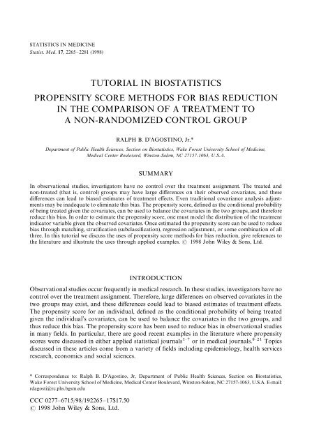
PROPENSITY SCORE METHODS 2275Table V. Comparison of quintile means for variable centimetres at admissionNCentimetres dilatedat admissionMean (SD)Overall No epidural 775 3)95 (1)96)Epidural 1003 2)79 (1)42)After stratification into quintiles based on propensity scoresQuintile 1 No epidural 55 1)93 (1)02)Epidural 263 1)90 (1)03)Quintile 2 No epidural 83 2)55 (1)00)Epidural 236 2)62 (1)11)Quintile 3 No epidural 126 3)00 (1)28)Epidural 193 3)05 (1)19)Quintile 4 No epidural 157 3)54 (1)32)Epidural 162 3)61 (1)42)Quintile 5 No epidural 268 5)40 (1)78)Epidural 50 4)68 (1)19)their propensity scores. We then compared the epidural/no epidural groups on their 15 covariates,after adjusting for their propensity quintile. This was done using a two-way analysis ofvariance model which included main effects for propensity score quintile (coded as a class variablewith 4 degrees of freedom) and epidural use (coded as yes/no). We compared the F-statistic forepidural use after adjustment for propensity score quintile with the F-statistic for epidural useprior to adjustment for propensity score quintile to determine whether balance was achieved afterstratification based on the propensity score. We also examined the two-way interaction of quintileand epidural use. We found that the eight covariates which were significantly different betweenthe two groups prior to stratification, were all non-significantly different after adjustment forpropensity score quintile (see Table IV). Among the interaction terms, only one was significant forthe variable centimetres dilated at first exam (F"3)16, p"0)013). We further examined thisvariable by presenting the quintile means for the epidural and no epidural group (Table V andFigure 1). As can be seen by this table and figure, in the first four quintiles the mean centimetres atadmission are very close, whereas in the 5th quintile the two groups are still somewhat separated.As can be seen in Figure 1, the means for the epidural/no epidural groups cross, and this explainsthe significant interaction between epidural use and propensity score quintile. Nevertheless, ascan be seen both in the table and figure, the two groups are more similar within each propensityscore quintile than they were before stratification. We have included SAS code which was used toestimate the propensity scores and perform the analyses presented here in the Appendix.The investigators had several options for how they would estimate the effects of epidural use onthe rate of Caesarean section use employing propensity scores. One method would be to estimatethe treatment effects separately within each quintile defined by the propensity score and thencombine the quintile estimates into an overall estimate of the treatment effect. An alternativemethod would be to perform a multiple logistic regression with use of Caesarean as the outcomeand epidural use as the independent variable. In this model the propensity score could be 1998 John Wiley & Sons, Ltd.Statist. Med. 17, 2265—2281 (1998)

2276 R. B. D’AGOSTINO, Jr.Figure 1. Comparison of quintile means for variable centimetres (cm) dilated at admissionincluded either as its raw score or the propensity score quintile itself could be included. Inaddition to the propensity score, a subset of the other covariates could be included (such ascentimetres at admission). One advantage of this method is that the final model to estimate thetreatment effect contains fewer covariates than if all the covariates in the propensity score modelhad been used. Therefore traditional diagnostics can be more easily employed to determine the fitof this final model. This was the method employed in this particular application, and the resultsindicated that after adjustment for propensity score (either the raw score or quintile) and a subsetof important covariates, the rate of use of Caesarean sections in the epidural group was stillsignificantly higher than the no epidural group (odds ratio"3)7 with a 95 per cent confidenceinterval from 2)4 to5)7).REGRESSION (COVARIANCE) ADJUSTMENTPropensity scores can also be used in regression (covariance) adjustment. In regression adjustment,the treatment effect, τ, is estimated asτˆ"(½M !½M )!β(XM !XM )where the t and c indicate treatment and control groups. The effect of the background covariatesis adjusted for by subtracting out the second term on the right hand side of the above equation,where β is an estimate of the regression of the responses for the treated and control groups on thebackground covariates. For the reasons stated above, the propensity score is a useful variable inregression adjustments, since one only has to find the regression of the responses on thepropensity scores in the treated and control groups and use this to adjust the final estimate of the 1998 John Wiley & Sons, Ltd. Statist. Med. 17, 2265—2281 (1998)

PROPENSITY SCORE METHODS 2277treatment effect. Roseman finds that if the response surfaces in the treatment and controlgroups are parallel and either linear or non-linear, then the regression adjustment using thepropensity scores reduces the bias in the estimate of the treatment effect. In addition, if onestratifies and then uses regression adjustment within the strata, then this estimator of estimatedtreatment effect appears to be a more efficient estimator than one based on matching alone.Another approach to regression adjustment is to use a large set of background covariates toestimate the propensity score and then take a subset of these covariates and the propensityscore and use them in the regression adjustment. This is the analysis performed above by theACT investigators. This method is also analogous to performing Mahalanobis metric matchingwithin calipers on a subset of the important covariates including the propensity score as discussedabove.As with matching and subclassification, there are examples in the literature where regressionadjustments were used with propensity scores. Here is a brief description of two of them.In Berk and Newton, investigators wished to determine whether new spousal violence wasinfluenced by whether men were either arrested or not arrested for wife-battery. Here thepropensity score was the probability of being arrested and 14 covariates were used to estimate it.Some of these covariates included the suspect’s age, whether the victim was injured, whether thesuspect was drinking, and whether the victim had called the police. The investigators then‘regressed whether or not there was new spousal violence during the follow-up (by the sameoffender against the same victim) on the propensity scores, separately for the arrested and notarrested group’. They found that the arrested and not arrested groups had similar intercepts butdifferent slopes. For the arrested group, the slope was near zero, but for the not arrested group theslope was very steep. This seemed to suggest that subjects who had a high propensity to bearrested, but were not arrested, were more likely to commit violence during the follow-up period.In Muller et al., investigators studied the effects of digoxin in mortality rates in patients aftermyocardial infarction. Here the non-randomized treatment was digoxin. The investigatorscalculated an ‘imbalance risk score’, which appears to be a propensity score, based on 19covariates. The covariates in this model included the subject’s heart rate, age, and whether thesubject had beta-blockers in the previous three weeks. Cox proportional-hazards regression wasused to determine the association between digoxin therapy and survival ‘taking into account theeffects of baseline prognostic factors’. It appears that they ‘took into account’ the baselinedifferences by including a propensity score as a covariate in their model in order to adjust theirfinal treatment effect.One question which may arise when using regression adjustment with propensity scores iswhether there is any gain in using the propensity score rather than performing a regressionadjustment with all of the covariates used to estimate the propensity score included in the model.Rosenbaum and Rubin showed that the ‘point estimate of the treatment effect from an analysisof covariance adjustment for multivariate X is 2 equal to the estimate obtained from a univariatecovariance adjustment for the sample linear discriminant based on X, whenever the samesample covariance matrix is used for both the covariance adjustment and the discriminantanalysis’. Thus, the results from both methods should lead to the same conclusions. However, oneadvantage to performing the two-step procedure is that one can fit a very complicated propensityscore model with interactions and higher order terms first. Since the goal of this propensity scoremodel is to obtain the best estimated probability of treatment assignment, one is not concernedwith over-parameterizing this model. Then when the model for estimating the treatment effect isestimated the investigator can include only a subset of the most important variables and the 1998 John Wiley & Sons, Ltd.Statist. Med. 17, 2265—2281 (1998)

2278 R. B. D’AGOSTINO, Jr.propensity score in the model. This smaller model may allow the investigator to performdiagnostic checks on the fit of the model more reliably than if there were many covariatesincluded in the model.In general, covariance adjustment should be performed with caution. Rubin showed thatcovariance adjustment may in fact increase the expected squared bias if the covariance matrices inthe treated and untreated groups are unequal (that is, if the discriminant is not a monotonefunction of the propensity score). Another difficulty arises when the variance in the treated anduntreated groups are very different (that is, the untreated group variance is much larger than thetreated groups variance). Under these circumstances, one may consider using propensity scoremethods for matching or subclassification, rather than using covariance adjustment.DISCUSSION AND CURRENT RESEARCHIn all the examples stated above, except for Rosenbaum and Rubin, there was no mention of howmissing values on covariates were handled when estimating propensity scores. This is animportant issue in most real data applications. For instance, in the ACT example presentedabove, over 100 subjects would have been excluded from the final analyses based on the fact thatthey were missing covariates included in the propensity score models. The March of Dimes Studyalso had covariates with missing data into the models. Currently, methods are being developed tohandle this problem. which allow for different missing-data mechanisms and use the EMor ECM algorithms to estimate propensity scores.A second area of current research is using propensity scores to estimate treatment effects inclinical trials where subjects drop out prior to the trials completion. Here, propensity scores areestimated as the probability that an individual will complete the trial conditional on their baselineand early outcomes. This work also uses the EM and ECM algorithms to estimate propensityscores with missing data.Propensity scores are being widely used in statistical analyses, particularly in the area ofapplied medicine. Their use should only increase as the cost for randomized clinical trials risesand more investigators turn to observational studies as a means of performing less expensiveresearch. The propensity score methodology appears to produce the greatest benefits when it canbe incorporated into the design stages of studies (through matching or stratification). Thesebenefits include providing more precise estimates of the true treatment effects as well as savingtime and money. This saving results from being able to avoid recruitment of subjects who may notbe appropriate for particular studies. Finally, it is important to note that we are not advocatingthe use of only propensity scores in analyses of observational studies, rather we are encouragingthe use of propensity scores in addition to traditional methods of analysis. The propensity scoreshould be thought of as an additional tool available to the investigators as they try to estimate theeffects of treatments in studies.APPENDIXThe following is a series of SAS code that will estimate propensity scores using the logisticregression procedure in SAS. We first perform a series of t-tests to determine the initial level ofbias between the two groups. Then we calculate propensity scores using stepwise logisticregression. Next, propensity score quintiles are created and then we examine whether the groupsare balanced after adjustment for the propensity score quintiles. 1998 John Wiley & Sons, Ltd. Statist. Med. 17, 2265—2281 (1998)

PROPENSITY SCORE METHODS 2279* This will perform a series of ttests to determine what the initial difference between the* treated and control groups are. Here the variable epidural is the treatment indicator in this* model.proc ttest data"matchset; class epidural;var amladmit cm 1 arom gestage birthwt gender rate chyper phyperheight weight momage insprvt momw momb;* This performs a stepwise logistic regression to estimate propensity scores for each subject.* The variable pr is the propensity score The variable epidural is the treatment indicator in* this model.proc logistic data"matchset nosimple;model epidural"amladmit cm 1 arom gestage birthwt gender rate chyper phyperheight weight momage insprvt momw momb/selection"stepwise;output out"preds pred"pr;* This takes the propensity score and creates quintiles based on the estimated propensity* score;proc rank groups"5 out"r;ranks rnks;var pr;data a; set r; quintile"rnks#1;* This will show the breakdown of subjects by treatment (here epidural) and propensityscore quintile;proc freq; tables quintile*epidural;* This will perform the 2-way anovas to determine whether the propensity score quintiles* removed the initial bias found by the t-tests above.proc glm;class quintile;model amladmit cm 1 arom gestage birthwt gender rate chyper phyperheight weight momage insprvt momw momb"quintile epidural quintile*epidural;ACKNOWLEDGEMENTSThe author wishes to thank Dr. Ellice Lieberman and the investigators from the Active Managementof Labor Trial (National Institute of Child Health and Human Development grant no.R01-HD26813) for use of their data. The author also wishes to thank Dr. Curtis Deutch and theMarch of Dimes Birth Defects Foundation Social and Behavioral Science Research grant for useof their data. The author also wishes to acknowledge the support of his wife Carey and daughtersLucy, Serena and Sophia in this work.REFERENCES1. Rubin, D. B. and Thomas, N. ‘Matching using estimated propensity scores: Relating theory to practice’,Biometrics, 52, 249—264 (1996).2. Bloch, D. A. and Segal, M. R. ‘Empirical comparison of approaches to forming strata: using classificationtrees to adjust for covariates’, Journal of the American Statistical Association, 84,897—905 (1989).3. Ciampi, A., Hogg, S. A., McKinney, S. and Thiffault, J. ‘RECPAM: a computer program for recursivepartition and amalgamation for censored survival data and other situation frequently occurring inbiostatistics. I. Methods and program features’, Computer Methods and Programs in Biomedicine, 26,239—256 (1988).4. Rosenbaum, P. R. ‘Conditional permutation tests and the propensity score in observational studies’,Journal of the American Statistical Association, 79, 565—574 (1984). 1998 John Wiley & Sons, Ltd.Statist. Med. 17, 2265—2281 (1998)

2280 R. B. D’AGOSTINO, Jr.5. Rosenbaum, P. R. and Rubin, D. B. ‘Reducing bias in observational studies using subclassification onthe propensity score’, Journal of the American Statistical Association, 79, 516—524 (1984).6. Rosenbaum, P. R. and Rubin, D. B. ‘Constructing a control group using multivariate matched samplingmethods that incorporate the propensity score’, American Statistician, 39, 33—38 (1985).7. Lavori, P. W. and Keller, M. B. ‘Improving the aggregate performance of psychiatric diagnostic methodswhen not all subjects receive the standard test’, Statistics in Medicine, 7, 723—737 (1988).8. Cook, E. F. and Goldman, L. ‘Asymmetric stratification: An outline for an efficient method forcontrolling confounding in cohort studies’, American Journal of Epidemiology, 127, 626—639 (1988).9. Fiebach, N. H., Cook, E. F., Lee, T. H., Brand, D. A., Rouan, G. W., Weisberg, M. and Goldman, L.‘Outcomes in patients with myocardial infarction who are initially admitted to stepdown units: datafrom the multicenter chest pain study’, American Journal of Medicine, 89, 15—20 (1990).10. Muller, J. E., Turi, Z. G., Stone, P. H., Rude, R. E., Raabe, D. S., Jaffe, A. S., Gold, H. K., Gustafson, N.,Poole, W. K., Passamani, E., Smith, T. W., Braunwald, E. and The MILIS Study Group. ‘Digoxintherapy and mortality after myocardial infarction: experience in the MILIS Study’, New EnglandJournal of Medicine, 314, 265—271 (1986).11. Myers, W. O., Gersh, B. J., Fisher, L. D., Kosinski, A. S., Mock, M. B., Holmes, D. R., Schaff, H. V.,Gillispie, S., Ryan, T. J., Kaiser, G. C. and other CASS Investigators. ‘Time to first new myocardialinfarction in patients with mild angina and three-vessel disease comparing medicine and early surgery:A Cass registry study of survival’, Annals of ¹horacic Surgery, 43, 599—612 (1987).12. Myers, W. O., Gersh, B. J., Fisher, L. D., Kosinski, A. S., Mock, M. B., Holmes, D. R., Schaff, H. V.,Gillispie, S., Ryan, T. J., Kaiser, G. C. and other CASS Investigators. ‘Multiple versus early surgicaltherapy in patients with triple-vessel disease and mild angina pectoris: A Cass Registry Study ofSurvival’, Annals of ¹horacic Surgery, 44, 471—486 (1987).13. Myers, W. O., Schaff, H. V., Gersh, B. J., Fisher, L. D., Kosinski, A. S., Mock, M. B., Holmes, D. R.,Ryan, T. J., Kaiser, G. C. and CASS Investigators. ‘Improved survival of surgically treated patients withtriple vessel coronary artery disease and severe angina pectoris’, Journal of ¹horacic and CardiovascularSurgery, 97, 487—495 (1989).14. Berk, R. A. and Newton, P. J. ‘Does arrest really deter wife battery? An effort to replicate the findings ofthe Minneapolis Spouse Abuse Experiment’, American Sociological Review, 50, 253—262 (1985).15. Berk, R. A., Newton, P. J. and Berk, S. F. ‘What a difference a day makes: an empirical study of theimpact of shelters for battered women’, Journal of Marriage and the Family, 48, 481—490 (1986).16. Czajka, J. L., Hirabayashi, S. M., Little, R. J. A. and Rubin, D. B. ‘Projecting from advance data usingpropensity modeling: an application to income and tax statistics’, Journal of Business and EconomicStatistics, 10, 117—131 (1992).17. Hoffer, T., Greeley, A. M. and Coleman, J. S. ‘Achievement growth in public and Catholic schools’,Sociology of Education, 58, 74—97 (1985).18. Lavori, P. W. ‘Clinical trials in psychiatry: should protocol deviation censor patient data?’, Neuropsychopharmacology,6, (1), 39—48 (1992).19. Lavori, P. W., Keller, M. B. and Endicott, J. ‘Improving the validity of Fh-Rdc diagnosis of majoraffective disorder in uninterviewed relatives in family studies: a model based approach’, Journal ofPsychiatric Research, 22, 249—259 (1988).20. Stone, R. A., Obrosky, S., Singer, D. E., Kapoor, W. N. and Fine, M. J. ‘Propensity score adjustment forpretreatment differences between hospitalized and ambulatory patients with community-acquiredpneumonia’, Medical Care, 33, AS56—AS66 (1995).21. Lieberman, E., Lang, J. M., Cohen, A., D’Agostino, Jr. R., Datta, S. and Frigoletto, Jr., F. D.,‘Association of epidural analgesia with caesareans in nulliparous women’, Obstetrics and Gynecology,88, 993—1000 (1996).22. Rosenbaum, P. R. and Rubin, D. B. ‘The central role of the propensity score in observational studies forcausal effects’, Biometrika, 70, 41—55 (1983).23. Cochran, W. G. and Rubin, D. B. ‘Controlling bias in observational studies: a review’, Sankya, Series A,35, 417—446 (1973).24. Rubin, D. B. ‘Matching methods that are equal percent bias reducing: some examples’, Biometrics, 32,109—120 (1976).25. Rubin, D. B. ‘Using multivariate matched sampling and regression adjustment to control bias inobservational studies’, Journal of the American Statistical Association, 74, 318—324 (1979). 1998 John Wiley & Sons, Ltd. Statist. Med. 17, 2265—2281 (1998)

PROPENSITY SCORE METHODS 228126. Rubin, D. B. ‘Bias reduction using Mahalanobis metric matching’, Biometrics, 36, 293—298 (1980).27. Carpenter, R. G. ‘Matching when covariables are normally distributed’, Biometrika, 64, 299—307 (1977).28. Rubin, D. B. ‘Practical implications of modes of statistical inference for causal effects and the critical roleof the assignment mechanism’, Biometrics, 47, 1213—1234 (1991).29. Hobel, C. J., Youkeles, L. and Forsythe, A. ‘Prenatal and intrapartum high-risk screening. II Risk factorsreassessed’, American Journal of Obstetrics and Gynecology, 135, 1051—1056 (1979).30. Cochran, W. G. ‘The planning of observational studies of human populations’, Journal of the RoyalStatistical Society, Series A, 128, 234—255 (1965).31. Cochran, W. G. ‘The effectiveness of adjustment by subclassification in removing bias in observationalstudies’, Biometrics, 24, 205—213 (1968).32. Frigoletto, F. D., Lieberman, E., Lang, J. M., Cohen, A. P., Barss, V., Ringer, S. A. and Datta, S. ‘Aclinical trial of active management of labor’, New England Journal of Medicine, 333, 745—750 (1995).33. Roseman, L. ‘Using regression and subclassification on the propensity score to control bias in observationalstudies’, unpublished report, Harvard University, 1994.34. D’Agostino, R. B. Jr. ‘Estimating propensity scores when covariates have either ignorable or nonignorablemissing values’, Ph.D. thesis, Harvard University, 1994.35. D’Agostino, R. B. Jr. and Rubin, D. B. ‘Estimating and using propensity scores with partially missingdata’, submitted to Journal of the American Statistical Association, (1977).36. Dempster A. P., Laird N. M. and Rubin D. B. ‘Maximum likelihood estimation from incomplete datavia the EM algorithm (with discussion)’ Journal of the Royal Statistical Society, Series B, 39,1—38 (1977).37. Meng, X. L. and Rubin, D. B. ‘Maximum likelihood estimation via the ECM algorithm: A generalframework’, Biometrika, 80, 267—278 (1993).38. Dawson, R. and D’Agostino Jr., R. B. ‘Propensity-based non-ignorable models for drop-out in clinicaltrials’, submitted to Biometrics (1996). 1998 John Wiley & Sons, Ltd.Statist. Med. 17, 2265—2281 (1998)