A DYNAMICAL MODEL OF OROGRAPHIC RAINFALL

I 

September 1966 R. P. Sarker 555 

A DYNAMICAL MODEL OF OROGRAPHIC RAINFALL 

R. P. SARKER 

Institute of Tropical Meteorology, Poona, India 

ABSTRACT 

A dynamical model for orographic rainfall with particular reference to the Western Ghats is presented. The 

model assumes a saturated atmosphere with pseudo-adiabatic lapse rate and is based on linearized equations. The 

rainfall, as computed from the theoretical model, is in good agreement, both in intensity and in distribution, with the 

observed rainfall on the windward side of the mountain. The model cannot explain the rainfall distribution on the 

lee side, which apparently is not due to the orography considered in the model. 

A simple formula for rainfall intensity has also been found based on continuity of mass and continuity of moisture 

taking into account the convergence or divergence within a thin layer. Further modifications in the dynamical 

model are also suggested. 

1. INTRODUCTION 

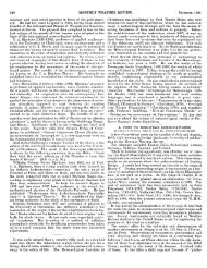
The rainfall over the Western Ghats of India (fig. 1) dur- 

ing the southwest monsoon is often believed to be strongly 

orographic. But as yet there is no quantitative informa- 

tion as to the extent to which the orography of the Western 

Ghats plays a part in causing rainfall. However, the 

effect of topography is fairly well known in the sense that 

precipitation increases with altitude and is greater on the 

slopes facing the prevailing wind than on the lee slopes. 

The rainfall may occur from lifting of saturated air induced 

by other causes as well, viz., horizontal convergence and 

instability. As it is quite likely that rainfall due to orog- 

raphy, convergence, and instability may occur simultane- 

ously in mountainous areas, it is worthwhile to examine the 

role played by orography in causing rainfall and its 

distribution. 

In this paper, we shall examine the amount of orographic 

rainfall and its distribution along the orography with 

particular reference to the Western Ghats. As is well 

known, to explain the amount and distribution of orog- 

raphic rainfall one has to consider the aspects of meteor- 

ology on three different scales. First, there are the large- 

scale synoptic factors which determine the characteristics 

of an air mass which crosses the hills, its wind speed and 

direction, its stability, and its humidity. This aspect has 

been studied by Douglas and Glasspoole [4]. Second, 

there is the microphysics of cloud and rain, which deter- 

mines whether the water which is condensed as cloud will 

reach the ground as rain or snow, or whether it will be 

merely re-evaporated on the leeward side. This aspect 

received the atten tion of Ludlam [ 121, [ 131. Third, and the 

most important, is the dynamics of air motion over and 

around the hill. This determines to what depth and 

through what extent the air mass at each level is lifted. 

This aspect was considered by Sawyer [20] for rainfall over 

the British Isles on the very highly simplified assumption 

that the air is lifted by orography at all levels and to the 

same extent. On this assumption, he computed rainfall 

and compared it with the observed rainfall averaged over 

the Welsh Mountains. An empirical model for computa- 

tion of orographic precipitation is also available in a re- 

port of the US. Weather Bureau [26]. However, a sound 

dynamical model for orographic rainfall based on the 

theories of air flow over mountains is still lacking. We 

propose to give here a model for the orographic rainfall 

over the Western Ghats. This model gives the amount 

of rainfall due to lifting caused by orography and also ac- 

counts for the variation of rainfall along the slope. 

2. THE DYNAMICAL MODEL 

We consider below how far the moisture-laden air is 

lifted by the Western Ghats. In a previous paper the 

author [19] investigated the mountain wave phenomena 

over the Western Ghats and showed that the air mass 

during the winter months has sufficient stable stratifica- 

tion to produce lee waves. The air current near the 

Western Ghats during the southwest monsoon is sub- 

stantially different. In this season, the air mass does not 

have that much stable stratification. It is more or less 

neutral for moist adiabatic processes or even sometimes 

unstable in some layers. The wind is westerly below and 

easterly aloft. Generally, the westerly wind increases 

from 10 kt. at the surface to about 30-40 kt. between 1 

and 2 km. and then gradually decreases and becomes 

easterly at about 6-7 km. On a strong monsoon day, 

the westerly wind may extend up to 10 km. as well and 

also may be considerably stronger. Moreover, it has 

often a secondary maximum in the layer 5-6 km. The 

linearized perturbation equation is not quite suitable for 

such an air stream as the differential equation does have 

a singularity at the level where the westerly wind changes 

to easterly (i.e., U=O). However, confining our attention 

to low levels only (6-7 km.), we may still get a satis-

556 MONTHLY WEATHER REVIEW Vol. 94, No. 9 

12 

730 740 75" 7bo 770 

0 

9 

8 

7 

b 

15 

14 

13 

FIGURE 1.-Map of the Western 

Ghats. Contours are at 300-m. 

intervals above 300 m. The 

broken rectangle indicates the area 

under study. In the area, the 

open circles indicate locations of 

the rain-reporting stations. The 

z,z profile of the area within the 

rectangle is represented by equa- 

tion (8).

Sepetrnber 1966 R. P. Sarker 557 

factory approximate solution, as the motion within 6-7 

km. is not much affected by the flow pattern above (Palm 

and Foldvik [17], Corby and Sawyer [l], and Sawyer 1211). 

We, therefore, base our dynamical model on the linearized 

equations. 

We assume a two-dimensional flow in the vertical plane 

xz, with the z axis vertical and the z axis from west to 

east, i.e., in the direction of the undisturbed wind. In the 

two-dimensional flow the mountain is assumed to have an 

infinite extent in the y direction (south to north) and the 

flow is entirely cver the mountain. This assumption is 

not far from reality as the Western Ghats extends for 

about 1500 km. in the S-N direction. We assume further 

(i) the undisturbed quantities are functions of z only, 

(ii) the perturbation quantities are small so that their 

product and higher-order terms are neglected compared 

to the undisturbed quantities, (iii) the motion is non- 

viscous and laminar, (iv) the earth's rotation is neglected, 

and (v) the motion is steady. 

The basic equations are two equations of motion, equa- 

tion of state, adiabatic equation, and equation of con- 

tinuity. Starting with these equations and after lineari- 

zation and elimination, we find the following differential 

equation for the vertical perturbation velocity (Sarker 

1191) : 

where 

and the vertical velocity w is given by 

w(z, z) =Re We eikZ exp eGz)=Re (:>"2 W. eta (3) 

In the above 

U, T, p=undisturbed wind, temperature, and density 

respectively . 

g=acceleration due to gravity. 

r*=adiabatic lapse rate, dry or moist. 

y=actual lapse rate in the undisturbed atmosphere= 

-dT/dz. 

R=gas constant. 

x = d(S- Rrgv *> 

Re=Real part of( ). 

. 

The quantity x becomes for a dry adiabatic lapse rate 

the ratio c,/c,=1.4 of specific heat at constant pressure to 

specific heat at constant volume. On the other hand for 

a moist adiabatic lapse rate, it varies with height. 

Equation (1) gives the vertical velocity for a sinusoidal 

ground profile from which is obtained the vertical velocity 

for a smooth profile by the method of Fourier Integral. 

The solution of equation (1) depends upon the behavior 

of j(z) with z. We shall solve this equation for the condi- 

tion during the monsoon. The monsoon air current is 

moist so that we assess the stability of the atmosphere 

relative to the saturated adiabatic lapse rate. We thus 

replace y* by ym the pseudo-adiabatic lapse rate. On 

examination of the actual lapse rate, it is seen that 

the atmosphere is more or less neutral or even some 

times slightly unstable as compared with the pseudo- 

adiabatic lapse rate. We, however, assume in our model 

a saturated atmosphere in which both the environment 

and the process have the pseudo-adiabatic lapse rate. 

Thus the atmosphere in our model has neutral stability 

and this is consistent with our assumption of laminar 

flow. The first term of the expression for f(z) in (2) 

then vanishes and the second term, viz, the shear term, 

is the most important term as compared to the remaining 

three terms. 

The variation of f(z) with height can be seen in figures 

3, 9, 12, 15, 19, 22. It is seen thatf(z) is positive in the 

lowest layer, it is negative in some middle layer corresponding 

to positive values of d2U/dz2, and again becomes 

positive above. We are, therefore, obliged to take in 

our model a negative value of f(z) in the middle layer. 

We accordingly divide the atmosphere into three layers 

as follows: 

f(z)=Z: when zH 

The differential equation (1) for the three layers thus 

becomes: 

Lowest Layer: 

--?i-+[l~-k2]W,=0 

d2Wi for zSzo 

dz 

Middle Layer: 

Upper Layer: 

3. SOLUTION FOR WESTERN GHATS 

We now solve equations (5)-(7) for the Western Ghats 

profile. The location map of Western Ghats is shown 

in figure 1. The Ghats extends for about 1500 km. in the 

north-south direction. We have restricted our present 

investigation to the portion marked by the broken rec- 

tangle. For this area, the height on an average, rises 

from west to east gradually to 0.8 km. in a distance of 

65 km. and then ends in a plateau of average height 0.6 

km. The average west-east vertical cross section of this 

portion of the Ghats is shown schematically at the bottom 

(5) 

(7)

558 MONTHLY WEATHER REVIEW Vol. 94, No, 9 

of figure 7 and suceeding rainfall rate graphs and can be 

represented by the equation 

where rS(z) is the elevation of the ground surface at the 

level z=--h with the numerical values h=0.25 km., 

a=18.0 km., b=0.52 km., and ar=(2/s)X0.35 km. As 

mentioned earlier, we solve first equations (5)-(7) for 

a sinusoidal ground profile of wave number k and then 

generalize the solution for an arbitrary mountain by the 

method of Fourier Integral. 

The solutions of equations (5)-(7) are 

where 

} W2(z, k)=Ccosh pz+D sinh pz (9) 

Wl(z, k) =E cos uz+F sin vz 

W3 (2, k) =Ae +"+ BeAZ 

V= Jl:-k2, p= Jk2+1g, A=Jk2-l,Z (94 

The constants A, B, C, D, E, F are to be found from the 

boundary conditions. 

At the upper boundary, we require that energy of the 

perturbation must remain finite at great heights, so that 

W3+0 as z--. Also at the interfaces z=zo and Z=H 

we require that both vertical velocity and pressure are 

continuous. These conditions require that W and dW/dz 

are continuous at the interfaces. Applying these conditions 

we have the following expressions for Wl, Wz, W,: 

-5 sinh p(zo--H) 

cc 

sinh p(zo--H)-- cosh p(zo--H) 

A 

Wz(z, k)=Ae-'I cosh p(z-H)-- sinh p(z-H) 

P 

w&, k) =Ae-Az J 

A is to be found from the lower boundary condition. At 

the lower boundary, we require the flow to be tangential 

to the surface. For the profile (8) this condition is 

Wl(xJ--h) = U(rs)b{,(x)/bz so that the linearized lower 

boundary condition is 

The solution satisfying this condition is 

x 

fi 

where 

~ ~ ( k)=cos 2 , u(z-zo) cosh p(zo-H)-- x sinh p(zo-H) 

{ cc 

and 

-5 cc cosh p(zo-H)} 

-E cc cosh p(z,-H) 

Now, the value of the integral in (12) depends upon the 

behavior of the function of A(k) in the range of integration. 

If A(k) vanishes in the range of integration, then the 

integral becomes an improper integral. In that case, we 

define the value of the integral as the Cauchy principal 

value and we see that W1,2,3(~, z) can be adequately 

divided into two parts-the wave part and the forcing 

part. The wave part corresponds to the values of k where 

A(k) vanishes. However, in our present model we have 

seen that for all the cases studied here, there is no wave 

on the lee side of the mountain. It is seen that A(k) does 

not vanish for any real value of k and it increases very 

rapidly as le increases. The solution of (12) is thus only 

the forcing part. It is difficult to get an exact value of 

the integral in (12) and by following Scorer [22], [23] the 

approximate solution is obtained by putting k=O in 

[AI, 2,3(z, k)]/A(k). The approximation as Scorer recog- 

nizes, and as Sawyer [21] points out, is not good near the 

origin, but we are helped here to draw the streamlines as 

the flow is smooth. However, the vertical velocity as 

obtained from the approximate solution is not strictly 

representative of the actual vertical velocity in the 

neighborhood of x=O. 

The approximate solution is 

1" e-ak (ab-i $)


where A is the value of A(k) at k=O. When we put k=O, 

we get the following values of X, 1.1, v from (sa) 

A=&&, p=12, v=ll (14) 

There has been considerable controversy as to the choice 

of the sign of X. Scorer in all his papers chose the positive 

sign. The rest of the workers in this field (viz., Corby and 

Sawyer [2], Palm [16], Queney et al. [HI) have shown that 

the negative sign for X is the appropriate choice which 

places the lee waves downstream. This choice also has 

been confirmed by Crapper [3] by a rigorous analytical 

treatment. We have, accordingly, chosen the negative 

A= -iZ3 in (14). With this choice the values of A1,2, 3(2, 0) 

and A in (13) are as follows: 

A=COS Zi(h+zo) cash Zz(zo-H) { 

2 

ti 2 sinh Z2(zo--H) 

12 

{ sinh Z2(z0-H)+i 2 I cosh 12(z,,-H)} 

Expression (13), with the values of A1,2,3(2,0),A in (15), 

when multiplied by (p,/pJU2 gives the vertical velocity 

due to the mountain. The corresponding displacement 

Sa(z,z) of the streamline above its original undisturbed 

level z is given by 

In the above ps is the undisturbed density of air at the 

ground and pz is the density at a level z above the origin. 

227-347 M L - 3 

12 

4. COMPUTATION OF RAINFALL 

We now make use of the vertical velocity obtained 

from our dynamical model to compute rainfall and its 

spatial distribution along the orography of the Western 

Ghats (fig. 1). 

As mentioned earlier, we assume a saturated atmosphere. 

Rainfall for pseudo-adiabatically ascending air 

has been computed by many authors; viz., Fulks [5], 

Showalter [24], Kuhn [9], and Thompson and Collins [25]. 

Fulks and Showalter both assume that there is no divergence 

at the bottom and the top of a layer. As will be 

seen from the vertical velocity profiles to be presented, 

this assumption is not true in our case. While Thompson 

and Collins take initial unsaturated conditions into 

account, Kuhn takes into account the divergence or 

convergence at the bottom and top of a layer. However, 

it appeared to the author that in all the above formulas, 

the continuity of mass of air within the layer has been 

ignored. We accordingly derive below a formula for 

rainfall computation based on simple physical considerations 

so as to take into account the continuity of mass also. 

Let Az be the thickness of a column of air of unit cross 

section. If po,pl be the density of dry air at the bottom 

and top of the layer and Wo,Wl be the corresponding 

vertical velocities, then the mass of air entering at the 

bottom of the layer is powo and the mass leaving the top is 

plWl. Now if poWofplWl there is either divergence or 

convergence (two dimensional) in the layer. If powo> 

plWl there is divergence so that the mass of air that leaves 

the column sideways is poWo-plWl and considering that 

the thickness of air column is small, we can with sufficient 

accuracy assume that the mass leaves the column sideways 

at its middle point. Thus if xo, z1 be the humidity mixing 

ratios,of saturated air at the bottom and top of the layer, 

and 2' that at the middle, the quantity of moisture that 

enters the column is poWozo and the quantity that leaves 

is [p,Wlq+ (poWo-plWl)d]. Thus, assuming that the 

rate of precipitation is equal to the rate of condensation, 

we find that the amount of rainfall from the column is 

[PoWo~a- Cm'CY1s +(PoWo-Pl'CYl)s' 11 

expressed in proper units. If density is expressed as 

kgm.-3, humidity mixing ratio as gm. kgm.-' and vertical 

velocity as cm. set.-', then the rainfall intensity is 

1=0.036[p0W0x0- { pl'CYla +(poWo-pmWl)x'~] mm./hr. 

= 0.036[ po Wo( so - z') + pl Wl (2' - XJ ]mm./hr. 

(17) 

As a very good approximation we could replace xf by 

the mean value (x0+x1)/2 of the column. Formula (17) 

is also the expression for rainfall intensity when there is 

convergence in the layer, that is, when plWl>poWo. 

The above simple formula is believed to be an improve- 

ment upon the existing formulas for computation of rain- 

fall intensity, as it considers, apart from continuity of 

moisture, t8he continuity of mass also when there is 

divergence or convergence witshin a layer. We have

5 60 MONTHLY WEATHER REVIEW Vol. 94, No, 9 

applied this formula to compute rainfall intensity for 

500-m. thicknesses from surface to 6-7 km. up to which 

our dynnmical model for vertical velocity is believed to be 

valid. 

DOWNWIND EXTENSION OF PRECIPITATION 

The rain that falls from a particular layer will not 

necessarily fall vertically below the layer, for the air- 

stream will carry it downstream. Any realistic model for 

space distribution of precipitation must take this into 

account. This effect on the appearance of precipitation 

patterns on a radar screen and on the size dispersion of 

raindrops has been discussed by Marshall [ 141, Langleben 

[lo], Gunn and Marshall [7] and Mason and Andrews 

[15]. Their discussions have dealt mainly with the 

generating cells moving with the wind velocity at the 

level of the generating cell. We consider below the 

horizontal extension of the precipitation along the wind 

in the case of fixed generating cells. 

If U(z) be the horizontal wind at the level z and p be 

the terminal velocity of the precipitation element (which 

is a snow flake above the freezing level and a melted 

droplet below the freezing level), then the horizontal 

distance x traveled by the precipitation element created 

at an anchored generating cell at the level zo in falling to 

the level z is given by 

1 

x=- P JZo U(2)dz 

The above formula is derived on the two assumptions 

that (i) the rate of descent of the precipitation element is 

constant and is equal to its terminal velocity, and (ii) the 

precipitation element moves horizontally with the speed 

of the wind. The integral in (18) is equivalent to the 

area bounded by the graph of U(z) against z, the z-axis 

and the levels zo and z. 

TERMINAL VELOCITY OF PRECIPITATION ELEMENTS 

We have assumed a pseudo-adiabatic condition in our 

model which places the freezing level at a particular 

height. This level generally lies at 5.5 km. This may, 

of course, vary from one case to another. The precipita- 

tion element above the freezing level is a snow flake and 

a melted droplet below. The terminal velocities accord- 

ingly are different above and below the freezing level. 

The orographic rainfall, as will be seen later, generally 

varies from 2-8 mm./hr. According to Kelkar [8] the 

most probable drop-diameter corresponding to this rate 

of precipitation is 1.00-1.25 mm. The terminal velocity 

corresponding to this drop-diameter is 4.5 m. set.-' (Gunn 

and Kinzer [6], reproduced by List [ll]) in the liquid 

phase and 1.00 m. sec.-' in the snow phase (Langleben 

[lo11 

Using these terminal velocities and the given wind 

profile we construct the trajectory which a precipitation 

element starting at a particular level will follow to reach 

the ground. 

5. NUMERICAL COMPUTATION 

We have performed numerical computations for seven 

cases when the monsoon was strong as well as weak. 

We have taken both individual days as well as a few 

spells of 3 to 4 days. For the undisturbed wind and 

temperature we have taken data of Santacruz (19'07' 

N., 72'51' E.) which is a sea level station on the windward 

side of the Western Ghats at a distance of 65 km. from 

the crest. For temperature we have, of course, taken 

the pseudo-adiabatic line through the surface dew point, 

or surface dry bulb, or mean in order to be realistic in 

regard to the actual distribution of temperature and dew 

point. The wind and temperature distributions are given 

in figures 2, 8, 11, 14, 18, 21 and those of f(z) in figures 

3, 9, 12, 15, 19, 22. The continuous line forf(z) shows 

its actual distribution and the dashed lines show the 

? 

E 

Y 

c 

9 

8 

7 

6 

c 5 

I 

2 

YI 

I 

4 

l t I I I A,, 

240 250 260 270 280 290 300 

TEMPERATURE ('A.) 

I 1 I I I I 1 

-10 -5 0 5 10 IS 20 

WIND (m./sec.) 

FIGURE 

2.-Average wind and temperature profiles for July 5, 1961 

(case I). Positive wind is westerly, negative is eaeterly.

September 1966 R. P. Sarker 5 61 

TABLE I.-constant values taken for f(z) for the diferent layers, and 

boundary heights of the layers, jar the cases studied 

No. 

I 

I1 

111 

IV 

V 

VI 

VI1 

layer 

July5, 1961 __._.. 2.50 5.00 0. 36 -0.25 0. 16 

June 25, 1961.. .. 3.25 5.25 0.25 -0.15 0. 25 

July G9, 196X.. 1.75 3.25 0.60 -0. 15 0. 16 

July 11-12, 1958. 2. 50 4. 00 0.36 -0.10 0. 16 

July 21, 1959 ___.. 2.50 4.00 0.30 -0.16 0.13 

July 2-4 1960--.. 2.00 4. 00 0.45 -0.075 0.075 

July 4-6: 195L.I 2.25 _._......__. 0.49 .-~ ......_.. 0. 16 

constant values taken for f(z) at the different levels. 

The values of the parameters l:, Zz, Zz, and z,,+h, Hfh are 

given in table 1. We now discuss the difl'erent cases. 

CASE I-JULY 5, 1961 

In figure 2 is given the relevent undisturbed wind and 

temperature distribution for Case I, July 5, 1961. The 

surface wind is 8 m./sec. The maximum wind is 20.5 

m./sec. at a level 1-1.5 km. The wind then decreases to 

7.5 m./sec. at 4 km., and again increases to 10.5 m./sec. 

at 6 km., then decreases and becomes easterly at 8.5 km. 

The surface temperature is 300' A. and the surface dew 

point is 298' A. In the model, we have assumed for temperature 

the pseudo-adiabatic line through the surface 

dew point 298' A. The relative humidity available up to 

4.3 km. (600 mb.) varies from 80 to 100 percent. 

The distribution of the functionf(z) with z is shown in 

figure 3, and the values of dU[dz and dzU/dz2 are given in 

figure 4. dzU/dz2 is negative from surface to 2.5 km. It 

is then positive up to 5 km. and is then again negative. 

The functionf(z) is positive up to 2.5 km., is negative in 

the layer 2.5 to 5.0 km., and is then positive. Accordingly, 

as mentioned earlier, we have divided the atmosphere 

into three layers. The layer surface to 2.5 km. has the 

constant value 0.3.6 km.-2 forf(z), the layer 2.5-5 km. has 

the constant value -0.25 km.-2, and the upper layer has 

the constant value 0.16 km.-2 This last value was chosen 

to represent f(z) in the entire upper atmosphere, as this 

will not affect the motion below. The streamlines for 

this case are given in figure 5. It is seen that the crest of 

the streamlines tilts upstream. The motion descends 

beyond the top of the mountain. Descending motion 

-1.0 -0.8 -0.6 -0.4 -0.2 0 0.2 0.4 0.6 0.8 1.0 1.2 1.4 

f( I)( km-2) 

FIGURE 3.-Profile of f(z) for July 5, 1961 (case I).

562 MONTHLY WEATHER REVIEW Vol. 94, No. 9 

1 I I I I 

-I5 -10 -5 0 5 10 15 20 

FIGURE 4.-Profiles of dU/dz (rn.sec.-l km.-*) and daUldz2 (m.sec.-1 

km.-2) for July 5, 1961 (case I). 

starts even earlier in the upper level. The distribution 

of the perturbation vertical velocity with height z and 

horizontal distance z is depicted in figures 6 (a), (b). 

The ascending motion starts before the mountain is 

reached and the magnitude in general increases as one 

proceeds along the mountain toward the peak. This 

continues up to z=-5 km., i.e., 10 km. from the crest. 

The magnitude then decreases till 2=3, i.e., 2 km. from 

the crest, after which ascending motion is replaced by 

descending motion. Also we see that in general, vertical 

velocity first increases with height and then decreases and 

then becomes negative; that is, an ascending motion below 

is replaced by descending motion above. Also the level 

of non-divergence, i.e., maximum vertical velocity, grad- 

ually decreases as we proceed from the coast toward the 

crest of the mountain. The variation of vertical velocity 

along the direction 2 itself suggests that rainfall along the 

orography cannot be uniform. 

The rainfall distribution along the orography is given 

in figure 7. The solid line shows the observed intensity 

and the dashed line represents the orographic intensity as 

obtained by our model. For observed rainfall we have 

taken the section 20 mi. north-south of the Bombay- 

Poona region and for this section the only stations available 

are: Bombay at the coast; Pen and Roha about 20-25 km. 

from the coast; Khandala and Lonavla at 13 and 10 km. 

on the windward side from the crest, respectively; and 

60 

60 

z(km.) 

-80 -40 0 40 80 

DISTANCE (km.) 

I 

I 

FIQURE 5.-Streamline displacements set up by the mountain on 

July 5, 1961 (case I). 

Vadgaon and Poona on the lee-side plateau at distances 

of 5 and 40 km. from the crest (see fig. 1). 

In figure 7, the theoretically computed orographic 

rainfall at the coast is 1.2 mm./hr. where the actual rain- 

fall is 6.2 mm./hr. The highest computed orographic 

rainfall is 8.4 mm./hr. and the highest observed rainfall is 

12.2 mm./hr. There is very close agreement between the 

positions of the peaks of the observed and the theoretically 

computed rainfall. Both the observed and orographic 

rainfall fall sharply beyond the peak rainfall. At the top 

of the mountain the theoretically computed rainfall is 

2 mm./hr. and the observed value is 4 mm./hr. Beyond 

this the computed orographic rainfall is little and is nil 

beyond 10 km. from the crest. The observed peak is at 

a distance of 10 km. from the crest and the theoretically 

computed peak is 12 km. from the crest. The theoret- 

ically computed peak value is 69 percent of the observed 

peak. 

CASE II-JUNE 25, 1961 

For Case 11, June 25, 1962 the relevant average wind


- I I’l! I 

3L-11 \! ‘ 

VERTICAL VELOCITY (cm./sec.) 

-5 0 5 10 15 20 25 30 

VERTICAL VELOCITY (cm./sec.) 

FIGURE 6.-Perturbation vertical velocity W (cm./sec.) profiles at 

different distances x along the orography on July 5, 1961 (case I). 

x= 5 is the crest of the mountain. (a) Profiles for - 100 km. 5 

z I - 10 km., x= - 60 is the coastal position; x= - 80, - 100 are 

points at sea. (b) Profiles for -5 km.

- 

€ 

Y 

8- 

7 - 

6- 

5- 

z4- 

I 

(3 

- 

Ly 

I 

3- 

2- 

1 - 

260 270 280 290 300 310 

TEMPERATURE ("A.) 

I I I I I I 

0 5 10 15 20 25 


FIGURE 8.-Average wind and temperature profiles for June 25, 1961 

(case 11). 

(observed as well as computed orographic) falls off sharply 

beyond the peak. At the top of the mountain rainfall 

(comput,ed orographic as well as observed) is 3 mm./hr. 

The computed rainfall is nil beyond 15 km. from the top. 

Moreover, the rainfall beyond the crest results only from 

spillover as there is no ascending motion beyond the top. 

CASE Ill-JULY 6-9, 1963 

For Case 111, the rainfall spell of July 6-9, 1963, the 

average wind and temperature distributions are given 

in figure 11, which is based on the data of July 5 (1730 

IST) to July 8 (1730 IST). We have ensured that the 

processes during this period were more or less constant. 

The wind speed increases from 6 m./sec. at the surface 

to 15.5 m./sec. at 1 km. It then decreases to 11 m./sec. 

at 2.5 km., again slowly rises to 12 m./sec. at 4 km., and 

then decreases to 2 m./sec. at 7 km. The surface tem- 

MONTHLY WEATHER REVIEW 

\ 

z(km.) 

Vol. 94, No. 9 

1 1 

-0.4 -0.2 0 0.2 0.4 

f(z)(km.-* ) 

FIGURE 9.-Profile of f(z) for June 25, 1961 (case 11) 

perature is 298" A. and the dew point 297" A. We have 

taken the pseudo-adiabat through 297" A. The relative 

humidity varies from 90 to 100 percent up to 600 mb. 

(4.3 km.). The f(z) profile (fig. 12) is negative in the 

layer 1.75 to 3.25 km. corresponding to positive values of 

d2U/dz2. The constant values taken for f(z) are 0.60 

km.-2 up to 1.75 km., -0.15 km.-2 up to 3.25 km., and 

0.16 km.+ above 3.25 km. The streamline and vertical 

velocity profiles have the same pattern as in the first 

case. However the descending motion starts earlier. 

Ascending motion starts well before the mountain is 

reached. It increases and then begins to decrease from 

15 km. from the peak. Beyond x=1 km. the motion 

descends at all levels.


lk, / 

0 .I- '- 

-60 -40 -20 0 20 40 


FIGURE 10.-Rainfall distribution for June 25, 1961 (case 11). See 

legend for figure 7. 

In figure 13, the computed orographic rainfall is 1.4 

mm./hr. at the coast and the observed rainfall is 2.4 

mm./hr., that is, the orographic rainfall is 60 percent of 

the observed value. The maximum rainfall is 7.8 mm./hr. 

and the computed maximum orographic rainfall is 5.9 

mm./hr., i.e., 76 percent of the observed rainfall. The 

computed orographic peak occurs 14 km. from the top 

of the mountain and the observed peak, 10 km. Both 

the rainfall curves fall sharply beyond their peak. The 

computed orographic rainfall at the top of the mountain 

is nil, whereas the actual rainfall is 2.8 mm./hr. In this 

case there is no spillover, for, in the model, the ascending 

motion stops about 4 km. before the top is reached. 

CASE IV-JULY 1 1-1 4, 1965 

The relevant data of wind and temperature are given 

in figure 14 for Case IV, the rainfall spell of July 11-12, 

1965. The wind speed increases from 8 m./sec. at the 

surface to 18.5 m./sec. at 2.0 km. It then decreases to 

15 m./sec. at 3.5 km., rises to 16 m./sec. at 4.5 km., and 

then decreases and becomes easterly at 8.5 km. The 

surface dry bulb temperature is 299" A. and the dew point 

is 298"A. We have taken the pseudo-adiabatic line 

through 298OA. The relative humidity varies from 85 

to I00 percent. The-f(z) profile (fig. 15) is negative in 

the layer 2.5 to 4.0 km. corresponding to positive values 

of d2U/dz2. The constant values of f(z) chosen are 0.36 

km.+ up to 2.50 km., -0.10 km.+ up to 4.0 km., and 

0.16 km.-2 above. The streamline and vertical velocity 

distributions have patterns similar to the other cases. 

- 

a 

7 

6 

5 

E 

Y - 

s4 

: I 

3 

2 

1 

\ \ 

I '\ 

I I 


I I I I 1 

0 5 10 15 20 


FIGURE 11.-Average wind and temperature profiles for July 6-9, 

1963 (case 111). 

1 z (kd 

6 1 f 

5 

-0.4 -0.2 0 0.2 0.4 0.6 0.8 1.0 1.2 

Yz) (krn.-*) 

FIGURE 12.-Profile of f(z) for July 6-9, 1963 (case 111).

5 66 MONTHLY WEATHER REVIEW Vol. 94, No. 9 

Of I- 

-60 -40 -20 0 20 40 


FIQURE 13.-Rainfall distribution for July 6-9, 1963 (case 111). 

See legend for figure 7. 

As usual, the ascending motion starts well before the 

mountain is reached. It increases, then decreases, and 

beyond c=O, i.e., 5 km. from the top, the motion is 

descending. Along the vertical it first increases, then 

decreases, and then becomes negative. 

Both the computed orographic and the observed rainfall 

(fig. 16) at the coast are 2.2 mm./hr. This time the entire 

rainfall from the coast to the position of rainfall peak seems 

to be due to orography. However, the computed maxi- 

mum orographic rainfall (8.8 mm./hr.) falls short of the 

observed peak rainfall by 1.0 mm./hr. The computed 

orographic peak value is thus 90 percent of the observed 

peak value. Also the computed orographic peak occurs 3 

km. before the observed peak. The computed orographic 

rainfall falls off very sharply beyond its peak, whereas the 

fall of observed rainfall is not so sudden. The computed 

orographic rainfall at the crest is nil, whereas the ob- 

served value is near 5 mm./hr. The spillover effect is nil 

as descending motion starts from 5 km. before the top is 

reached. 

CASE V-JULY Pi, 1959 

The relevant wind and temperature data for Case V, 

July 21, 1959, (not illustrated) show that the wind speed 

increases from 9 m./sec. at the surface to 16 m./sec. at 2 

km. It then decreases to 11 m./sec. at 3.5 km. The wind 

then again increases with a secondary maximum of 12 

m./sec. at 4.5 km. after which it decreases and gradually 

becomes easterly at 8.5 lrm. The surface dry bulb tem- 

perature is 299' A. and the dew point is 298" A. In the 

model we have taken the pseudoadiabat through 298" A. 

The relative humidity values available vary in the range 

85 to 95 perc,ent. Thef(z) profile is negative in the layer 

'\ 

1 

E 

9 - 

8- 

7 - 

6 - 

z5- 

Y 

v 

2 

y1 

I 

4- 

3- 

2- 

1 - 

I 

I I 

\ 

\ 

\ ' 

\ I 

2 50 260 270 280 


290 300 

-5 0 5 10 15 20 


FIGURE l4.-Average wind and temperature profiles for July 11-12, 

1958 (case IV). 

2.5 km. to 4 km. corresponding to positive values of 

d2U/dz2. The constant values of f(z) are taken as 0.30 

km.-2 from surface to 2.5 km., -0.16 km.? up to 4 km., 

and 0.13 km. above (table 1). 

The streamline and vertical velocity patterns are similar 

to those of the'other cases. The ascending motion in- 

creases as we move toward the crest up to x= - 10 (maxi- 

mum is 32 cm. set.-') after which it decreases and de- 

scer.ds at s=2 krn., i.e., 3 km. before the crest is reached. 

Also the ascending motion first increases with height then

Sepfember 1966 R. P. Sarker 567 

I 

I 

z(km.) 

a 

7 

6 

- 

1 

f(z) 

5 

4 

2 

(km.-2) 

FIGURE 15.-Profile of f(z) for July 11-12, 1958 (case IV). 

decreases and becomes negative. Also up to x= -20 km. 

from the coast the motion ascends at all levels up to 7 km. 

Then the descending motion starts at high levels and the 

level of change-over from ascending to descending motion 

goes down gradually as one moves along the orography 

until the motion is entirely descending at x=2. 

The computed orographic and the observed rainfall are 

in very good agreement (fig. 17). At the coast the ob- 

served rainfall is 1.8 mm./hr. and the computed orographic 

rainfall is 1.7 mm./hr., i.e., 94 percent of the actual. The 

computed orographic rainfall peak slightly exceeds the 

actual peak; viz., the computed orographic maximum is 

9.0 mm./hr. whereas the actual maximum is 8.5 mm./hr. 

Also the position of the two peaks is the same. However, 

in this case the position and magnitude of the peak value 

of actual rainfall is a bit subjective as the rainfall of 

Lonavla (which is very near Khandala) is not available. 

The computed orographic rainfall at the crest of the moun- 

tain is 1 mm./hr. whereas the observed rainfall is 3 mm./ 

hr. The spillover effect is practically nil. It appears the 

entire rainfall is due to orography on the windward side. 

227-347 0-6- 

10 

9 

8 

7 

-2 

z 

\ 6 

E 

E 

- 5 

w 

I- 

2 4 

a 

: 

LL3 

z 

2 2 

't 

I 

\ 

I I 

\ 

I 

\ 

'. 

-60 -40 -20 0 20 40 


FIGURE 16.-RainfalI distribution for July 11-12, 1958 (case IV). 


2 4 

a LL 

53 

U 

OL 

2 

1 

-60 -40 -20 0 20 40 45 


FIGURE 

l'l.-Rainfall distribution for July 21, 1958 (case V). See 

legend for figure 7.

568 

8 

7 

6 

2 

1 

0 

2 50 260 2 70 280 290 3 00 


I 1 I I I 1 

0 5 10 15 20 25 


FIGURE 18.-Average wind and temperature profiles for July 2-4, 

1960 (case VI). 

CASE VI-JULY 2-4,1960 

I The relevant average temperature and wind data are 

given in figure 18 for Case VI, the rainfall spell of July 24, 1960. The wind speed increases from 7 to 14 m./sec. at 1 

km. It then decreases to 10 m./sec. at 3 km. after which 

it decreases slowly to 5 m./sec. at 8 km. and becomes 

easterly at 10.5 km. d2U/dz2 is negative up to 2 km., then 

it is positive up to 4 km., and then either negative or zero 

above. The surface dry bulb temperature is 300' A. and 

the dew point is 299' A. In the model we have taken the 

pseudo-adiabat through 299' A. Relative humidity is in 

the range 85-90 percent. Figure 19 showsf(z) is negative 

in the layer 2 to 4 km. corresponding to positive values of 

d2U/dz2. The constant values taken for f(z) are 0.45 

km.-2 up to 2 km., -0.075 km.-2 up to 4 km., and 0.075 

km.-2 above (table 1). 

MONTHLY WEATHER REVIEW 

I 

I 

1 

I 

-J 0.075 

Vel. 94, No. 9 

L 

I 

1 

-0.4 -0.2 0 0.2 0.4 0.6 0.8 

f(z) (krn-') 

FIQURE 19.-Profile of f(z) for July 2-4, 1960 (case VI). 

The streamline and vertical velocity patterns are sim- 

ilar to the other cases. However, amplitude and vertical 

velocity seem to be slightly higher. The vertical velocity 

gradually increases along the orography until x= - 10 km. 

after which it decreases. The maximum velocity is 31 

cm./sec. Also the vertical velocity increases first with 

height, reaches a maximum and then decreases, and then 

becomes negative at higher levels. The level of change- 

over from ascending to descending motion goes down 

gradually as we proceed toward the crest and the motion 

is entirely descending beyond x= - 1 km., Le., from 4 km. 

before the crest is reached. 

The agreement between observed rainfall and computed 

orographic rainfall is good (fig. 20). The observed rain- 

fall at the coast is 2.7 mm./hr. and the computed oro- 

graphic rainfall is 2.2 mm./hr., i.e., 81 percent of observed 

rainfall. The computed maximum orographic rainfall is 

9.5 mm./hr., which is equal to the maximum observed 

rainfall. Also the positions of the peaks are at the same 

I 

I 

I 

I

September 1966 R. P. Sarker 5 69 

9 L I 

\ I 

I 

'\ I 

-60 -40 -20 0 20 40 


. FIGURE 20.-Rainfall distribution for July 2-4, 1960 (case VI). 


point or differ at most by 2 km. The agreement even 

after the rainfall peaks is dso good for another 8 km. 

The computed orographic rainfall at the crest is zero 

whereas the observed rainfall there is 2.8 mm./hr. 

CASE VII-JULY 4-6, 1958 

Case VII, the rainfall spell of July 4-6, 1958, is a very 

weak monsoon case. The relevant average data of wind 

and temperature for the spell are given in figure 21. 

The wind speed increases from 5 m./sec. at the surface 

to 13 m./sec. at 1 km. Thereafter it decreases gradually 

and becomes easterly just above 5 km. In this case 

there is no secondary maximum in wind profile. The 

surface dry bulb temperature is 300" A. and the dew 

point is 298' A. In the model, we have taken the pseudoadiabat 

through 299" A. The relative humidity varies 

in the range 80 to 90 percent. In this case dU/dz is 

-- positive up to 1.0 km., above which it is negative and 

d"U/dz2 is negative at all levels. The f(z) profile (fig. 

22) is positive throughout; although f(z) first decreases 

with height up to 2.0 km., it remains constant up to 

3 km. and then increases. We have consequently considered 

a two-layer model in this case. The two-layer 

I constants are 0.49 km.+ up to 2.25 km. and 0.16 km.-2 

above. The model will not be valid above 4 krn. 

Although the patterns of the streamlines and vertical 

velocity are similar to the other cases, the magnitude 

of the vertical velocity is considerably smaller and descending 

motion starts earlier. The ascending motion 

gradually increases, becomes maximum (10 cm./sec.) 

6 

5 

4 

? 

Y 

E - I-3 

I 

2 

Ly 

I 

2 

1 

0 

- 

270 280 290 300 310 

TEMP. (OA.) 

-5 0 5 10 15 


FIGURE 21.-Average wind and temperature profiles for July 4-6; 

1958 (case VII). 

at x=-5 km. and then decreases, and the motion is 

entirely descending beyond x= -5 km., i.e., from 10 km. 

before the crest of the mountain. The vertical velocity 

increases with height, becomes maximum, and then de- 

creases and becomes negative. The level of change- 

over from ascending to descending motion gradually 

goes down as one proceeds along the orography and at 

and beyond x= -5 km. the motion is entirely descending. 

The observed rainfall at the coast is 2 mm./hr. and 

the computed orographic rainfall is 1.2 mm./hr. or 60 

percent of observed rainfall (fig. 23). The computed 

orographic and the observed rainfall are both small. 

The computed orographic rainfall, in keeping with the 

actual rainfall, increases very slowly along the orography. 

The computed maximum orographic rainfall is 2.4 mm./hr. 

and the observed maximum is 3.8 mm./hr., Le., the maxi- 

mum orographic rainfall is 63 percent of the observed 

maximum. Also the position of the computed orographic 

maximum is in close agreement, with the position of the 

observed maximum. Both the peaks are at a distance of 

25 km. from the crest of the mountain. The computed 

orographic rainfall falls off sharply beyond its peak value 

and the rainfall due to orography is nil at z=-2, i.e., 

7 km. before the crest of the mountain's reached. 

6. DISCUSSION 

We have examined rainfall distributions both for in-

I 

I 

5 70 

z(km.) 

6 

5 

4 

3 

2 

1 

MONTHLY WEATHER REVIEW Vol. 94, No. 9 

f(z) (krn.-2) 

FIGURE 22.-Profile of f(z) for July 4-6, 1958 (case VII). 

I 

dividual days and for spells of 2 to 4 days. Also we have 

examined strong monsoon as well as weak monsoon cases. 

of 65 percent of the observed maximum rainfall. The 

coastal rainfall on both occasions according to our model 

In all the cases, the observed rainfall distribution on the is of the order of 1-2 mm./hr. The fact that the theoretical 

I 

windward side is very well explained by the dynamical 

model we have presented. On an average the maximum 

rainfall on the assumption of a fully saturated atmosphere 

does not exceed the observed rainfall even on a weak 

I 

vertical velocity due to orography is of the order of 30-35 

cm./sec. on a strong monsoon day, and the maximum 

monsoon day indicates clearly that the rainfall is not 

entirely due to orography considered in the model. There 

rainfall as given by the model is of the order of 8-9 mm./hr. are other factors as well. 

I 

I 

~ 

or 80-100 percent of the observed maximum rainfall. The 

maximum vertical velocity on a weak monsoon day is 

about 10 cm./sec. and the corresponding maximum rainfall 

according to our model is 2.5 mm./hr. which is of the order 

However, while noting that the model suggested here 

is quite satisfactory, we are well aware of its limitations. 

And we may attribute the discrepancies between the 

observed rainfall and the rainfall accounted for by the 

model to the following reasons: 

(i) We have taken a simplified smoothed profile for 

the terrain which in reality is not so. 

(ii) We have made a simplified assumption of temperature 

lapse rate. We have assumed a steady streamline 

flow in a neutral atmosphere. The streamline flow may 

not be fully representative of the real atmosphere which 

is sometimes to some extent unstable as compared to the 

pseudoadiabatic lapse rate. 

(iii) We have made considerable simplification in the 

f(z) profile. We have divided the atmosphere into three 

layers (two for the weak monsoon case) in each of which 

f(z) has a constant but different value. 

-60 -40 -20 0 

DISTANCE (krn.) 

20 40 (iv) We have made a further approximation in the 

evaluation of the integral in expression (12). This approx- 

FIGURE 23.-Rainfall distribution for July 4-6, 1958 (case VII). imation is not strictly valid over the crest of the mountain. 

See legend for figure 7. An exact solution of (12) would perhaps have given a

- 


better agreement between observed and calculated rainfall 

in the vicinity of the crest of the mountain. 

(v) We have neglected the easterly flow patterns at 

higher levels which might have had some effect on the 

flow patterns below. 

(vi) Rainfall may not be entirely due to orography. 

Rainfall may occur as a result of lifting of saturated air 

from other causes as well, via., horizontal convergence 

in synoptic scale and instability. The vertical velocity 

arising from these two causes cannot be taken into account 

in our model. It is quite likely that rainfall in mountain 

areas results from the three causes operating together. 

We believe better agreement between the observed and 

computed rainfall may be achieved by removing the 

restrictions (i) to (iv) mentioned above. We propose 

to examine this further by approaching the problem 

numerically. 

7. COMPARISON OF THE PRESENT MODEL 

WITH THE EMPIRICAL MODEL 

As mentioned earlier, an empirical model for computing 

orographic precipitation is available [ZS]. In order to 

compare the present model with the empirical model, we 

have also computed orographic precipitation for our case 

I and case IV from the empirical model and these are 

represented in figures 24 and 25. All the assumptions 

in the empirical model are similar to those in our model 

except the following: 

(i) In the empirical model, the flow is assumed to be 

horizontal at some great height, called the nodal surface, 

where u=O. 

(ii) The slope of the air streamlines on a pressure 

coordinate, dp/dx varies linearly with pressure from the 

ground slope to 0 at the level u=O along all the verticals. 

We have used two sets of terminal velocities. 

In the 

first set rain falls at 1400 mb./hr. and snow at 190 mb./hr. 

In the second set the respective values are 2160 mb./hr. 

and 454 mb./hr. The first set is a conversion of the 

terminal velocities used in the present model at appro- 

priate pressures, while the second set is a similar conver- 

sion of the terminal velocities used in [26]. 

It can be seen from figures 24 and 25 that there is a 

double hump in the rain profile from the simple empirical 

model. The rain profile from this model for two sets of 

terminal velocities is more or less similar. The first 

maximum in the empirical model is not in agreement with 

the observed distribution. The peak rainfall rate is 

less than the peak rate given by the model presented in 

this paper. Also, the peak in the empirical model shifts 

to the crest, whereas the peak in the observed rainfall as 

well as in our model is about 10-12 km. west of the crest. 

The total computed rainfall upwind of the crest is practi- 

cally the same in both the models. The ratio of computed 

rainfall upwind from the present model to that computed 

from the empirical model is 0.93 in case I and 0.99 in 

case N. The total volume including the spillover is 

larger in the empirical model. The corresponding ratios 

for total rainfall are 0.77 and 0.79. In general, the 

i 

> 

500 

d 

z o 

Ly 

(3 

VOLUME UNDER CURVES 

(n.mi.)2/hr. 

_---- 

5.62 

-.-.- 7.29 

RATIO = .77 

0 km. 

0 10 20 30 40 50 6011. mi. 

DISTANCE 

FIGURE 24.--Comparisons of observed and computed rainfall distributions 

for July 5, 1961 (case I) : observed (heavy solid curve) ; 

theoretically computed in present study (dashed curve) ; computed 

from empirical model of [26] using terminal velocity of present 

study (dashed-dotted curve) ; computed from empirical model of 

[26] using terminal velocity of [26] (thin solid curve). 

- 

L 

10 

9 

f 7 

E 

E6 

I- UJ 

2 5 

-I 

$ 4 

- 

5 3 

----- 

6.35 

8 RATIO = .79 

2 

1 

0 

UPSLOPE PORTION (0-35n.mi.) 

--_--- 6.35 

RATIO = .99 

-~ 

0 10 20 30 40 50 60n.mi. 

DISTANCE 

FIGURE 

25.-Comparisons of observed and computed rainfall dis- 

tributions for July 11-12, 1958 (case IV). See legend for figure 24.

572 MONTHLY WEATHER REVIEW 

I 

present model explains better the rainfall distribution 

along the Western Ghats orography. 

‘ 

I 

8. CONCLUSION 

We can draw the following conclusions from this 

investigation. 

(i) The rainfall as obtained from our dynamical model 

increases from coast to inland along the slope and reaches 

a maximum before the crest of the mountain is reached, 

I 

after which it falls off sharply. This is well in agreement 

with the observed rainfall distribution in all the cases 

studied. It is seen that the normal rainfall during the 

monsoon also follows a similar distribution. 

(ii) On a strong monsoon day, the peak of the theoretical 

rainfall distribution is at a distance of 10-12 km. from 

the crest of the mountain and on a weak monsoon day 

the peak is at a distance of 25 km. The positions of the 

peaks on both occasions are in excellent agreement with 

I the peak of the observed rainfall. 

(iii) The model accounts for, in general, 60 percent of 

the coastal rainfall. Apparently, rainfall at the coast is 

I 

I not entirely due to orography considered in our model. 

However, on some occasions even 80-100 percent of 

coastal rainfall is accounted for by the model. These 

might be the days when the synoptic-scale convergence 

and instability phenomena are at their minima. 

(iv) The model accounts in most cases for 90 to 100 

percent of the maximum observed rainfall. The peak in 

rainfall distribution is, therefore, purely an orographic 

effect. 

(v) The spillover of rainfall due to horizontal wind 

I 

I 

does not extend beyond 10-15 km. beyond the crest of 

the mountain. Sometimes the model does not give any 

rainfall beyond the crest. Also, the computed rainfall 

due to spillover is negligible compared to observed 

rainfall on the lee side which is itself small. Apparently, 

the rainfall on the lee side is not due to orography considered 

in the model. 

I 

I 

I 

ACKNOWLEDGMENTS 

I am thankful to Dr. P. R. Pisharoty, Director of the Institute of 

Tropical Meteorology, for his kind encouragement and keen interest 

in the course of this investigation, and to the referees for their 

constructive suggestions in the final preparation of the paper. 

Thanks are also due to Mr. N. S. Kulkarni and Mr. M. B. Pant 

for help in the computations. 

REFERENCES 

1. G. A. Corby and J. S. Sawyer, “The Air Flow over a Ridge: 

The Effects of the Upper Boundary and High Level Conditions,” 

Quarterly Journal of the Royal Meteorological 

Society, vol. 84, No. 359, Jan. 1958, pp. 25-37. 

2. G. A. Corby and J. S. Sawyer, “Airflow over Mountains: 

Indeterminacy of Solution,” Quarterly Journal of the Royal 

Meteorological Society, vol. 84, No. 361, July 1958, pp. 284- 

285. 

3. G. D. Crapper, “A Three-Dimensional Solution for Waves in 

the Lee of Mountains,” Journal of Fluid Mechanics, vol. 6, 

1959, pp. 51-76. 

4. C. K. M. Douglas and J. Glasspoole, “Meteorological Conditions 

in Heavy Orographic Rainfall in the British Isles,” Quarterly 

JournaE of the Royal Meteorological Soczety, vol. 73, Jan. 1947, 

pp. 1142. 

Vol. 94, No. 9 

5. J. R. Fulks, “Rate of Precipitation from Adiabatically Ascending 

Air,” Monthly Weather Review, vol. 63, No. 10, Oct. 1935, 

pp. 291-294. 

6. R. Gunn and G. D. Kinzer, “The Terminal Velocity of Fall for 

Water Droplets in Stagnant Air,” Journal of Meteorology, 

VO~. 6, NO. 4, Aug. 1949, pp. 243-248. 

7. K. L. S. Gunn and J. S. Marshall, “The Effect of Wind Shear on 

Falling Precipitation,” Journal of Meteorology, vol. 12, No. 4, 

Aug. 1955, pp. 339-349. 

8. V. N. Kelkar, “Size Distribution of Raindrops, Part 1,” Indian 

Journal of Meteorology and Geophysics, vol. 10, No. 2, Apr. 

1959, pp. 125-136. 

9. P. M. Kuhn, “A Generalized Study of Precipitation Forecasting. 

Part 2: A Graphical Computation of Precipitation,” 

Monthly Weather Review, vol. 81, No. 8, Aug. 1953, pp. 222-232. 

10. M. P. Langleben, “The Terminal Velocity of Snowflakes,” 

Quarterly Journal of the Royal Meteorological Society, vol .SO, 

No. 344, Apr. 1954, pp. 174-181. 

11. R. J. List (compiler), Smithsonian Meteorological Tables, 6th 

ed., Smithsonian Institution, Publication 4014, 1951, (see 

pp. 327 and 396). 

12. F. H. Ludlam, “Artificial Snowfall from Mountain Clouds,” 

Tellus, vol. 7, No. 3, Aug. 1955, pp. 277-290. 

13. F. H. Ludlam, “The Structure of Rainclouds,” Weather, vol. 

11, No. 6, June 1956, pp. 187-196. 

14. J. S. Marshall, “Precipitation Trajectories and Patterns,” 

Journal of Meteorology, vol. 10, No. 1, Feb. 1953, pp. 25-29. 

15. B. J. Mason and J. B. Andrews, “Drop-Size Distributions from 

Various Types of Rain,” Quarterly Journal of the Royal 

Meteorological Society, vol. 86, No. 369, July 1960, pp. 

346-353. 

16. E. Palm, “Airflow over Mountains: Indeterminacy of Solution,” 

Quarterly Journal of the Royal Meteorological Society, vol. 84, 

No. 362, Oct. 1958, pp. 464-465. 

17. E. Palm and A. Foldvik, “Contribution to the Theory of 

Two-Dimensional Mountain Waves,” Geofysiske Publikasjoner, 

vol. 21, No. 6, Mar. 1960, 30 pp. 

18. P. Queney etlal., “The Airflow over Mountains: Report of a 

Working Group of the Commission for Aerology,” Technical 

Note No. 34, World Meteorological Organization, Geneva, 

1960, 135 pp. 

19. R. P. Sarker, “A Theoretical Study of Mountain Waves on 

Western Ghats,” Indian Journal of Meteorology and Geophysics, 

vol. 16, No. 4, 1965, pp. 565-584. 

20. J. S. Sawyer, “The Physical and Dynamical Problems of Orographic 

Rain,” Weather, vol. 11, No. 12, Dec. 1956, pp. 

375-381. 

21. J. S. Sawyer, “Numerical Calculation of the Displacements of 

a Stratified Airstream Crossing a Ridge of Small Height,” 

Quarterly Journal of the Royal Meteorological Society, vol. 86, 

NO. 369, July 1960, pp. 326-345. 

22. R. S. Scorer, “Theory of Waves in the Lee of Mountains,” 

Quarterly Journal of the Royal Meteorological Society, v01. 75, 

Jan. 1949, pp. 41-56. 

23. R. S. Scorer, “Theory of Airflow over Mountains: 11-The 

Flow over a Ridge,” Quarterly Journal of the Royal 

Meteorological Society, vol. 79, No. 339, Jan. 1953, pp. 

7C-83. 

24. A. K. Showalter, “Rates of Precipitation from Pseudo- 

Adiabatically Ascending Air,” Monthly Weather Review, vol. 

72, No. 1, Jan. 1944, p. 1. 

25. J. C. Thompson and G. 0. Collins, “A Generalized Study of 

Precipitation Forecasting. Part 1 : Computation of Precipitation 

from the Fields of Moisture and Wind,” Monthly 

Weather Review, vol. 81, No. 4, Apr. 1953, pp. 91-100. 

26. U.S. Weather Bureau, “Interim Report-Probable Maximum 

Precipitation in California,” Hydrometeorological Report, 

No. 36, Washington, D.C., Oct. 1963, 202 pp. 

[Received February i6, 1966; rewised June di, i966]

A DYNAMICAL MODEL OF OROGRAPHIC RAINFALL

Create successful ePaper yourself

Delete template?

Save as template?