Analysis of surface roughness of cold-rolled aluminium foil

More documents

Recommendations

Info

74 H.R. Le, M.P.F. Sutcliffe / Wear 244 (2000) 71–78 maps, Figs. 1 and 2, will be quantified, both to help characterise these surface changes and to provide a more objective definition of the changes in surface topography. In Section 4.1, a spectral analysis of the surfaces is described, while Section 4.2 outlines a method for identifying micro-pits. 4.1. Spectrum analysis For a given one-dimensional discrete data array of the surface heights, hi,(i=1,...,n), the single-sided power spectral density S (1/λ) can be found using a fast Fourier transformation (FFT) [17,18] with a Hanning window [19]. 1 S λj = 2Fj F j nwf , j = 0,... ,n − 1 (2) 2 where Fj is a FFT coefficient of the data array, ¯Fj the conjugate of Fj , ¯w the mean square of the window factor, ¯w = ( w2 i )/n, and f the sampling frequency, f=1/∆. The corresponding frequency is 1/λj =jf/n, (j=0,..., n/2−1). Now, S (1/λj) represents the contribution to the variance of heights of the component with wavelength λj. Therefore, the contribution between wavelengths λ1 and λ2 is given by 1/λ1 s 2 (λ1,λ2) = 1/λ2 S 1 λ d 1 λ Taking a fixed upper cut-off at the value of 200 m to eliminate waviness in the strip, σ 2 (λ)=s 2 (λ, 200 m) represents a cumulative roughness variance including all wavelengths >λ, but less than the upper cut-off. For each row of data, the one-dimensional FFT is used to find the spectrum of the surface roughness across the rolling direction. Spectra for all the rows in the measured area are averaged to give an average spectral density across the rolling direction and the corresponding cumulative variance σ 2 . 4.2. Identification of roll marks and micro-pits Although the surface roughness is mainly characterised by longitudinal roll marks, micro-pits become more prevalent at high rolling speeds. To identify these features, a zero-phase forward and reverse digital filter (filtfilt in Matlab [19]) is applied to each column of the height matrix H, using a 4th-order low-pass Butterworth filter, with a cut-off wavelength of λr, typically of 25–50 m. 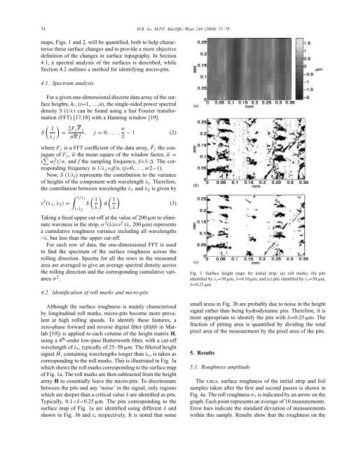The filtered height signal H ˜ , containing wavelengths longer than λr, is taken as corresponding to the roll marks. This is illustrated in Fig. 3a which shows the roll marks corresponding to the surface map of Fig. 1a. The roll marks are then subtracted from the height array H to essentially leave the micro-pits. To discriminate between the pits and any ‘noise’ in the signal, only regions which are deeper than a critical value δ are identified as pits. Typically, 0.1
Fig. 4. Roughness amplitude (r.m.s.) of strip samples. (a) Change during the pass schedule; and (b) the effect of Λs during the second pass. bottom surface of the initial strip is significantly greater than on the top surface, as observed in Fig. 1. Nevertheless, both sides of the surface have nearly conformed to the roll surface after the first pass, so that the difference between the two sides is then negligible. In the second pass, the surface roughness is further reduced slightly. The high degree to which the strip conforms to the roll surface reflects the small value of lubrication parameter Λs, which is about 0.04 for the first pass and varies between 0.015 and 0.08 for the second pass. Fig. 4b shows the effect of Λs, which is proportional to rolling speed, on the r.m.s surface roughness after the second pass. Since the surface roughness on both the incoming and outgoing strip is close to that of the rolls, any effect of Λs on surface roughness is overshadowed by scatter in the measurements. Nevertheless, there appears to be a slight increase in the surface roughness at very small Λs, which may be associated with a breakdown of lubrication. 5.2. Surface spectrum Fig. 5 shows the change in the surface spectrum during the pass schedule. The contribution of long wavelength H.R. Le, M.P.F. Sutcliffe / Wear 244 (2000) 71–78 75 Fig. 5. The change in the strip surface spectrum during rolling: (a) spectral density; and (b) cumulative surface variance, normalised by the strip roughness variance. components to the surface roughness falls through the pass schedule as these components are crushed. The increase in the high-frequency components (30–100 mm −1 ) in the first pass arises as the strip conforms to the fresh rolls used for this pass, which contain large high-frequency components. Presumably worn rolls were used to produce the initial strip surface, giving only a small high-frequency component to the ingoing strip. Although the surface roughness amplitude of the strip after the first pass approaches that of the roll surface, there is an increase in the relative composition of short wavelength components during the second pass, as the long wavelengths are crushed more readily. This is in line with the results of laboratory experiments [9] and predictions from theory [10]. Fig. 5b shows that, for the second pass, there is no significant effect of rolling speed on the surface spectra. By this pass the actual changes in roughness are slight, and any effect due to differences in hydrodynamic oil entrainment at these small values of Λs is too small to be detectable. Fig. 6 illustrates the change in surface spectrum from fresh to worn rolls. Fig. 6a plots the spectral density and
Page 1 and 2: Abstract Wear 244 (2000) 71-78 Anal
Page 3: Table 1 Details of the measurements
Page 7 and 8: Fig. 8. Pitting area of strip sampl

Analysis of surface roughness of cold-rolled aluminium foil

You also want an ePaper? Increase the reach of your titles

Delete template?

Save as template?