Digby Symons - Blade

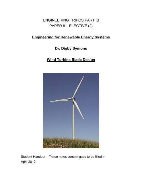
ENGINEERING TRIPOS PART IB
PAPER 8 – ELECTIVE (2)
Engineering for Renewable Energy Systems
Dr. Digby Symons
Wind Turbine Blade Design
Student Handout – These notes contain gaps to be filled in
April 2012

CONTENTS
1 Introduction ............................................................................................................. 3
2 Wind Turbine Blade Aerodynamics .................................................................. 4
2.1 Aerofoil Aerodynamics .................................................................................... 4
2.2 Wind Turbine Blade Kinematics..................................................................... 7
3 Blade Element Momentum Theory .................................................................. 12
3.1 Momentum changes ...................................................................................... 12
3.2 Blade forces .................................................................................................... 13
3.3 Induction factors ............................................................................................. 14
3.4 Iterative procedure ......................................................................................... 15
4 Optimum Performance of a Wind Turbine..................................................... 19
4.1 Turbine Power................................................................................................. 19
4.2 Optimal Induction Factors............................................................................. 19
4.3 Dependency of Power on Tip Speed Ratio................................................ 20
5 Blade Loading....................................................................................................... 21
5.1 Aerodynamic Loading.................................................................................... 21
5.2 Centrifugal Loading........................................................................................ 23
5.3 Self Weight loading ........................................................................................ 24
5.4 Combined Loading......................................................................................... 25
5.5 Storm Loading ................................................................................................ 26
More detailed coverage of the material in this handout can be found in various
books, e.g.
Aerodynamics of Wind Turbines, Hansen M.O.L. 2000
Wind Energy Explained, Manwell J.F., McGowan J.G & Rogers A.L. 2002
2

1 INTRODUCTION
1.1.1 Aim
Preliminary design of a wind turbine:
1.1.2 Wind turbine type
•
•
•
Horizontal axis wind turbine (HAWT) with 3 blade upwind rotor – the
“Danish concept”:
1.1.3 Load cases
We will consider two load cases:
Fig. 1
1) Normal operation – continuous loading
• Aerodynamic, centrifugal and self-weight loading
•
•
2) Extreme wind loading – storm loading with rotor stopped
•
3

2 WIND TURBINE BLADE AERODYNAMICS
2.1 Aerofoil Aerodynamics
2.1.1 Lift, drag and angle of attack
α
2.1.2 Lift and drag coefficients
V
c
Fig. 2
Define non-dimensional lift and drag coefficients
(1)
4

2.1.3 Variation of lift and drag coefficients with angle of attack
How does lift and drag vary with angle of attack α ?
L C C ,
D
Fig. 3
Below stall a good approximation is:
Stall:
Fig. 4
2.1.4 Application of 2D theory to wind turbines
C L
C D
• Tip leakage means flow is not purely two dimensional
• Wind turbine blades are spinning with an angular velocity ω
• The angle of attack depends on the relative wind velocity
direction.
α
(2)
5

2.1.5 Example aerofoil shape used in wind turbines
Lift and drag coefficients for the NACA 0012 symmetric aerofoil
(Miley, 1982)
CD
CL
Fig. 5
Fig. 6
6

2.2 Wind Turbine Blade Kinematics
2.2.1 Blade rotation
V
θ
ϖ r
Fig. 7
Relative
wind
Fig. 8a Fig. 8b
α
θ
7

2.2.2 Wake rotation
Axial velocity
V 0
0
Tangential velocity
0
R
V ( 1−
a)
0
Rotor
plane
Fig. 9
V ( 1−
2a)
0
8

2.2.3 Annular control volume
Wake rotates in the opposite sense to the blade rotation ω
V V ( 1−
a)
0
2.2.4 Wind and blade velocities
0
r
Fig. 10
Induced wind velocities seen by blade + blade motion
V ( 1−
a)
0
ϖ r a′
Local twist angle of blade = θ
Fig. 11
R
ϖ
V ( 1−
2a)
0
9

2.2.5 Blade relative motion and lift and drag forces
Local angle of attack = α
V ( 1−
a)
0
θ
Fig. 12
Relative wind speed Vrel has direction φ = α + θ
where sinφ = V0(
1−
a)
V rel
and cosφ = ωr(
1+
a′
)
V rel
F L and F D are aligned to the direction of
Obtain C L and C D for α = φ −θ
from table or graph for aerofoil used
Vrel
(3)
10

2.2.6 Resolve forces into normal and tangential directions
V rel
Fig. 13
We can resolve lift and drag forces into forces normal and tangential
to the rotor plane:
We can normalize these forces to obtain force coefficients:
Hence:
C N = CL
cosφ + CD
sinφ
CT = CL
sinφ − CD
cosφ
F D
F L
(4)
(5)
(6)
11

3 BLADE ELEMENT MOMENTUM THEORY
Split the blade up along its length into elements.
Use momentum theory to equate the momentum changes in the air
flowing through the turbine with the forces acting upon the blades.
Pressure distribution along curved streamlines enclosing the wake
does not give an axial force component.
(For proof see one-dimensional momentum theory, e.g. Hansen)
3.1 Momentum changes
V V ( 1−
a)
ϖ r a′
0
0
r
Fig. 14
R
ϖ
V ( 1−
2a)
Thrust from the rotor plane on the annular control volume is δ N
δ N = m&
V − u ) = 2πrρu(
V − u ) δr
( 0 1
0 1
Torque from rotor plane on this control volume is δ T
δT = m&
ru = 2m & ϖr
a′
θ
2
0
2 ϖr
a′
(7)
(8)
12

3.2 Blade forces
Now equate the momentum changes in the flow to the forces on the
blades:
3.2.1 Normal forces
2
4π
rρV a(
1 a)
δr
0 − =
2
1 V a
= Bρ 0 ( 1−
)
cCNδr
2 2
sin φ
1 ( 1−
a)
Therefore: 4 πra
= B cC
2 N
2 sin φ
Define the rotor solidity: (10)
Hence: (11)
3.2.2 Tangential forces
3 =
4π r ρV0
( 1−
a)
ωa′
δr
2
V ( 1−
a)
rω(
1+
a )
= rBρ cCTδr
2 sinφ
cosφ
1 0 ′
1 ( 1+
a′
)
Therefore: 4 πr
a′
= B cCT
2 sinφ
cosφ
(9)
(12)
Use the rotor solidity σ : (13)
13

3.3 Induction factors
These equations can be rearranged to give the axial and angular
induction factors as a function of the flow angle.
Axial induction factor:
Angular induction factor: (14)
However, recall that the flow angleφ is given by (3):
( 1−
a)
V
tanφ
=
0
( 1+
a′
) ωr
Because the flow angle φ depends on the induction factors a and a'
these equations must be solved iteratively.
14

3.4 Iterative procedure
• Choose blade aerofoil section.
• Define blade twist angle θ and chord length c as a function of
radius r.
• Define operating wind speed V0 and rotor angular velocity ω .
For a particular annular control volume of radius r :
1. Make initial choice for a and a’ , typically a = a’ = 0.
2. Calculate the flow angle φ (3).
3. Calculate the local angle of attack α = φ −θ
.
4. Find C L and C D for α from table or graph for the aerofoil used.
5. Calculate and
N
C T
C (6).
6. Calculate a and a’ (14).
7. If a and a’ have changed by more than a certain tolerance
return to step 2.
8. Calculate the local forces on the blades (7) & (8).
3.4.1 Example wind turbine
Blade element theory has been applied to an example 42 m diameter
wind turbine with the parameters below. Each element has a radial
thickness δ r = 1m.
Incident wind speed V 0
8 m/s
Angular velocity ϖ 30 rpm
Blade tip radius R 21 m
Tip speed ratio λ = ωR
/V0
Number of blades B 3
Air density ρ 1.225 kg/m 3
15

Blade shape (chord c and twist θ ) are based on the Nordtank NTK
500/41 wind turbine (see Hansen, page 62) and are plotted below
(Figs. 15 & 16).
Chord c (m)
Blade twist angle (deg)
1.8
1.6
1.4
1.2
1
0.8
0.6
0.4
0.2
0
0 2 4 6 8 10 12 14 16 18 20 22
20
18
16
14
12
10
8
6
4
2
Radius r (m)
Fig. 15: Chord c
0
0 2 4 6 8 10 12 14 16 18 20 22
r (m)
Fig. 16: Blade twist angle θ
16

3.4.2 Results of BEM analysis
Axial and angular induction factors a , a’
Induction factors a , a'
0.25
0.20
0.15
0.10
0.05
a
a'
0.00
0 2 4 6 8 10 12 14 16 18 20 22
r (m)
Fig. 17
Flow angle φ and local angle of attack α = φ −θ
Angle (deg)
30
25
20
15
10
5
0
0 2 4 6 8 10 12 14 16 18 20 22
r (m)
Fig. 18
17

Normal and tangential
N
Forces per unit length (N/m)
1100
1000
900
800
700
600
500
400
300
200
100
F T
F forces on blade
0
0 2 4 6 8 10 12 14 16 18 20 22
Total power (3 blades)
r (m)
Fig. 19
and therefore the coefficient of performance
FN (N/m)
FT (N/m)
18

4 OPTIMUM PERFORMANCE OF A WIND TURBINE
4.1 Turbine Power
The power provided by an annular control volume can be obtained
from the torque (8) as
3
2
δ P = ϖδT
= 4π
r ρV
( 1−
a)
ω a′
δr
(15)
0
The total turbine power can therefore be found by integrating over the
length R of the blades:
R
∫
2
3
P = 4πρω V ( 1−
a)
a′
r δr
(16)
0
0
We can write this expression in a non-dimensional form as:
λ
8
3
C = ( 1−
) ′
p a a x δx
(17)
∫
2
λ 0
Where λ = ωR
/V0
is the tip speed ratio and x = ωr
/V0
is the local
rotational speed ratio.
4.2 Optimal Induction Factors
For an optimally performing blade the local angle of attack will be
below stall. In this case a and a’ are not independent because,
according to potential flow theory, the total induced velocity must be
perpendicular to the local velocity (see e.g. Hansen 2000) thus
( 1−
a)
V
tanφ
=
0
( 1+
a′
) ωr
which provides the following relationship:
a′ ϖr
= (18)
aV
0
2
x a′
( 1+
a′
) = a(
1−
a)
(19)
To optimize the power we need to maximize ( 1−
a ) a′
(17) and this
requires that
1−
3a
′ =
4a
−1
a (20)
This optimal relationship between the induction factors is plotted
below in Fig. 20. As expected from the Betz limit analysis the
optimum value of a approaches 1/3.
19

1
0.9
0.8
0.7
0.6
a, a' 0.5
0.4
0.3
0.2
0.1
0
0 2 4 6 8 10
Local speed ratio x = ωr
/V0
Fig. 20: Optimal induction factors
4.3 Dependency of Power on Tip Speed Ratio
Substitution of (19) and (20) into (17) provides the dependency of the
power coefficient C p on the tip speed ratio λ (Fig. 21).
27
C
16
p
1
0.9
0.8
0.7
0.6
0.5
0.4
0.3
0.2
0.1
0
0 2 4 6 8
Tip speed ratio
λ =
ωR
V
Fig. 21: Turbine efficiency
0
a
a'
10
20

5 BLADE LOADING
5.1 Aerodynamic Loading
Once values of a and a’ have converged the blade loads can be
calculated (9) & (12):
2 2
1 V a
FN
ρ 0 ( 1−
)
=
cC
2 N
2 sin φ
F
T
1 V a ωr
a
ρ 0 ( 1−
) ( 1+
′ )
=
cC
2 sinφ
cosφ
5.1.1 Stresses at blade root
T
Fig. 22
The normal force FN
causes a “flapwise” bending moment at the root
of the blade.
M
N
=
R
∫
F
N
rmin
( r − rmin
) dr
The tangential force F T causes a tangential bending moment at the
root of the blade.
M
T
=
R
∫
F
T
rmin
( r − rmin
) dr
For convenience we will neglect the relatively small twist of the blade
cross section and assume that these bending moments are aligned
with the principal axes of the blade structural cross section. The
maximum tensile stress due to aerodynamic loading is therefore
given by:
21

5.1.2 Deflection of blade tip
dS
FN =
dr
dM
S =
dr
2
d v M
− ≈ κ =
2
dr [ EI ]( r)
Simplified approach:
• Split blade into elements.
Fig. 23
• Assume that for each element the loading FN
and flexural
rigidity EI are constant.
• Find the shear force and bending moment transferred between
each element.
• Use data book deflection coefficients for each element.
• Find the cumulative rotations along the blade.
• Find the cumulative deflections along the blade.
22

5.2 Centrifugal Loading
The large mass of a wind turbine blade and the relatively high angular
velocity can give rise to significant centrifugal stresses in the blade.
Fig. 24
Consider equilibrium of element of blade:
Simplified method:
dFc 2
= −m(
r)
ω r
dr
• Split blade up into elements.
σ c =
Fc ( r)
A(
r)
• Assume each element has a constant cross-section
Fig. 25
23

5.3 Self Weight loading
The bending moment at the blade root due to self weight loading can
dominate the stresses at the blade root. Because the turbine is
rotating the bending moment is a cyclic load with a frequency of
f = ω / 2π
. The maximum self-weight bending moment occurs when a
blade is horizontal.
Fig. 26
Bending moment at root of blade due to self weight
M
sw
=
R
∫
rmin
m(
r)
g(
r − rmin
) dr
where m(r) is the mass of the blade per unit length. This is a
tangential (edge-wise) bending moment and therefore the maximum
bending stress due to self-weight is given by:
σ
M sw b
max, sw =
I NN 2
Simplified method: split blade into elements, assume each element
has uniform self weight.
24

5.4 Combined Loading
σ
M N do
MT
b
max, aero = +
ITT
2 I NN 2
σ c =
σ
Fc ( r)
A(
r)
M sw b
max, sw
I NN 2
=
Fig. 27
Operational maximum stress: σ max = σ max, aero + σ c + σ max, sw
Minimum stress at same location: σ min = σ max, aero + σ c − σ max, sw
25

5.5 Storm Loading
5.5.1 Drag force on blade
Blades parked. Extreme wind speed
1 2
FD ( r)
ρVmaxCD
c(
r)
2
= load per unit length
V max
V max = 50 m/s, c = 1.3m
ρV c
Re = max =
μ
Hence C D =
c
F D
Fig 28
26

5.5.2 Bending moment
Find bending moment at root of blade
= ∫
R
r
M
σ
=
y
M
I
M
σ =
I
min
Ddr rF
= Eκ
do
2
3
3
i
b(
do
− d
I ≈
12
5.5.3 Shear stress
= ∫
R
r
S
min
SA y
q =
c
I
q = τtw
Note:
Ddr F
)
Fig. 29
Fig. 30
High solidity rotor (multi bladed) gives excessive forces on tower
during extreme wind speeds. Therefore use fewer blades.
27