For example what is the matrix of the linear transformation from R3 ...
For example what is the matrix of the linear transformation from R3 ...
For example what is the matrix of the linear transformation from R3 ...

Create successful ePaper yourself
Turn your PDF publications into a flip-book with our unique Google optimized e-Paper software.
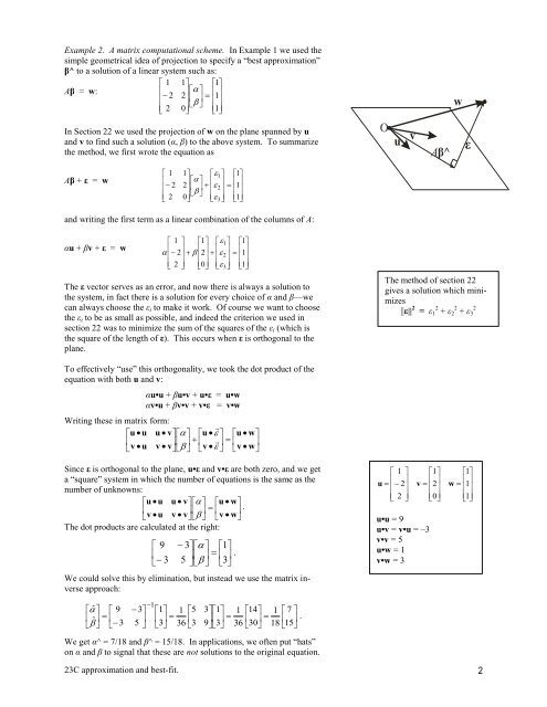
Example 2. A <strong>matrix</strong> computational scheme. In Example 1 we used <strong>the</strong><br />
simple geometrical idea <strong>of</strong> projection to specify a “best approximation”<br />
β^ to a solution <strong>of</strong> a <strong>linear</strong> system such as:<br />
1 1<br />
1<br />
Aβ = w:<br />
<br />
<br />
<br />
<br />
<br />
2 2<br />
<br />
<br />
1<br />
<br />
<br />
<br />
<br />
2 0<br />
<br />
1<br />
In Section 22 we used <strong>the</strong> projection <strong>of</strong> w on <strong>the</strong> plane spanned by u<br />
and v to find such a solution (α, β) to <strong>the</strong> above system. To summarize<br />
<strong>the</strong> method, we first wrote <strong>the</strong> equation as<br />
Aβ + ε = w<br />
1<br />
<br />
<br />
2<br />
<br />
2<br />
1<br />
1<br />
1<br />
<br />
<br />
2<br />
<br />
<br />
<br />
<br />
<br />
<br />
2<br />
<br />
1<br />
<br />
<br />
<br />
0<br />
<br />
<br />
3<br />
<br />
<br />
1<br />
and writing <strong>the</strong> first term as a <strong>linear</strong> combination <strong>of</strong> <strong>the</strong> columns <strong>of</strong> A:<br />
αu + βv + ε = w<br />
1 1<br />
1<br />
1<br />
<br />
<br />
<br />
<br />
<br />
<br />
<br />
2<br />
<br />
<br />
<br />
2<br />
<br />
2<br />
<br />
1<br />
<br />
<br />
2 <br />
<br />
0<br />
<br />
3<br />
<br />
<br />
1<br />
The ε vector serves as an error, and now <strong>the</strong>re <strong>is</strong> always a solution to<br />
<strong>the</strong> system, in fact <strong>the</strong>re <strong>is</strong> a solution for every choice <strong>of</strong> α and β––we<br />
can always choose <strong>the</strong> εi to make it work. Of course we want to choose<br />
<strong>the</strong> εi to be as small as possible, and indeed <strong>the</strong> criterion we used in<br />
section 22 was to minimize <strong>the</strong> sum <strong>of</strong> <strong>the</strong> squares <strong>of</strong> <strong>the</strong> εi (which <strong>is</strong><br />
<strong>the</strong> square <strong>of</strong> <strong>the</strong> length <strong>of</strong> ε). Th<strong>is</strong> occurs when ε <strong>is</strong> orthogonal to <strong>the</strong><br />
plane.<br />
To effectively “use” th<strong>is</strong> orthogonality, we took <strong>the</strong> dot product <strong>of</strong> <strong>the</strong><br />
equation with both u and v:<br />
αu•u + βu•v + u•ε = u•w<br />
αv•u + βv•v + v•ε = v•w<br />
Writing <strong>the</strong>se in <strong>matrix</strong> form:<br />
<br />
u<br />
u<br />
u v<br />
u<br />
<br />
u<br />
w<br />
<br />
<br />
<br />
v<br />
u<br />
v v<br />
v<br />
<br />
v<br />
w<br />
Since ε <strong>is</strong> orthogonal to <strong>the</strong> plane, u•ε and v•ε are both zero, and we get<br />
a “square” system in which <strong>the</strong> number <strong>of</strong> equations <strong>is</strong> <strong>the</strong> same as <strong>the</strong><br />
number <strong>of</strong> unknowns:<br />
u<br />
u<br />
u v<br />
u<br />
w<br />
<br />
<br />
.<br />
v<br />
u<br />
v v<br />
v<br />
w<br />
The dot products are calculated at <strong>the</strong> right:<br />
9<br />
<br />
<br />
3<br />
3<br />
1<br />
<br />
.<br />
5 <br />
3<br />
We could solve th<strong>is</strong> by elimination, but instead we use <strong>the</strong> <strong>matrix</strong> inverse<br />
approach:<br />
ˆ 9<br />
ˆ<br />
<br />
<br />
<br />
3<br />
1<br />
3<br />
1<br />
<br />
5 3<br />
1<br />
36<br />
5<br />
<br />
3<br />
31<br />
<br />
<br />
93<br />
1<br />
36<br />
14<br />
<br />
30<br />
1<br />
18<br />
7 <br />
.<br />
15<br />
We get α^ = 7/18 and β^ = 15/18. In applications, we <strong>of</strong>ten put “hats”<br />
on α and β to signal that <strong>the</strong>se are not solutions to <strong>the</strong> original equation.<br />
23C approximation and best-fit. 2<br />
O<br />
u v<br />
1 <br />
u <br />
<br />
<br />
2<br />
<br />
<br />
2 <br />
Aβ^<br />
1<br />
v <br />
<br />
<br />
2<br />
<br />
<br />
0<br />
w<br />
ε<br />
The method <strong>of</strong> section 22<br />
gives a solution which minimizes<br />
||ε|| 2 = ε1 2 + ε2 2 + ε3 2<br />
u•u = 9<br />
u•v = v•u = –3<br />
v•v = 5<br />
u•w = 1<br />
v•w = 3<br />
1<br />
w <br />
<br />
<br />
1<br />
<br />
<br />
1