For example what is the matrix of the linear transformation from R3 ...

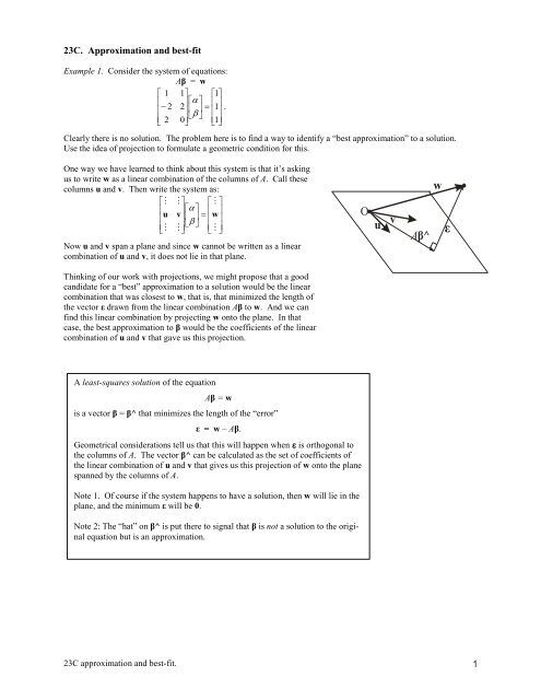
23C. Approximation and best-fit
Example 1. Consider the system of equations:
Aβ = w
1 1
1
2 2
1
.
2 0
1
Clearly there is no solution. The problem here is to find a way to identify a “best approximation” to a solution.
Use the idea of projection to formulate a geometric condition for this.
One way we have learned to think about this system is that it’s asking
us to write w as a linear combination of the columns of A. Call these
columns u and v. Then write the system as:
u v
w
Now u and v span a plane and since w cannot be written as a linear
combination of u and v, it does not lie in that plane.
Thinking of our work with projections, we might propose that a good
candidate for a “best” approximation to a solution would be the linear
combination that was closest to w, that is, that minimized the length of
the vector ε drawn from the linear combination Aβ to w. And we can
find this linear combination by projecting w onto the plane. In that
case, the best approximation to β would be the coefficients of the linear
combination of u and v that gave us this projection.
A least-squares solution of the equation
Aβ = w
is a vector β = β^ that minimizes the length of the “error”
ε = w – Aβ.
Geometrical considerations tell us that this will happen when is orthogonal to
the columns of A. The vector β^ can be calculated as the set of coefficients of
the linear combination of u and v that gives us this projection of w onto the plane
spanned by the columns of A.
Note 1. Of course if the system happens to have a solution, then w will lie in the
plane, and the minimum ε will be 0.
Note 2: The “hat” on β^ is put there to signal that β is not a solution to the original
equation but is an approximation.
23C approximation and best-fit. 1
O
u v
Aβ^
w
ε

Example 2. A matrix computational scheme. In Example 1 we used the
simple geometrical idea of projection to specify a “best approximation”
β^ to a solution of a linear system such as:
1 1
1
Aβ = w:
2 2
1
2 0
1
In Section 22 we used the projection of w on the plane spanned by u
and v to find such a solution (α, β) to the above system. To summarize
the method, we first wrote the equation as
Aβ + ε = w
1
2
2
1
1
1
2
2
1
0
3
1
and writing the first term as a linear combination of the columns of A:
αu + βv + ε = w
1 1
1
1
2
2
2
1
2
0
3
1
The ε vector serves as an error, and now there is always a solution to
the system, in fact there is a solution for every choice of α and β––we
can always choose the εi to make it work. Of course we want to choose
the εi to be as small as possible, and indeed the criterion we used in
section 22 was to minimize the sum of the squares of the εi (which is
the square of the length of ε). This occurs when ε is orthogonal to the
plane.
To effectively “use” this orthogonality, we took the dot product of the
equation with both u and v:
αu•u + βu•v + u•ε = u•w
αv•u + βv•v + v•ε = v•w
Writing these in matrix form:
u
u
u v
u
u
w
v
u
v v
v
v
w
Since ε is orthogonal to the plane, u•ε and v•ε are both zero, and we get
a “square” system in which the number of equations is the same as the
number of unknowns:
u
u
u v
u
w
.
v
u
v v
v
w
The dot products are calculated at the right:
9
3
3
1
.
5
3
We could solve this by elimination, but instead we use the matrix inverse
approach:
ˆ 9
ˆ
3
1
3
1
5 3
1
36
5
3
31
93
1
36
14
30
1
18
7
.
15
We get α^ = 7/18 and β^ = 15/18. In applications, we often put “hats”
on α and β to signal that these are not solutions to the original equation.
23C approximation and best-fit. 2
O
u v
1
u
2
2
Aβ^
1
v
2
0
w
ε
The method of section 22
gives a solution which minimizes
||ε|| 2 = ε1 2 + ε2 2 + ε3 2
u•u = 9
u•v = v•u = –3
v•v = 5
u•w = 1
v•w = 3
1
w
1
1

As a check we calculate the error:
= w – Aβ^ =
1
1 1
1
11
1
–
1 7
2 2
=
1
18
1
2 0
15
1
–
8
=
9
1
7
2
1
1
9
2
and check that it is orthogonal to the vectors u and v. Always do that!
A technical note:
In text-books on the subject, you will often see the original equation
1 1
1
1
Aβ + ε = w
2 2
2
1
2 0
3
1
transformed by multiplying both sides on the left by the transpose of A.
A T Aβ + A T = A T 1 1
1
1
w 1 2 2
1 2 2
1 2 2
2 2
2
1
1
2 0
1
2 0
1
2 0
2 0
3
1
This is actually just a wonderfully slick way of getting our 2×2 system.
For example consider the product of the first two matrices. The first is
2×3 and the second is 3×2 and the product will then be 2×2. Now if
you think carefully about the terms of the matrix products, you will see
that they are dot products. Thus, the entries of the matrix A T A are the
dot products u•u, u•v, v•u and v•v and the system above is simply:
(A T A)β + A T = A T w
u
u
v
u
u v
u
u
w
v v
v
v
w
No matter how you think of it, what is important is that you can easily arrive at the corresponding square system of
equations which will allow you to find the least-squares approximation. The forms of these matrices are given below
for the 2×2 and the 3×3 cases.
Table of matrices for the 2×2 and 3×3 cases
u
u
u
u v
A = [u v] A T A =
u
v
v
v
u v v
A = [u v w]
u
w
The least-squares solution of the equation
A T A = v u v w
u
u
v u
w u
Aβ = w
is the solution β = β^ of the “square” system of equations:
A T Aβ = A T w.
w v
u w
v w
w w
A T w =
u
u
w
w
v
v
w
23C approximation and best-fit. 3
u v
v v
A T z =
O
u v
Here A T is the transpose of A,
defined as the matrix whose
rows are the columns of A.
Thus:
1
2
2
1
2
0
T
Aβ^
u
u
z
v
z
v z
w
w z
w
ε
1 2
1
2
2
.
0

Example 3. Find the least squares approximation to the solution of the
system of equations:
2x + y = 3
x – y = 1
x + y = 2
Soln.
In matrix form the system is:
2
1
1
Ax = b
1 3
x
1
1
.
y
1
2
The equation for the least-squares solution x is A T Ax = A T b.
We calculate:
A T
u
u
A
v
u
u v
6
v v
2
And the equation to be solved is:
The solution is:
^
x
6
y
2
6
2
1
2
9
3
4
We get: x^ = 19/14, y^ = 6/14.
2
3
T
A w
2
x
9
3
y
4
1 3
14
2
u
w
9
4
v
w
29
6 4
1 19
.
14 6
Example 4. Use the above approach to find a least squares solution for
the equation
1 6
3
0 5
1
.
2
3
2
Solution. The new system is:
1
6
0
5
1 2
0
3
2
6
1
5
6
3
0
5
5
0
0
7
70
17
3
2
1
3
2
The equations are uncoupled, the first involving only α and the second
only β. They read 5α = 7 and 70β = –17 and the solution is
ˆ 7 / 5
ˆ
.
17
/ 70
2
u
1
1
u•u = 6
u•v = v•u = 2
v•v = 3
u•w = 9
v•w = 4
1
v
1
1
3
w
1
2
Note: This is an example in which
the columns of A are orthogonal.
Notice that this gives us a diagonal
coefficient matrix for our new system,
and the solution can be found
immediately.
23C approximation and best-fit. 4

Example 5. Find the line y = x + that “best fits” the data at the
right and calculate and display the error vector defined as the difference
between the y-value of the point and the height of the approximating
line. [Thus in the diagram, ε2 is positive (point above the line) and
the other three errors are negative..
Solution. Plug the data points into the equation. We get:
yi = xi + + εi
10 = α + β + ε1
40 = 2α + β + ε2
20 = 3α + β + ε3
30 = 4α + β + ε4
where the εi are the "errors" which measure the vertical distance between
the ith data point and the line. In vector-matrix form, this is
1
2
3
4
X + = y.
1
1
10
1
2
40
.
1
3 20
1
4 30
If there was a line passing exactly through all four data points then we
could find a pair (α, β) which satisfied all four equation with εi = 0. But
this is not the case so we try to choose α and β to make the error as small
as possible. The ideas above tell us that this will be the case when is
orthogonal to the columns of the matrix X. In this example, these are vectors
in R 4 , but the same dot product analysis works. The system we get is:
^
30
^
10
u
u
v
u
10
4
30
10
1
u v
u
w
v v
v
w
10
270
4
100
270
100
1
20
4
10
10270
4
30
100
15
This tells us that the best fit line is y = 4x + 15. The error is:
=
1
2
3
4
= y – X^ =
10
1
40
2
20
3
30
4
As usual, check that is orthogonal to the columns of X.
1
9
1
4
17
.
115
7
1
1
23C approximation and best-fit. 5
50
y
40
30
20
10
0 1
x y
1 10
2 40
3 20
4 30
1
2
3
4
x
2 3 4 5
The εi are actually signed errors: when
the point is below the line, εi is negative.
This is clear from the equations
at the right.
1
1
2
1
u v
3
1
4
1
u•u = 30
u•v = v•u = 10
v•v = 4
u•y = 270
v•y = 100
10
40
y
20
30
The regression line is often
called the least squares line.
That’s because it is the sum of
the squares of the errors i that
is being minimized.

Example 6. The data points at the right have been observed.
It is desired to fit a quadratic regression model:
y = x 2 + x + .
Find the least squares quadratic polynomial and plot its graph
along with the data points. Calculate the residual vector .
Solution: We write the six equations, one for each data point as
the vector equation:
0
0
1
1
4
4
0
0
1
1
2
2
X + = y.
1
1
0
1
2
1
1
3 0
1
4 1
1
1
5
1
6
2
The condition that be orthogonal to the columns of X is:
34
18
10
X T = 0
X T (y – X) = 0
X T X = X T y
18
10
6
10
13
6
7 .
6
5
We can solve this by solving the system of equations by elimination
or using technology to calculate the matrix inverse. A good website
is: http://www.bluebit.gr/matrix-calculator/calculate.aspx
The solution is
^
34
^
18
^
10
18
10
6
10
6
6
1
giving us the best fit parabola
The residual vector is
= y – X^ =
13
3
1
7
6
4
5
1
1 2
y = (x – x + 1) .
2
0
0
1
0
0
1
1
1
1
4
2
4
0
0
1
1
2
2
6
13
3
1
1
1
1
1
1
1 1 1
1
1
2 2
1
1
1
1
1
1
As usual, check that is orthogonal to the columns of X .
1 13
1
1
3
7
1
2
2
5
1
x y
0 0
0 1
1 0
1 1
2 1
2 2
23C approximation and best-fit. 6
3
2
1
0
3
2
1
0
y
y
0 1 2 3
0
0
0
0
1
1
u v
1
1
4
2
4
2
u•u = 34
v•v = 10
w•w = 6
u•v = v•u = 18
u•w = w•u = 10
v•w = w•v = 6
1
1
1
w
1
1
1
y= (x^ 2 - x + 1)/2
0 1 2 3
x
x
0
1
0
y
1
1
2
Having seen this picture, can
you see a way you might have
deduced that this would have to
be the answer without doing
any work at all?

Example 7. Find the plane z = x + y that “best fits” the data at the
right and calculate and display the error vector .
Solution. Plug the data points into the equation. We get:
zi = xi + yi
10 = α + β + ε1
30 = α + 2β + ε2
20 = 2α + β + ε3
50 = 2α + 2β + ε4
where the εi are the "errors" which measure the vertical distance between
the ith data point and the plane. In vector-matrix form, this is
1
1
2
2
X + = z.
1
1
10
2
2
30
.
1
3 20
2
4 50
The least-squares condition is that ε be orthogonal to the columns of the
matrix X, that is X T ε = 0. And the algebraic condition for that is:
^
10
^
9
9
10
x
x
y
x
1
10
9
(X T X) = X T y
180
190
This tells us that the best fit plane is
The error is:
=
1
2
3
4
= z–X^ =
x y
x
z
y y
y
z
9
180
10
190
1
19
10
9
9180
10 190
1
z ( 90x
280y)
.
19
10
30
1
20
19
50
1
1
2
2
1
2
90
1280
2
As usual, check that is orthogonal to the columns of X.
1
19
1
19
90
280
190
370
570 650
380
460
950
740
180
80
.
80
210
23C approximation and best-fit. 7
1
19
x
x y z
1 1 10
1 2 30
2 1 20
2 2 50
z
1
1
1
2
x y
2
1
2
2
x•x = 10
x•y = y•x = 9
y•y = 10
x•z = 180
y•z = 190
10
30
z
20
50
y

Example 8. At the right is tabulated the mid-term test mark (out of
10) and the final marks for four of Jason’s friends who took the course
last year. Jason’s mid-year test mark is 7. He decides to use a linear
model
y = mx + b
to predict his final mark. What does he discover?
Solution.
We use a “least squares” model. The equations are:
90 = 8m + b
85 = 7m + b
95 = 9m + b
75 = 7m + b
In matrix form:
8
7
9
7
Xb = y
1
90
1
m
85
.
1
b
95
1
75
The least squares solution b^ is the solution of the equation:
243
31
m^
243
b^
31
The best fit recursive equation is
(X T X)b^ = X T y.
31m^
2695
4
b^
345
31
4
1
2695
345
y = (85x + 290)/11
1 85
.
11 290
Jason’s estimate of his final mark is y = (85×7 + 290)/11 = 80.4.
student Mid Final
Brenda 8 90
Alnoor 7 87
Kit 9 94
Tim 7 75
23C approximation and best-fit. 8