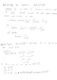
For example what is the matrix of the linear transformation from R3 ...

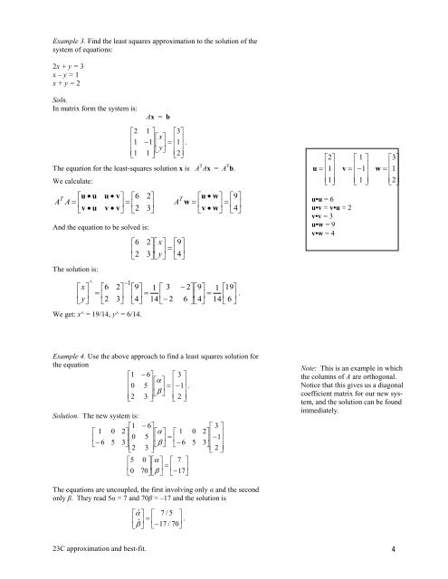
Example 3. Find the least squares approximation to the solution of the
system of equations:
2x + y = 3
x – y = 1
x + y = 2
Soln.
In matrix form the system is:
2
1
1
Ax = b
1 3
x
1
1
.
y
1
2
The equation for the least-squares solution x is A T Ax = A T b.
We calculate:
A T
u
u
A
v
u
u v
6
v v
2
And the equation to be solved is:
The solution is:
^
x
6
y
2
6
2
1
2
9
3
4
We get: x^ = 19/14, y^ = 6/14.
2
3
T
A w
2
x
9
3
y
4
1 3
14
2
u
w
9
4
v
w
29
6 4
1 19
.
14 6
Example 4. Use the above approach to find a least squares solution for
the equation
1 6
3
0 5
1
.
2
3
2
Solution. The new system is:
1
6
0
5
1 2
0
3
2
6
1
5
6
3
0
5
5
0
0
7
70
17
3
2
1
3
2
The equations are uncoupled, the first involving only α and the second
only β. They read 5α = 7 and 70β = –17 and the solution is
ˆ 7 / 5
ˆ
.
17
/ 70
2
u
1
1
u•u = 6
u•v = v•u = 2
v•v = 3
u•w = 9
v•w = 4
1
v
1
1
3
w
1
2
Note: This is an example in which
the columns of A are orthogonal.
Notice that this gives us a diagonal
coefficient matrix for our new system,
and the solution can be found
immediately.
23C approximation and best-fit. 4