The Kernel and Range of a Linear Transformation

360 CHAPTER 5 Linear Transformations
For Problems 5–12, describe the transformation of R2 with
the given matrix as a product of reflections, stretches, and
shears.
12
5. A = .
01
6. A =
7. A =
8. A =
9. A =
02
.
20
10
.
31
−1 0
.
0 −1
1 −3
.
−2 8
12
10. A = .
34
1 0
11. A = .
0 −2
−1 −1
12. A = .
−1 0
13. Consider the transformation of R 2 corresponding to a
counterclockwise rotation through angle θ (0 ≤ θ<
2π). For θ = π/2, 3π/2, verify that the matrix of the
transformation is given by (5.2.5), and describe it in
terms of reflections, stretches, and shears.
14. Express the transformation of R 2 corresponding to a
counterclockwise rotation through an angle θ = π/2
as a product of reflections, stretches, and shears. Repeat
for the case θ = 3π/2.
5.3 The Kernel and Range of a Linear Transformation
If T : V → W is any linear transformation, there is an associated homogeneous linear
vector equation, namely,
T(v) = 0.
The solution set to this vector equation is a subset of V called the kernel of T .
DEFINITION 5.3.1
Let T : V → W be a linear transformation. The set of all vectors v ∈ V such that
T(v) = 0 is called the kernel of T and is denoted Ker(T ). Thus,
Ker(T ) ={v ∈ V : T(v) = 0}.
Example 5.3.2 Determine Ker(T ) for the linear transformation T : C 2 (I) → C 0 (I) defined by T(y)=
y ′′ + y.
Solution: We have
Ker(T ) ={y ∈ C 2 (I) : T(y)= 0} ={y ∈ C 2 (I) : y ′′ + y = 0 for all x ∈ I}.
Hence, in this case, Ker(T ) is the solution set to the differential equation
y ′′ + y = 0.
Since this differential equation has general solution y(x) = c1 cos x + c2 sin x,wehave
Ker(T ) ={y ∈ C 2 (I) : y(x) = c1 cos x + c2 sin x}.
This is the subspace of C 2 (I) spanned by {cos x,sin x}.
The set of all vectors in W that we map onto when T is applied to all vectors in V is
called the range of T . We can think of the range of T as being the set of function output
values. A formal definition follows.

5.3 The Kernel and Range of a Linear Transformation 361
DEFINITION 5.3.3
The range of the linear transformation T : V → W is the subset of W consisting of
all transformed vectors from V . We denote the range of T by Rng(T ). Thus,
Rng(T ) ={T(v) : v ∈ V }.
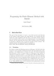
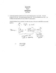
A schematic representation of Ker(T ) and Rng(T ) is given in Figure 5.3.1.
Ker(T)
0
Every vector in Ker(T) is mapped
to the zero vector in W
V
Rng(T)
Figure 5.3.1: Schematic representation of the kernel and range of a linear transformation.
Let us now focus on matrix transformations, say T : Rn → Rm . In this particular
case,
Ker(T ) ={x ∈ R n : T(x) = 0}.
If we let A denote the matrix of T , then T(x) = Ax, so that
Consequently,
Ker(T ) ={x ∈ R n : Ax = 0}.
If T : R n → R m is the linear transformation with matrix A, then Ker(T ) is
the solution set to the homogeneous linear system Ax = 0.
In Section 4.3, we defined the solution set to Ax = 0 to be nullspace(A). Therefore, we
have
Ker(T ) = nullspace(A), (5.3.1)
from which it follows directly that 2 Ker(T ) is a subspace of R n . Furthermore, for a linear
transformation T : R n → R m ,
Rng(T ) ={T(x) : x ∈ R n }.
If A =[a1, a2,...,an] denotes the matrix of T , then
Rng(T ) ={Ax : x ∈ R n }
={x1a1 + x2a2 +···+xnan : x1,x2,...,xn ∈ R}
= colspace(A).
Consequently, Rng(T ) is a subspace of R m . We illustrate these results with an example.
Example 5.3.4 Let T : R 3 → R 2 be the linear transformation with matrix
A =
1 −2 5
.
−2 4 −10
2 It is also easy to verify this fact directly by using Definition 5.3.1 and Theorem 4.3.2.
0
W

362 CHAPTER 5 Linear Transformations
Determine Ker(T ) and Rng(T ).
Solution: To determine Ker(T ), (5.3.1) implies that we need to find the solution set
to the system Ax = 0. The reduced row-echelon form of the augmented matrix of this
system is
1 −2 50
,
0 000
so that there are two free variables. Setting x2 = r and x3 = s, it follows that x1 = 2r−5s,
so that x = (2r − 5s, r, s). Hence,
Ker(T ) ={x ∈ R 3 : x = (2r − 5s, r, s): r, s ∈ R}
={x ∈ R 3 : x = r(2, 1, 0) + s(−5, 0, 1), r, s ∈ R}.
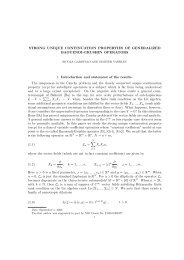
We see that Ker(T ) is the two-dimensional subspace of R 3 spanned by the linearly
independent vectors (2, 1, 0) and (−5, 0, 1), and therefore it consists of all points lying
on the plane through the origin that contains these vectors. We leave it as an exercise to
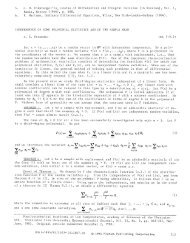
verify that the equation of this plane is x1 − 2x2 + 5x3 = 0. The linear transformation
T maps all points lying on this plane to the zero vector in R 2 . (See Figure 5.3.2.)
x 1
x 3
x 1 2x 2 5x 3 0
Ker(T)
x
x 2
y 2 2y 1
y 2
Rng(T)
T(x)
Figure 5.3.2: The kernel and range of the linear transformation in Example 5.3.6.
Turning our attention to Rng(T ), recall that, since T is a matrix transformation,
Rng(T ) = colspace(A).
From the foregoing reduced row-echelon form of A we see that colspace(A) is generated
by the first column vector in A. Consequently,
Rng(T ) ={y ∈ R 2 : y = r(1, −2), r ∈ R}.
Hence, the points in Rng(T ) lie along the line through the origin in R2 whose direction
is determined by v = (1, −2). The Cartesian equation of this line is y2 = −2y1.
Consequently, T maps all points in R3 onto this line, and therefore Rng(T ) is a onedimensional
subspace of R2 . This is illustrated in Figure 5.3.2.
To summarize, any matrix transformation T : Rn → Rm with m × n matrix A has
natural subspaces
Ker(T ) = nullspace(A) (subspace of R n )
Rng(T ) = colspace(A) (subspace of R m )
Now let us return to arbitrary linear transformations. The preceding discussion has
shown that both the kernel and range of any linear transformation from R n to R m are
y 1

5.3 The Kernel and Range of a Linear Transformation 363
subspaces of R n and R m , respectively. Our next result, which is fundamental, establishes
that this is true in general.
Theorem 5.3.5 If T : V → W is a linear transformation, then
1. Ker(T ) is a subspace of V .
2. Rng(T ) is a subspace of W.
Proof In this proof, we once more denote the zero vector in W by 0W . Both Ker(T )
and Rng(T ) are necessarily nonempty, since, as we verified in Section 5.1, any linear
transformation maps the zero vector in V to the zero vector in W. We must now establish
that Ker(T ) and Rng(T ) are both closed under addition and closed under scalar
multiplication in the appropriate vector space.
1. If v1 and v2 are in Ker(T ), then T(v1) = 0W and T(v2) = 0W . We must show
that v1 + v2 is in Ker(T ); that is, T(v1 + v2) = 0W . But we have
T(v1 + v2) = T(v1) + T(v2) = 0W + 0W = 0W ,
so that Ker(T ) is closed under addition. Further, if c is any scalar,
T(cv1) = cT (v1) = c0W = 0W ,
which shows that cv1 is in Ker(T ), and so Ker(T ) is also closed under scalar
multiplication. Thus, Ker(T ) is a subspace of V .
2. If w1 and w2 are in Rng(T ), then w1 = T(v1) and w2 = T(v2) for some v1 and
v2 in V . Thus,
w1 + w2 = T(v1) + T(v2) = T(v1 + v2).
This says that w1 +w2 arises as an output of the transformation T ; that is, w1 +w2
is in Rng(T ). Thus, Rng(T ) is closed under addition. Further, if c is any scalar,
then
cw1 = cT (v1) = T(cv1),
so that cw1 is the transform of cv1, and therefore cw1 is in Rng(T ). Consequently,
Rng(T ) is a subspace of W.
Remark We can interpret the first part of the preceding theorem as telling us that if T
is a linear transformation, then the solution set to the corresponding linear homogeneous
problem
T(v) = 0
is a vector space. Consequently, if we can determine the dimension of this vector space,
then we know how many linearly independent solutions are required to build every
solution to the problem. This is the formulation for linear problems that we have been
looking for.
Example 5.3.6 Find Ker(S), Rng(S), and their dimensions for the linear transformation S : M2(R) →
M2(R) defined by
S(A) = A − A T .

364 CHAPTER 5 Linear Transformations
Solution: In this case,
Ker(S) ={A ∈ M2(R): S(A) = 0} ={A ∈ M2(R): A − A T = 02}.
Thus, Ker(S) is the solution set of the matrix equation
so that the matrices in Ker(S) satisfy
A − A T = 02,
A T = A.
Hence, Ker(S) is the subspace of M2(R) consisting of all symmetric 2 × 2 matrices. We
have shown previously that a basis for this subspace is
10
,
00
01
,
10
00
,
01
so that dim[Ker(S)] = 3. We now determine the range of S:
Rng(S) ={S(A): A ∈ M2(R)} ={A− A T : A ∈ M2(R)}
ab a c
= − : a, b, c, d ∈ R
cd bd
0 b − c
=
: b, c ∈ R .
−(b − c) 0
Thus,
0 e
01
Rng(S) = : e ∈ R = span .
−e 0
−1 0
Consequently, Rng(S) consists of all skew-symmetric 2 ×2 matrices with real elements.
Since Rng(S) is generated by the single nonzero matrix
01
,
−1 0
it follows that a basis for Rng(S) is
01
,
−1 0
so that dim[Rng(S)] = 1.
Example 5.3.7 Let T : P1 → P2 be the linear transformation defined by
T(a+ bx) = (2a − 3b) + (b − 5a)x + (a + b)x 2 .
Find Ker(T ), Rng(T ), and their dimensions.
Solution: From Definition 5.3.1,
Ker(T ) ={p ∈ P1 : T(p)= 0}
={a + bx : (2a − 3b) + (b − 5a)x + (a + b)x 2 = 0 for all x}
={a + bx : a + b = 0, b− 5a = 0, 2a − 3b = 0}.

5.3 The Kernel and Range of a Linear Transformation 365
But the only values of a and b that satisfy the conditions
a + b = 0, b− 5a = 0, 2a − 3b = 0
are
a = b = 0.
Consequently, Ker(T ) contains only the zero polynomial. Hence, we write
Ker(T ) ={0}.
It follows from Definition 4.6.7 that dim[Ker(T )] = 0. Furthermore,
Rng(T ) ={T(a+ bx): a,b ∈ R} ={(2a − 3b) + (b − 5a)x + (a + b)x 2 : a,b ∈ R}.
To determine a basis for Rng(T ), we write this as
Rng(T ) ={a(2 − 5x + x 2 ) + b(−3 + x + x 2 ) : a,b ∈ R}
= span{2 − 5x + x 2 , −3 + x + x 2 }.
Thus, Rng(T ) is spanned by p1(x) = 2 − 5x + x 2 and p2(x) =−3 + x + x 2 . Since
p1 and p2 are not proportional to one another, they are linearly independent on any
interval. Consequently, a basis for Rng(T ) is {2 − 5x + x 2 , −3 + x + x 2 }, so that
dim[Rng(T )] = 2.
The General Rank-Nullity Theorem
In concluding this section, we consider a fundamental theorem for linear transformations
T : V → W that gives a relationship between the dimensions of Ker(T ), Rng(T ), and
V . This is a generalization of the Rank-Nullity Theorem considered in Section 4.9. The
theorem here, Theorem 5.3.8, reduces to the previous result, Theorem 4.9.1, in the case
when T is a linear transformation from R n to R m with m × n matrix A. Suppose that
dim[V ]=n and that dim[Ker(T )] = k. Then k-dimensions worth of the vectors in V
are all mapped onto the zero vector in W. Consequently, we only have n − k dimensions
worth of vectors left to map onto the remaining vectors in W. This suggests that
dim[Rng(T )] = dim[V ]−dim[Ker(T )].
This is indeed correct, although a rigorous proof is somewhat involved. We state the
result as a theorem here.
Theorem 5.3.8 (General Rank-Nullity Theorem)
If T : V → W is a linear transformation and V is finite-dimensional, then
dim[Ker(T )]+dim[Rng(T )] =dim[V ].
Before presenting the proof of this theorem, we give a few applications and examples.
The general Rank-Nullity Theorem is useful for checking that we have the correct
dimensions when determining the kernel and range of a linear transformation. Furthermore,
it can also be used to determine the dimension of Rng(T ), once we know the
dimension of Ker(T ), or vice versa. For example, consider the linear transformation
discussed in Example 5.3.6. Theorem 5.3.8 tells us that
dim[Ker(S)] + dim[Rng(S)] = dim[M2(R)],

366 CHAPTER 5 Linear Transformations
so that once we have determined that dim[Ker(S)] = 3, it immediately follows that
so that
3 + dim[Rng(S)] =4
dim[Rng(S)] =1.
As another illustration, consider the matrix transformation in Example 5.3.4 with
A =
1 −2 5
−2 4 −10
By inspection, we can see that dim[Rng(T )] = dim[colspace(A)] = 1, so the Rank-
Nullity Theorem implies that
.
dim[Ker(T )] = 3 − 1 = 2,
with no additional calculation. Of course, to obtain a basis for Ker(T ), it becomes
necessary to carry out the calculations presented in Example 5.3.4.
We close this section with a proof of Theorem 5.3.8.
Proof of Theorem 5.3.8: Suppose that dim[V ]=n. We consider three cases:
Case 1: If dim[Ker(T )] = n, then by Corollary 4.6.14 we conclude that Ker(T ) = V .
This means that T(v) = 0 for every vector v ∈ V . In this case
hence dim[Rng(T )] = 0. Thus, we have
as required.
Rng(T ) ={T(v): v ∈ V }={0},
dim[Ker(T )]+dim[Rng(T )] =n + 0 = n = dim[V ],
Case 2: Assume dim[Ker(T )] = k, where 0

Exercises for 5.3
Key Terms
5.3 The Kernel and Range of a Linear Transformation 367
where dk+1,dk+2,...,dn are scalars. Then, using the linearity of T ,
T(dk+1vk+1 + dk+2vk+2 +···+dnvn) = 0,
which implies that the vector dk+1vk+1 + dk+2vk+2 +···+dnvn is in Ker(T ). Consequently,
there exist scalars d1,d2,...,dk such that
which means that
dk+1vk+1 + dk+2vk+2 +···+dnvn = d1v1 + d2v2 +···+dkvk,
d1v1 + d2v2 +···+dkvk − (dk+1vk+1 + dk+2vk+2 +···+dnvn) = 0.
Since the set of vectors {v1, v2,...,vk, vk+1,...,vn} is linearly independent, we must
have
d1 = d2 =···=dk = dk+1 =···=dn = 0.
Thus, from Equation (5.3.2), {T(vk+1), T (vk+2),...,T(vn)} is linearly independent.
By the work in the last two paragraphs, {T(vk+1), T (vk+2),...,T(vn)} is a basis
for Rng(T ). Since there are n − k vectors in this basis, it follows that dim[Rng(T )]
= n − k. Consequently,
as required.
Kernel and range of a linear transformation, Rank-Nullity
Theorem.
Skills
• Be able to find the kernel of a linear transformation
T : V → W and give a basis and the dimension of
Ker(T ).
• Be able to find the range of a linear transformation
T : V → W and give a basis and the dimension of
Rng(T ).
• Be able to show that the kernel (resp. range) of a linear
transformation T : V → W is a subspace of V (resp.
W).
• Be able to verify the Rank-Nullity Theorem for a given
linear transformation T : V → W.
dim[Ker(T )]+dim[Rng(T )] =k + (n − k) = n = dim[V ],
Case 3: If dim[Ker(T )] = 0, then Ker(T ) ={0}. Let {v1, v2,...,vn} be any basis
for V . By a similar argument to that used in Case 2 above, it can be shown that (see
Problem 18) {T(v1), T (v2),...,T(vn)} is a basis for Rng(T ), and so again we have
dim[Ker(T )]+dim[Rng(T )] =n.
• Be able to utilize the Rank-Nullity Theorem to help
find the dimensions of the kernel and range of a linear
transformation T : V → W.
True-False Review
For Questions 1–6, decide if the given statement is true or
false, and give a brief justification for your answer. If true,
you can quote a relevant definition or theorem from the text.
If false, provide an example, illustration, or brief explanation
of why the statement is false.
1. If T : V → W is a linear transformation and W is
finite-dimensional, then
dim[Ker(T )]+dim[Rng(T )] =dim[W].
2. If T : P4 → R 7 is a linear transformation, then Ker(T )
must be at least two-dimensional.

368 CHAPTER 5 Linear Transformations
3. If T : R n → R m is a linear transformation with matrix
A, then Rng(T ) is the solution set to the homogeneous
linear system Ax = 0.
4. The range of a linear transformation T : V → W is a
subspace of V .
5. If T : M23 → P7 is a linear transformation with
111
123
T = 0, T = 0,
000
456
then Rng(T ) is at most four-dimensional.
6. If T : R n → R m is a linear transformation with matrix
A, then Rng(T ) is the column space of A.
Problems
1. Consider T : R3 → R2 defined by T(x) = Ax, where
1 −1 2
A
.
1 −2 −3
Find T(x) and thereby determine whether x is in
Ker(T ).
(a) x = (7, 5, −1).
(b) x = (−21, −15, 2).
(c) x = (35, 25, −5).
For Problems 2–6, find Ker(T ) and Rng(T ) and give a geometrical
description of each. Also, find dim[Ker(T )] and
dim[Rng(T )] and verify Theorem 5.3.8.
2. T : R 2 → R 2 defined by T(x) = Ax, where
A =
36
12
.
3. T : R3 → R3 defined by T(x) = Ax, where
⎡ ⎤
1 −1 0
A = ⎣ 0 1 2⎦
.
2 −1 1
4. T : R3 → R3 defined by T(x) = Ax, where
⎡ ⎤
1 −2 1
A = ⎣ 2 −3 −1 ⎦ .
5 −8 −1
5. T : R3 → R2 defined by T(x) = Ax, where
1 −1 2
A =
.
−3 3 −6
6. T : R 3 → R 2 defined by T(x) = Ax, where
A =
132
265
.
For Problems 7–10, compute Ker(T ) and Rng(T ).
7. The linear transformation T defined in Problem 24 in
Section 5.1.
8. The linear transformation T defined in Problem 25 in
Section 5.1.
9. The linear transformation T defined in Problem 26 in
Section 5.1.
10. The linear transformation T defined in Problem 27 in
Section 5.1.
11. Consider the linear transformation T : R3 → R defined
by
T(v) =〈u, v〉,
where u is a fixed nonzero vector in R3 .
(a) Find Ker(T ) and dim[Ker(T )], and interpret this
geometrically.
(b) Find Rng(T ) and dim[Rng(T )].
12. Consider the linear transformation S : Mn(R) →
Mn(R) defined by S(A) = A + A T , where A is a
fixed n × n matrix.
(a) Find Ker(S) and describe it. What is
dim[Ker(S)]?
(b) In the particular case when A isa2× 2 matrix,
determine a basis for Ker(S), and hence, find its
dimension.
13. Consider the linear transformation T : Mn(R) →
Mn(R) defined by
T (A) = AB − BA,
where B isafixedn × n matrix. Find Ker(T ) and
describe it.
14. Consider the linear transformation T : P2 → P2 defined
by
T(ax 2 +bx+c) = ax 2 +(a+2b+c)x+(3a−2b−c),
where a,b, and c are arbitrary constants.
(a) Show that Ker(T ) consists of all polynomials of
the form b(x − 2), and hence, find its dimension.
(b) Find Rng(T ) and its dimension.

15. Consider the linear transformation T : P2 → P1 defined
by
T(ax 2 + bx + c) = (a + b) + (b − c)x,
where a,b, and c are arbitrary real numbers. Determine
Ker(T ), Rng(T ), and their dimensions.
16. Consider the linear transformation T : P1 → P2 defined
by
T(ax+ b) = (b − a) + (2b − 3a)x + bx 2 .
Determine Ker(T ), Rng(T ), and their dimensions.
17. Let {v1, v2, v3} and {w1, w2} be bases for real vector
spaces V and W, respectively, and let T : V → W be
the linear transformation satisfying
T(v1) = 2w1 − w2, T(v2) = w1 − w2,
5.4 Additional Properties of Linear Transformations 369
T(v3) = w1 + 2w2.
Find Ker(T ), Rng(T ), and their dimensions.
18. (a) Let T : V → W be a linear transformation, and
suppose that dim[V ]=n. IfKer(T ) ={0} and
{v1, v2,...,vn} is any basis for V , prove that
5.4 Additional Properties of Linear Transformations
{T(v1), T (v2),...,T(vn)}
is a basis for Rng(T ). (This fills in the missing
details in the proof of Theorem 5.3.8.)
(b) Show that the conclusion from part (a) fails to
hold if Ker(T ) = {0}.
One aim of this section is to establish that all real vector spaces of (finite) dimension n
are essentially the same as R n . In order to do so, we need to consider the composition
of linear transformations.
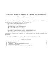
DEFINITION 5.4.1
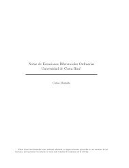
Let T1 : U → V and T2 : V → W be two linear transformations. 3 We define the
composition,orproduct, T2T1 : U → W by
(T2T1)(u) = T2(T1(u)) for all u ∈ U.
The composition is illustrated in Figure 5.4.1.
U
u
T 1
T 2T 1
V
T 1(u)
T 2
W
(T 2T 1)(u) T 2(T 1(u))
Figure 5.4.1: The composition of two linear transformations.
Our first result establishes that T2T1 is a linear transformation.
Theorem 5.4.2 Let T1 : U → V and T2 : V → W be linear transformations. Then T2T1 : U → W is a
linear transformation.
3
We assume that U,V, and W are either all real vector spaces or all complex vector spaces.