Systems of Linear Equations

1 Systems of linear equations
Linear systems
Systems of Linear Equations
Beifang Chen
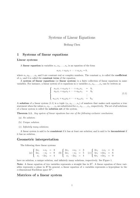
A linear equation in variables x1, x2, . . . , xn is an equation of the form
a1x1 + a2x2 + · · · + anxn = b,
where a1, a2, . . . , an and b are constant real or complex numbers. The constant ai is called the coefficient
of xi; and b is called the constant term of the equation.
A system of linear equations (or linear system) is a finite collection of linear equations in same
variables. For instance, a linear system of m equations in n variables x1, x2, . . . , xn can be written as
⎧
a11x1 + a12x2 + · · · + a1nxn = b1
⎪⎨ a21x1 + a22x2 + · · · + a2nxn = b2
(1.1)
⎪⎩
.
am1x1 + am2x2 + · · · + amnxn = bm
A solution of a linear system (1.1) is a tuple (s1, s2, . . . , sn) of numbers that makes each equation a true
statement when the values s1, s2, . . . , sn are substituted for x1, x2, . . . , xn, respectively. The set of all solutions
of a linear system is called the solution set of the system.
Theorem 1.1. Any system of linear equations has one of the following exclusive conclusions.
(a) No solution.
(b) Unique solution.
(c) Infinitely many solutions.
A linear system is said to be consistent if it has at least one solution; and is said to be inconsistent if
it has no solution.
Geometric interpretation
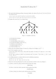
The following three linear systems
⎧
⎨ 2x1 +x2 = 3
(a) 2x1
⎩
x1
−x2
−2x2
=
=
0
4
⎧
⎨
(b)
⎩
2x1 +x2 = 3
2x1 −x2 = 5
x1 −2x2 = 4
⎧
⎨
(c)
⎩
2x1 +x2 = 3
4x1 +2x2 = 6
6x1 +3x2 = 9
have no solution, a unique solution, and infinitely many solutions, respectively. See Figure 1.
Note: A linear equation of two variables represents a straight line in R 2 . A linear equation of three variables
represents a plane in R 3 .In general, a linear equation of n variables represents a hyperplane in the
n-dimensional Euclidean space R n .
Matrices of a linear system
1

o
x 2
x 1
o
x 2
Figure 1: No solution, unique solution, and infinitely many solutions.
Definition 1.2. The augmented matrix of the general linear system (1.1) is the table
⎡
⎢
⎣
a11
a21
.
a12
a22
.
. . .
. . .
. ..
a1n
a2n
.
b1
b2
.
⎤
⎥
⎦
and the coefficient matrix of (1.1) is
am1 am2 . . . amn bm
⎡
⎢
⎣
a11 a12 . . . a1n
a21 a22 . . . a2n
.
. . .. .
am1 am2 . . . amn
2
⎤
⎥
⎦
x 1
o
x 2
x 1
(1.2)
(1.3)

Systems of linear equations can be represented by matrices. Operations on equations (for eliminating
variables) can be represented by appropriate row operations on the corresponding matrices. For example,
⎧
⎡
⎤
⎨ x1 +x2 −2x3 = 1
1 1 −2 1
2x1 −3x2 +x3 = −8
⎣ 2 −3 1 −8 ⎦
⎩
3x1 +x2 +4x3 = 7
3 1 4 7
⎧
⎨
⎩
⎧
⎨
⎩
⎧
⎨
⎩
[Eq 2] − 2[Eq 1]
[Eq 3] − 3[Eq 1]
x1 +x2 −2x3 = 1
−5x2 +5x3 = −10
−2x2 +10x3 = 4
⎧
⎨
⎩
(−1/5)[Eq 2]
(−1/2)[Eq 3]
x1 +x2 −2x3 = 1
x2 −x3 = 2
x2 −5x3 = −2
⎡
⎣
R2 − 2R1
R3 − 3R1
1 1 −2 1
0 −5 5 −10
0 −2 10 4
⎡
⎣
(−1/5)R2
(−1/2)R3
1 1 −2 1
0 1 −1 2
0 1 −5 −2
x1
[Eq 3] − [Eq 2]
+x2 −2x3 =
x2 −x3 =
1
2
⎡
1
⎣ 0
R3 − R2
1 −2
1 −1
1
2
−4x3 = −4
0 0 −4 −4
⎧
⎨
⎩
x1
(−1/4)[Eq 3]
+x2 −2x3
x2 −x3
=
=
1
2
(−1/4)R3
⎡
1 1 −2 1
⎣ 0 1 −1 2
x3 = 1
0 0 1 1
⎧
⎨
⎩
[Eq 1] + 2[Eq 3]
[Eq 2] + [Eq 3]
x1 +x2 = 3
x2 = 3
x3 = 1
⎡
⎣
R1 + 2R3
R2 + R3
1 1 0 3
0 1 0 3
0 0 1 1
[Eq 1] − [Eq 2] R1 − R2
⎡
1 0 0 0
⎣ 0 1 0 3
0 0 1 1
x1 = 0
x2 = 3
x3 = 1
Elementary row operations
Definition 1.3. There are three kinds of elementary row operations on matrices:
(a) Adding a multiple of one row to another row;
(b) Multiplying all entries of one row by a nonzero constant;
(c) Interchanging two rows.
Definition 1.4. Two linear systems in same variables are said to be equivalent if their solution sets are
the same. A matrix A is said to be row equivalent to a matrix B , written
A ∼ B,
if there is a sequence of elementary row operations that changes A to B.
3
⎤
⎦
⎤
⎦
⎤
⎦
⎤
⎦
⎤
⎦
⎤
⎦

Theorem 1.5. If the augmented matrices of two linear systems are row equivalent, then the two systems
have the same solution set. In other words, elementary row operations do not change solution set.
Proof. It is trivial for the row operations (b) and (c) in Definition 1.3. Consider the row operation (a) in
Definition 1.3. Without loss of generality, we may assume that a multiple of the first row is added to the
second row. Let us only exhibit the first two rows as follows
⎡
⎤
a11 a12 . . . a1n b1
⎢ a21 a22 ⎢
. . . a2n b2 ⎥
⎢
⎣
.
. . ..
⎥
(1.4)
. . ⎦
am1 am2 . . . amn bm
Do the row operation (Row 2) + c(Row 1). We obtain
⎡
a11
⎢ a21 ⎢ + ca11
⎢ a31 ⎢
⎣ .
a12
a22 + ca22
a32
.
. . .
. . .
. . .
. ..
a1n
a2n + ca2n
a3n
.
b1
b2 + cb1
b3
.
⎤
⎥
⎦
Let (s1, s2, . . . , sn) be a solution of (1.4), that is,
In particular,
Multiplying c to both sides of (1.7), we have
Adding both sides of (1.8) and (1.9), we obtain
am1 am2 . . . amn bm
(1.5)
ai1s1 + ai2s2 + · · · + ainsn = bi, 1 ≤ i ≤ m. (1.6)
a11s1 + a12x2 + · · · + a1nsn = b1, (1.7)
a21s1 + a21x2 + · · · + a2nsn = b2. (1.8)
ca11s1 + ca12 + · · · + ca1nsn = cb1. (1.9)
(a21 + ca11)s1 + (a22 + ca12)s2 + · · · + (a2n + ca1n)sn = b2 + cb1. (1.10)
This means that (s1, s2, . . . , sn) is a solution of (1.5).
Conversely, let (s1, s2, . . . , sn) be a solution of (1.5), i.e., (1.10) is satisfied and the equations of (1.6) are
satisfied except for i = 2. Since
a11s1 + a12x2 + · · · + a1nsn = b1,
multiplying c to both sides we have
Note that (1.10) can be written as
c(a11s1 + a12 + · · · + a1nsn) = cb1. (1.11)
(a21s1 + a22s2 + · · · + a2nsn) + c(a11s1 + a12s2 + · · · + a1nsn) = b2 + cb1. (1.12)
Subtracting (1.11) from (1.12), we have
This means that (s1, s2, . . . , sn) is a solution of (1.4).
a21s1 + a22s2 + · · · + a2nsn = b2.
4

2 Row echelon forms
Definition 2.1. A matrix is said to be in row echelon form if it satisfies the following two conditions:
(a) All zero rows are gathered near the bottom.
(b) The first nonzero entry of a row, called the leading entry of that row, is ahead of the first nonzero
entry of the next row.
A matrix in row echelon form is said to be in reduced row echelon form if it satisfies two more conditions:
(c) The leading entry of every nonzero row is 1.
(d) Each leading entry 1 is the only nonzero entry in its column.
A matrix in (reduced) row echelon form is called a (reduced) row echelon matrix.
Note 1. Sometimes we call row echelon forms just as echelon forms and row echelon matrices as echelon
matrices without mentioning the word “row.”
Row echelon form pattern
The following are two typical row echelon matrices.
⎡
⎢
⎣
• ∗ ∗ ∗ ∗ ∗ ∗ ∗ ∗
0 • ∗ ∗ ∗ ∗ ∗ ∗ ∗
0 0 0 0 • ∗ ∗ ∗ ∗
0 0 0 0 0 0 • ∗ ∗
0 0 0 0 0 0 0 0 0
0 0 0 0 0 0 0 0 0
⎤
⎥ ,
⎥
⎦
⎡
⎢
⎣
0 • ∗ ∗ ∗ ∗ ∗ ∗ ∗
0 0 0 0 • ∗ ∗ ∗ ∗
0 0 0 0 0 0 • ∗ ∗
0 0 0 0 0 0 0 0 •
0 0 0 0 0 0 0 0 0
0 0 0 0 0 0 0 0 0
where the circled stars • represent arbitrary nonzero numbers, and the stars ∗ represent arbitrary numbers,
including zero. The following are two typical reduced row echelon matrices.
⎡
1
⎢ 0
⎢ 0
⎢ 0
⎣ 0
0
1
0
0
0
∗
∗
0
0
0
∗
∗
0
0
0
0
0
1
0
0
∗
∗
∗
0
0
0
0
0
1
0
∗
∗
∗
∗
0
∗
∗
∗
∗
0
⎤
⎥ ,
⎥
⎦
⎡
0
⎢ 0
⎢ 0
⎢ 0
⎣ 0
1
0
0
0
0
∗
0
0
0
0
∗
0
0
0
0
0
1
0
0
0
∗
∗
0
0
0
0
0
1
0
0
0
0
0
0
0
⎤
0
0 ⎥
0 ⎥
1 ⎥
0 ⎦
0 0 0 0 0 0 0 0 0 0 0 0 0 0 0 0 0 0
Definition 2.2. If a matrix A is row equivalent to a row echelon matrix B, we say that A has the row
echelon form B; if B is further a reduced row echelon matrix, then we say that A has the reduced row
echelon form B.
Row reduction algorithm
Definition 2.3. A pivot position of a matrix A is a location of entries of A that corresponds to a leading
entry in a row echelon form of A. A pivot column (pivot row) is a column (row) of A that contains a
pivot position.
Algorithm 2.1 (Row Reduction Algorithm). (1) Begin with the leftmost nonzero column, which is
a pivot column; the top entry is a pivot position.
(2) If the entry of the pivot position is zero, select a nonzero entry in the pivot column, interchange the
pivot row and the row containing this nonzero entry.
(3) If the pivot position is nonzero, use elementary row operations to reduce all entries below the pivot
position to zero, (and the pivot position to 1 and entries above the pivot position to zero for reduced
row echelon form).
(4) Cover the pivot row and the rows above it; repeat (1)-(3) to the remaining submatrix.
5
⎤
⎥
⎦

Theorem 2.4. Every matrix is row equivalent to one and only one reduced row echelon matrix. In other
words, every matrix has a unique reduced row echelon form.
Proof. The Row Reduction Algorithm show the existence of reduced row echelon matrix for any matrix M.
We only need to show the uniqueness. Suppose A and B are two reduced row echelon forms for a matrix
M. Then the systems Ax = 0 and Bx = 0 have the same solution set. Write A = [aij] and B = [bij].
We first show that A and B have the same pivot columns. Let i1, . . . , ik be the pivot columns of A, and
let j1, . . . , jl be the pivot columns of B. Suppose i1 = j1, . . . , ir−1 = jr−1, but ir = jr. Assume ir < jr.
Then the irth row of A is
0, . . . , 0, 1, ar,ir+1, . . . , ar,jr, ar,jr+1, . . . , ar,n .
While the jrth row of B is
0, . . . , 0, 1, br,jr+1, . . . , br,n .
Since ir−1 = jr−1 and ir < jr, we have jr−1 < ir < jr. So xir is a free variable for Bx = 0. Let
ui1 = −b1,ir , . . . , uir−1 = −br−1,ir , uir = 1, and ui = 0 for i > ir.
Then u is a solution of Bx = 0, but is not a solution of Ax = 0. This is a contradiction. Of course, k = l.
Next we show that for 1 ≤ r ≤ k = l, we have
arj = brj, jr + 1 ≤ j ≤ jr+1 − 1.
Otherwise, we have ar0j0 = br0j0 such that r0 is smallest and then j0 is smallest. Set
uj0 = 1, ui1 = −a1,j0 , . . . , ur0 = −ar0j0 , and uj = 0 otherwise.
Then u is a solution of Ax = 0, but is not a solution of Bx = 0. This is a contradiction.
Solving linear system
Example 2.1. Find all solutions for the linear system
⎧
⎨
⎩
x1 +2x2 −x3 = 1
2x1 +x2 +4x3 = 2
3x1 +3x2 +4x3 = 1
Solution. Perform the row operations:
⎡
1
⎣ 2
2
1
−1
4
⎤
1
2 ⎦
R2 − 2R1
∼
⎡
⎣
3 3 4 1 R3 − 3R1
⎡
1
⎣ 0
2
1
−1
−2
⎤
1
0 ⎦
0 0 1 −2
R1 + R3
∼
⎡
⎣
R2 + 2R3
⎡
1
⎣ 0
0
1
0
0
⎤
7
−4 ⎦
0 0 1 −2
The system is equivalent to ⎧ ⎨
which means the system has a unique solution.
⎩
x1 = 7
x2 = −4
x3 = −2
6
1 2 −1 1
0 −3 6 0
0 −3 7 −2
1 2 0 −1
0 1 0 −4
0 0 1 −2
⎤
⎦
⎤
(−1/3)R2
∼
R3 − R2
⎦ R1 − 2R2
∼

Example 2.2. Solve the linear system
⎧
⎪⎨
Solution. Do the row operations:
⎡
⎢
⎣
1
1
4
−1
−1
−4
1
1
4
−1
1
0
⎤
2
0 ⎥
4 ⎦
−2 2 −2 1 −3
⎡
⎢
⎣
⎪⎩
1 −1 1 −1 2
0 0 0 1 −1
0 0 0 0 0
0 0 0 0 0
x1 −x2 +x3 −x4 = 2
x1 −x2 +x3 +x4 = 0
4x1 −4x2 +4x3 = 4
−2x1 +2x2 −2x3 +x4 = −3
R2 − R1
R3 − 4R1
∼
R4 + 2R1
⎤
⎡
⎢
⎣
⎥
⎦ R1 + R2
∼
The linear system is equivalent to x1 = 1 + x2 − x3
x4 = −1
1 −1 1 −1 2
0 0 0 2 −2
0 0 0 4 −4
0 0 0 −1 1
⎡
⎢
⎣
⎤
⎥
⎦
(1) [−1] [1] 0 1
0 0 0 (1) −1
0 0 0 0 0
0 0 0 0 0
(1/2)R2
R3 − 2R2
∼
R4 + (1/2)R2
We see that the variables x2, x3 can take arbitrary numbers; they are called free variables. Let x2 = c1,
x3 = c2, where c1, c2 ∈ R. Then x1 = 1 + c1 − c2, x4 = −1. All solutions of the system are given by
⎧
x1 ⎪⎨
= 1 + c1 − c2
The general solutions may be written as
⎡
x1
⎢ x2
x = ⎢
⎣ x3
⎤
⎥
⎦ =
⎡
⎢
⎣
1
0
0
−1
x4
⎪⎩
⎤
x2 = c1
x3 = c2
x4 = −1
⎡
⎥ ⎢
⎥
⎦ + c1 ⎢
⎣
1
1
0
0
⎤
⎡
⎥ ⎢
⎥
⎦ + c2 ⎢
⎣
Set c1 = c2 = 0, i.e., set x2 = x3 = 0, we have a particular solution
x =
⎡
⎢
⎣
1
0
0
−1
For the corresponding homogeneous linear system Ax = 0, i.e.,
we have ⎡
⎢
⎣
⎧
⎪⎨
⎪⎩
⎤
⎥
⎦ .
−1
0
1
0
x1 −x2 +x3 −x4 = 0
x1 −x2 +x3 +x4 = 0
4x1 −4x2 +4x3 = 0
−2x1 +2x2 −2x3 +x4 = 0
1 −1 1 −1 0
1 −1 1 1 0
4 −4 4 0 0
−2 2 −2 1 0
⎤
⎥
⎦ ∼
7
⎡
⎢
⎣
⎤
⎤
⎥
⎦
⎥
⎦ , where c1, c2 ∈ R.
(1) [−1] [1] −1 0
0 0 0 (1) 0
0 0 0 0 0
0 0 0 0 0
⎤
⎥
⎦

Set c1 = 1, c2 = 0, i.e., x2 = 1, x3 = 0, we obtain one basic solution
for the homogeneous system Ax = 0.
x =
Set c1 = 0, c2 = 1, i.e., x2 = 0, x3 = 1, we obtain another basic solution
for the homogeneous system Ax = 0.
x =
⎡
⎢
⎣
⎡
⎢
⎣
1
1
0
0
−1
0
1
0
Example 2.3. The linear system with the augmented matrix
⎡
1
⎣ 2
2
1
−1
5
⎤
1
2 ⎦
3 3 4 1
has no solution because its augmented matrix has the row echelon form
⎡
(1) 2 −1 1
⎤
⎣ 0 (−3) [7] 0 ⎦
0 0 0 −2
The last row represents a contradictory equation 0 = −2.
Theorem 2.5. A linear system is consistent if and only if the row echelon form of its augmented matrix
contains no row of the form 0, . . . , 0 b , where b = 0.
Example 2.4. Solve the linear system whose augmented matrix is
⎡
0
⎢
A = ⎢ 3
⎣ 1
0
6
2
1
0
0
−1
3
1
2
−3
−1
1
2
0
⎤
0
7 ⎥
1 ⎦
2 4 −2 4 −6 −5 −4
Solution. Interchanging Row 1 and Row 2, we have
⎡
1
⎢ 3
⎣ 0
2
6
0
0
0
1
1
3
−1
−1
−3
2
0
2
1
⎤
1
7 ⎥
0 ⎦
2 4 −2 4 −6 −5 −4
⎡
⎢
⎣
⎡
⎢
⎣
⎤
⎥
⎦
⎤
⎥
⎦
1 2 0 1 −1 0 1
0 0 0 0 0 2 4
0 0 1 −1 2 1 0
0 0 −2 2 −4 −5 −6
1 2 0 1 −1 0 1
0 0 1 −1 2 1 0
0 0 0 0 0 2 4
0 0 −2 2 −4 −5 −6
8
⎤
R2 − 3R1
∼
R4 − 2R1
⎥
⎦ R2 ↔ R3
∼
⎤
⎥
⎦ R4 + 2R2
∼

⎡
⎢
⎣
⎡
⎢
⎣
Then the system is equivalent to ⎧ ⎨
1 2 0 1 −1 0 1
0 0 1 −1 2 1 0
0 0 0 0 0 2 4
0 0 0 0 0 −3 −6
1 2 0 1 −1 0 1
0 0 1 −1 2 1 0
0 0 0 0 0 1 2
⎤
⎥
⎦
⎤
R4 + 3
2 R3
∼
1
2 R3
⎥
⎦ R2 − R3
∼
0 0
⎡
(1)
⎢ 0
⎣ 0
0
[2]
0
0
0
0
(1)
0
0
1
[−1]
0
0
−1
[2]
0
0
0
0
(1)
1
−2
2
⎤
⎥
⎦
0 0 0 0 0 0 0
⎩
x1 = 1 − 2x2 − x4 + x5
x3 = −2 + x4 − 2x5
x6 = 2
The unknowns x2, x4 and x5 are free variables.
Set x2 = c1, x4 = c2, x5 = c3, where c1, c2, c3 are arbitrary. The general solutions of the system are given
by ⎧⎪
x1 = 1 − 2c1 − c2 + c3
x2 = c1
⎨
x3 = −2 + c2 − 2c3
The general solution may be written as
⎡ ⎤ ⎡ ⎤ ⎡
x1 1
⎢ x2 ⎥ ⎢
⎢ ⎥ ⎢ 0 ⎥ ⎢
⎥ ⎢
⎢ x3 ⎥ ⎢
⎢ ⎥
⎢ x4 ⎥ = ⎢ −2 ⎥ ⎢
⎥
⎢
⎢ ⎥ ⎢ 0 ⎥ + c1 ⎢
⎥ ⎢
⎣ x5 ⎦ ⎣ 0 ⎦ ⎣
2
x6
⎪⎩
x4 = c2
x5 = c3
x6 = 2
−2
1
0
0
0
0
⎤
⎡
⎥ ⎢
⎥ ⎢
⎥ ⎢
⎥ + c2 ⎢
⎥ ⎢
⎦ ⎣
−1
0
1
1
0
0
⎤
⎡
⎥ ⎢
⎥ ⎢
⎥ ⎢
⎥ + c3 ⎢
⎥ ⎢
⎦ ⎣
1
0
−2
0
1
0
⎤
⎥ , c1, c2, c3 ∈ R.
⎥
⎦
Definition 2.6. A variable in a consistent linear system is called free if its corresponding column in the
coefficient matrix is not a pivot column.
Theorem 2.7. For any homogeneous system Ax = 0,
3 Vector Space R n
#{variables} = #{pivot positions of A} + #{free variables}.
Vectors in R 2 and R 3
Let R 2 be the set of all ordered pairs (u1, u2) of real numbers, called the 2-dimensional Euclidean
space. Each ordered pair (u1, u2) is called a point in R 2 . For each point (u1, u2) we associate a column
u1
u2
called the vector associated to the point (u1, u2). The set of all such vectors is still denoted by R 2 . So by
a point in the Euclidean space R 2 we mean an ordered pair
(x, y)
9
,

and, by a vector in the vector space R 2 we mean a column
Similarly, we denote by R 3 the set of all tuples
x
y
.
(u1, u2, u3)
of real numbers, called points in the Euclidean space R3 . We still denote by R3 the set of all columns
⎡ ⎤
called vectors in R3 . For example, (2, 3, 1), (−3, 1, 2), (0, 0, 0) are points in R3 , while
⎡
2
⎤ ⎡ ⎤
−3
⎡
0
⎤
⎣ 3 ⎦ , ⎣ 1 ⎦ , ⎣ 0 ⎦
1 2 0
are vectors in the vector space R 3 .
⎣
Definition 3.1. The addition, subtraction, and scalar multiplication for vectors in R2 are defined by
u1
v1
+
u1 + v1
=
,
u2
u1
u2
u3
v2
v1
−
v2
u1
c
u2
v3
u1
u2
u3
⎦ ,
u2 + v2
u1 − v1
=
cu1
=
cu2
u2 − v2
Similarly, the addition, subtraction, and scalar multiplication for vectors in R3 are defined by
⎡
⎣ u1
u2
⎤ ⎡
⎦ + ⎣ v1
v2
⎤ ⎡
⎦ = ⎣ u1 + v1
u2 + v2
⎤
⎦ ,
Vectors in R n
⎡
⎣
u1
u2
u3
⎤
⎡
⎦ − ⎣
c
⎡
⎣ u1
u2
u3
v1
v2
v3
⎤
⎤
⎦ =
⎡
⎦ = ⎣
⎡
⎣ cu1
cu2
cu3
.
u3 + v3
u1 − v1
u2 − v2
u3 − v3
Definition 3.2. Let Rn be the set of all tuples (u1, u2, . . . , un) of real numbers, called points in the ndimensional
Euclidean space Rn . We still use Rn to denote the set of all columns
⎡ ⎤
⎢
⎣
u1
u2
.
un
10
⎥
⎦
⎤
⎦ .
,
⎤
⎦ ,

of real numbers, called vectors in the n-dimensional vector space Rn . The vector
⎡ ⎤
0
⎢ 0 ⎥
0 = ⎢ ⎥
⎣ . ⎦
0
is called the zero vector in Rn . The addition and the scalar multiplication in Rn are defined by
⎡ ⎤ ⎡ ⎤ ⎡ ⎤
⎢
⎣
u1
u2
.
un
⎥
⎦ +
⎢
⎣
⎡
⎢
c ⎢
⎣
u1
u2
.
un
v1
v2
.
vn
⎥
⎦ =
⎢
⎣
cun
u1 + v1
u1 + v2
.
un + vn
⎤
⎥
⎦ =
⎡ ⎤
cu1
⎢ cu2 ⎥
⎢ ⎥
⎢ ⎥
⎣ . ⎦ .
Proposition 3.3. For vectors u, v, w in R n and scalars c, d in R,
(1) u + v = v + u,
(2) (u + v) + w = u + (v + w),
(3) u + 0 = u,
(4) u + (−u) = 0,
(5) c(u + v) = cu + cv,
(6) (c + d)u = cu + du
(7) c(du) = (cd)u
(8) 1u = u.
Subtraction can be defined in R n by
Linear combinations
u − v = u + (−v).
Definition 3.4. A vector v in R n is called a linear combination of vectors v1, v2, . . . , vk in R n if there
exist scalars c1, c2, . . . , ck such that
v = c1v1 + c2v2 + · · · + ckvk.
The set of all linear combinations of v1, v2, . . . , vk is called the span of v1, v2, . . . , vk, denoted
Span {v1, v2, . . . , vk}.
Example 3.1. The span of a single nonzero vector in R3 is a straight line through the origin. For instance,
⎧⎡
⎨
Span ⎣
⎩
3
⎤⎫
⎬
−1 ⎦
⎭
2
=
⎧
⎨
⎩ t
⎡
⎣ 3
⎤ ⎫
⎬
−1 ⎦ : t ∈ R
⎭
2
11
⎥
⎦ ,

is a straight line through the origin, having the parametric form
⎧
⎨
⎩
x1 = 3t
x2 = −t
x3 = 2t
, t ∈ R.
Eliminating the parameter t, the parametric equations reduce to two equations about x1, x2, x3,
x1 +3x2 = 0
2x2 +x3 = 0
Example 3.2. The span of two linearly independent vectors in R3 is a plane through the origin. For
instance,
⎧⎡
⎨
Span ⎣
⎩
3
⎤ ⎡
−1 ⎦ , ⎣
2
1
2
−1
⎤⎫
⎬
⎦
⎭ =
⎧
⎨
⎩ s
⎡
⎣ 1
2
−1
⎤ ⎡
⎦ + t ⎣ 3
⎤ ⎫
⎬
−1 ⎦ : s, t ∈ R
⎭
2
is a plane through the origin, having the following parametric form
⎧
⎨
⎩
x1 = s +3t
x2 = 2s −t
x3 = −s +2t
Eliminating the parameters s and t, the plane can be described by a single equation
Example 3.3. Given vectors in R3 ,
⎡ ⎤ ⎡
1
v1 = ⎣ 2 ⎦ , v2 = ⎣
0
3x1 − 5x2 − 7x3 = 0.
1
1
1
⎤
⎡
⎦ , v3 = ⎣
1
0
1
⎤
⎡
⎦ , v4 = ⎣
(a) Every vector b = [b1, b2, b3] T in R 3 is a linear combination of v1, v2, v3.
(b) The vector v4 can be expressed as a linear combination of v1, v2, v3, and it can be expressed in one
and only one way as a linear combination
v = 2v1 − v2 + 3v3.
(c) The span of {v1, v2, v3} is the whole vector space R 3 .
Solution. (a) Let b = x1v1 + x2v2 + x3v3. Then the vector equation has the following matrix form
⎡
1
⎣ 2
1
1
⎤ ⎡
1 x1
0 ⎦ ⎣ x2
⎤ ⎡
b1
⎦ = ⎣ b2
⎤
⎦
0 1 1
Perform row operations:
⎡
1
⎣ 2
1
1
1
0
b1
b2
⎤ ⎡
1
⎦ ∼ ⎣ 0
1
−1
1
−2
b1
b2 − 2b1
⎤
⎦ ∼
0 1 1 b3 0 1 1 b3
⎡
⎣ 1 0 −1 b2
0 1 2
− b1
2b1 − b2
⎤ ⎡
⎦ ∼ ⎣
0 0 −1 b3 + b2 − 2b1
1 0 0 b1
0 1 0
− b3
−2b1 + b2 + 2b3
0 0 1 2b1 − b2 − b3
Thus
x1 = b1 − b3, x2 = −2b1 + b2 + 2b3, x3 = 2b1 − b2 − b3.
So b is a linear combination of v1, v2, v3.
(b) In particular, v4 = 2v1 − v2 + 3v3.
(c) Since b is arbitrary, we have Span {v1, v2, v3} = R 3 .
12
x3
b3
4
3
2
⎤
⎦ .
⎤
⎦

Example 3.4. Consider vectors in R3 ,
⎡ ⎤ ⎡
1
v1 = ⎣ −1 ⎦ , v2 = ⎣
1
−1
2
1
⎤
⎡
⎦ , v3 = ⎣
1
1
5
⎤
⎡
⎦ ; u = ⎣
1
2
7
⎤
⎡
⎦ , v = ⎣
(a) The vector u can be expressed as linear combinations of v1, v2, v3 in more than one ways. For instance,
u = v1 + v2 + v3 = 4v1 + 3v2 = −2v1 − v2 + 2v3.
(b) The vector v can not be written as a linear combination of v1, v2, v3.
Geometric interpretation of vectors
Multiplication of matrices
Definition 3.5. Let A be an m × n matrix and B an n × p matrix,
⎡
⎢
A = ⎢
⎣
a11
a21
.
a12
a22
.
. . .
. . .
a1n
a2n
.
⎤
⎥ ,
⎦
⎡
⎢
B = ⎢
⎣
b11
b21
.
b12
b22
.
. . .
. . .
b1p
b2p
.
⎤
⎥
⎦ .
am1 am2 . . . amn
The product (or multiplication) of A and B is an m × p matrix
⎡
⎢
C = ⎢
⎣
c11
c21
.
c12
c22
.
. . .
. . .
c1p
c2p
.
⎤
⎥
⎦
cm1 cm2 . . . cmp
whose (i, k)-entry cik, where 1 ≤ i ≤ m and 1 ≤ k ≤ p, is given by
cik =
bn1 an2 . . . bnp
n
aijbjk = ai1b1k + ai2b2k + · · · + ainbnk.
j=1
Proposition 3.6. Let A be an m × n matrix, whose column vectors are denoted by a1, a2, . . . , an. Then for
any vector v in Rn ,
⎡ ⎤
Proof. Write
Then
⎢
Av = [a1, a2, . . . , an] ⎢
⎣
⎡
⎢
A = ⎢
⎣
⎡
⎢
a1 = ⎢
⎣
a11
a21
.
am1
v1
v2
.
vn
a11 a12 . . . a1n
a21 a22 . . . a2n
.
.
am1 am2 . . . amn
⎤
⎡
⎥
⎦ , a2
⎢
= ⎢
⎣
⎥
⎦ = v1a1 + v2a2 + · · · + vnan.
a12
a22
.
am2
13
.
⎤
⎤
⎡
⎥ ⎢
⎥ ⎢
⎥ , v = ⎢
⎦ ⎣
v1
v2
.
vn
⎡
⎥
⎦ , . . . , an
⎢
= ⎢
⎣
⎤
⎥
⎦ .
a1n
a2n
.
amn
⎤
⎥
⎦ .
1
1
1
⎤
⎦

Thus
Av =
=
=
⎡
⎢
⎣
⎡
⎢
⎣
⎡
⎢
⎣
⎢
= v1 ⎢
⎣
a11 a12 . . . a1n
a21 a22 . . . a2n
.
.
am1 am2 . . . amn
.
⎤ ⎡
⎥ ⎢
⎥ ⎢
⎥ ⎢
⎦ ⎣
a11v1 + a12v2 + · · · + a1nvn
a21v1 + a22v2 + · · · + a2nvn
.
v1
v2
.
vn
am1v1 + am2v2 + · · · + amnvn
a11v1
a21v1
.
am1v1
⎡
a11
a21
.
.
am1
⎤
⎡
⎥
⎦ +
⎢
⎣
⎤
⎥ ⎢
⎥ ⎢
⎥ + v2 ⎢
⎦ ⎣
a12v2
a22v2
.
am2v2
⎡
a12
a22
.
am2
⎤
= v1a1 + v2a2 + · · · + vnan.
⎤
⎥
⎦
⎤
⎥
⎦
⎡
⎥ ⎢
⎥ ⎢
⎥ + · · · + ⎢
⎦ ⎣
⎤
⎥ ⎢
⎥ ⎢
⎥ + · · · + vn ⎢
⎦ ⎣
a1nvn
a2nvn
.
amnvn
Theorem 3.7. Let A be an m × n matrix. Then for any vectors u, v in R n and scalar c,
(a) A(u + v) = Au + Av,
(b) A(cu) = cAu.
4 The four expressions of a linear system
A general system of linear equations can be written as
⎧
⎪⎨
a11x1 + a12x2 + · · · + a1nxn
a21x1 + a22x2 + · · · + a2nxn
=
=
b1
b1
⎪⎩
We introduce the column vectors:
⎡ ⎤
a1 =
⎢
⎣
a11
.
am1
and the coefficient matrix:
am1x1 + am2x2 + · · · + amnxn = bm
⎡
⎥
⎢
⎦ , . . . , an = ⎣
⎡
⎢
A = ⎢
⎣
a1n
.
amn
⎤
a11 a12 . . . a1n
a21 a22 . . . a2n
.
.
am1 am2 . . . amn
Then the linear system (4.1) can be expressed by
⎡
⎥ ⎢
⎦ ; x = ⎣
.
14
⎤
.
x1
.
xn
⎤
⎡
a1n
a2n
.
amn
⎤
⎥
⎦
⎤
⎥
⎦
⎡
⎥ ⎢
⎦ ; b = ⎣
⎥
⎦ = [ a1, a2, . . . , an ].
b1
.
bm
⎤
⎥
⎦ ;
(4.1)

(a) The vector equation form:
(b) The matrix equation form:
x1a1 + x2a2 + · · · + xnan = b,
Ax = b,
(c) The augmented matrix form: a1, a2, . . . , an | b .
Theorem 4.1. The system Ax = b has a solution if and only if b is a linear combination of the column
vectors of A.
Theorem 4.2. Let A be an m × n matrix. The following statements are equivalent.
(a) For each b in R m , the system Ax = b has a solution.
(b) The column vectors of A span R m .
(c) The matrix A has a pivot position in every row.
Proof. (a) ⇔ (b) and (c) ⇒ (a) are obvious.
(a) ⇒ (c): Suppose A has no pivot position for at least one row; that is,
A ρ1 ρ2
∼ A1 ∼ · · · ρk−1 ρk
∼ Ak−1 ∼ Ak,
where ρ1, ρ2, . . . , ρk are elementary row operations, and Ak is a row echelon matrix. Let em = [0, . . . , 0, 1] T .
Clearly, the system [A | en] is inconsistent. Let ρ ′ i denote the inverse row operation of ρi, 1 ≤ i ≤ k. Then
[Ak | em] ρ′
k
∼ [Ak−1 | b1] ρ′
k−1
∼ · · ·
Thus, for b = bk, the system [A | b] has no solution, a contradiction.
ρ ′
2
∼ [A1 | bk−1] ρ′
1
∼ [A | bk].
Example 4.1. The following linear system has no solution for some vectors b in R3 .
⎧
⎨ 2x2 +2x3 +3x4 = b1
⎩
2x1 +4x2 +6x3 +7x4 = b2
x1 +x2 +2x3 +2x4 = b3
The row echelon matrix of the coefficient matrix for the system is given by
⎡
0
⎣ 2
1
2
4
1
2
6
2
3
7
2
⎤
⎦ R1 ↔ R3
∼
⎡
1
⎣ 2
0
1
4
2
2
6
2
⎤
2
7 ⎦
3
R2
⎡
1
⎣ 0
0
1
2
2
2
2
2
2
3
3
⎤
⎦ R3 − R2
∼
⎡
1
⎣ 0
0
1
2
0
2
2
0
− 2R1
∼
⎤
2
3 ⎦ .
0
Then the following systems have no solution.
⎡
1
⎣ 0
0
⎡
1
⎣ 2
0
1
2
0
1
4
2
2
2
0
2
6
2
2
3
0
2
7
3
⎤
0
0 ⎦
1
⎤
0
0 ⎦
1
R3 + R2
∼
R3 ↔ R1
∼
Thus the original system has no solution for b1 = 1, b2 = b3 = 0.
15
⎡
⎣
⎡
⎣
1 1 2 2 0
0 2 2 3 0
0 2 2 3 1
0 2 2 3 1
2 4 6 7 0
1 1 2 2 0
⎤
⎦ R2 + 2R1
∼
⎤
⎦ .

5 Solution structure of a linear System
Homogeneous system
A linear system is called homogeneous if it is in the form Ax = 0, where A is an m × n matrix and 0
is the zero vector in R m . Note that x = 0 is always a solution for a homogeneous system, called the zero
solution (or trivial solution); solutions other than the zero solution 0 are called nontrivial solutions.
Theorem 5.1. A homogeneous system Ax = 0 has a nontrivial solution if and only if the system has at
least one free variable. Moreover,
# pivot positions + # free variables = # variables .
Example 5.1. Find the solution set for the nonhomogeneous linear system
⎧
⎪⎨
⎪⎩
x1 −x2 +x4 +2x5 = 0
−2x1 +2x2 −x3 −4x4 −3x5 = 0
x1 −x2 +x3 +3x4 +x5 = 0
−x1 +x2 +x3 +x4 −3x5 = 0
Solution. Do row operations to reduce the coefficient matrix to the reduced row echelon form:
⎡
1
⎢ −2
⎣ 1
−1
2
−1
0
−1
1
1
−4
3
2
−3
1
⎤
⎥
⎦
R2 + 2R1
R3 − R1
∼
−1
⎡
1
⎢ 0
⎣ 0
1
−1
0
0
1
0
−1
1
1
1
−2
2
−3
⎤
2
1 ⎥
−1 ⎦
R4 + R1
(−1)R2
R3 + R2
∼
0
⎡
(1)
⎢ 0
⎣ 0
0
[−1]
0
0
1
0
(1)
0
2
1
[2]
0
−1 R4 + R2
⎤
2
[−1] ⎥
0 ⎦
0 0 0 0 0
Then the homogeneous system is equivalent to
x1 = x2 −x4 −2x5
x5
c3
x3 = −2x4 +x5
The variables x2, x4, x5 are free variables. Set x2 = c1, x4 = c2, x5 = c3. We have
⎡
x1
⎢ x2 ⎢ x3 ⎢
⎣ x4
⎤
⎥
⎦ =
⎡
c1 − c2 − 2c3
⎢ c1 ⎢ −2c2 ⎢ + c3
⎣ c2
⎤ ⎡ ⎤ ⎡ ⎤ ⎡
1 −1 −2
⎥ ⎢
⎥ ⎢ 1 ⎥ ⎢
⎥ ⎢ 0 ⎥ ⎢
⎥ ⎢ 0
⎥ = c1 ⎢ 0 ⎥ + c2 ⎢ −2 ⎥ + c3 ⎢ 1
⎦ ⎣ 0 ⎦ ⎣ 1 ⎦ ⎣ 0
0
0
1
Set x2 = 1, x4 = 0, x5 = 0, we obtain the basic solution
⎡
⎢
v1 = ⎢
⎣
16
1
1
0
0
0
⎤
⎥
⎦ .
⎤
⎥
⎦ .

Set x2 = 0, x4 = 1, x5 = 0, we obtain the basic solution
⎡
⎢
v2 = ⎢
⎣
Set x2 = 0, x4 = 0, x5 = 1, we obtain the basic solution
The general solution of the system is given by
⎡
⎢
v3 = ⎢
⎣
In other words, the solution set is Span {v1, v2, v3}.
−1
0
−2
1
0
−2
0
1
0
1
⎤
⎥
⎦ .
⎤
⎥
⎦ .
x = c1v1 + c2v2 + c3v3, c1, c2, c3, ∈ R.
Theorem 5.2. Let Ax = 0 be a homogeneous system. If u and v are solutions, then the addition and the
scalar multiplication
u + v, cu
are also solutions. Moreover, any linear combination of solutions for a homogeneous system is again a
solution.
Theorem 5.3. Let Ax = 0 be a homogeneous linear system, where A is an m × n matrix with p pivot
positions. Then system has n −p free variables and n −p basic solutions. The basic solutions can be obtained
as follows: Setting one free variable equal to 1 and all other free variables equal to 0.
Nonhomogeneous systems
A linear system Ax = b is called nonhomogeneous if b = 0. The homogeneous linear system Ax = 0
is called its corresponding homogeneous linear system.
Proposition 5.4. Let u and v be solutions of a nonhomogeneous system Ax = b. Then the difference
u − v
is a solution of the corresponding homogeneous system Ax = 0.
Theorem 5.5 (Structure of Solution Set). Let xnonh be a solution of a nonhomogeneous system Ax = b.
Let xhom be the general solutions of the corresponding homogeneous system Ax = 0. Then
are the general solutions of Ax = b.
x = xnonh + xhom
Example 5.2. Find the solution set for the nonhomogeneous linear system
⎧
⎪⎨
⎪⎩
x1 −x2 +x4 +2x5 = −2
−2x1 +2x2 −x3 −4x4 −3x5 = 3
x1 −x2 +x3 +3x4 +x5 = −1
−x1 +x2 +x3 +x4 −3x5 = 3
17

Solution. Do row operations to reduce the augmented matrix to the reduced row echelon form:
⎡
1
⎢ −2
⎣ 1
−1
2
−1
0
−1
1
1
−4
3
2
−3
1
⎤
−2
3 ⎥
−1 ⎦
R2 + 2R1
R3 − R1
∼
⎡
⎢
⎣
1
0
0
−1
0
0
0
−1
1
1
−2
2
2
1
−1
−2
−1
1
⎤
⎥
⎦
(−1)R2
R3 + R2
∼
−1 1 1 1 −3 3 R4 + R1 0 0 1 2 −1 1 R4 + R2
⎡
(1)
⎢ 0
⎣ 0
[−1]
0
0
0
(1)
0
1
[2]
0
2
[−1]
0
−2
1
0
⎤
⎥
⎦
0 0 0 0 0 0
Then the nonhomogeneous system is equivalent to
x1 = −2 +x2 −x4 −2x5
x5
c3
x3 = 1 −2x4 +x5
The variables x2, x4, x5 are free variables. Set x2 = c1, x4 = c2, x5 = c3. We obtain the general solutions
⎡ ⎤
x1
⎢ x2 ⎥
⎢ ⎥
⎢ x3 ⎥
⎢ ⎥
⎣ x4 ⎦ =
⎡
⎤
−2 + c1 − c2 − 2c3
⎢ c1 ⎥
⎢
⎥
⎢ 1 − 2c2 + c3 ⎥
⎣ c2 ⎦ =
⎡ ⎤ ⎡ ⎤ ⎡ ⎤ ⎡ ⎤
−2 1 −1 −2
⎢ 0 ⎥ ⎢
⎥ ⎢ 1 ⎥ ⎢
⎥ ⎢ 0 ⎥ ⎢
⎥ ⎢ 0 ⎥
⎢ 1 ⎥ + c1 ⎢ 0 ⎥ + c2 ⎢ −2 ⎥ + c3 ⎢ 1 ⎥
⎣ 0 ⎦ ⎣ 0 ⎦ ⎣ 1 ⎦ ⎣ 0 ⎦
0 0
0
1
,
or
x = v + c1v1 + c2v2 + c3v3, c1, c2, c3 ∈ R,
called the parametric form of the solution set. In particular, setting x2 = x4 = x5 = 0, we obtain the
particular solution
The solution set of Ax = b is given by
⎡
⎢
v = ⎢
⎣
−2
0
1
0
0
⎤
⎥
⎦ .
S = v + Span {v1, v2, v3}.
Example 5.3. The augmented matrix of the nonhomogeneous system
⎧
⎪⎨
⎪⎩
has the reduced row echelon form ⎡
x1 −x2 +x3 +3x4 +3x5 +4x6 = 2
−2x1 +2x2 −x3 −3x4 −4x5 −5x6 = −1
−x1 +x2 −x5 −4x6 = −5
−x1 +x2 +x3 +3x4 +x5 −x6 = −2
⎢
⎣
(1) [−1] 0 0 1 0 −3
0 0 (1) [3] [2] 0 −3
0 0 0 0 0 (1) 2
0 0 0 0 0 0 0
Then a particular solution xp for the system and the basic solutions of the corresponding homogeneous
system are given by
⎡ ⎤
−3
⎢ 0 ⎥
⎢
xp = ⎢ −3 ⎥
⎢ 0 ⎥ ,
⎥
⎣ 0 ⎦
⎡ ⎤
1
⎢ 1 ⎥
⎢
v1 = ⎢ 0 ⎥
⎢ 0 ⎥ ,
⎥
⎣ 0 ⎦
⎡
0
⎢ 0
⎢
v2 = ⎢ −3
⎢ 1
⎣ 0
⎤
⎥ ,
⎥
⎦
⎡
−1
⎢ 0
⎢
v3 = ⎢ −2
⎢ 0
⎣ 1
⎤
⎥ .
⎥
⎦
2
0
0
0
18
⎤
⎥
⎦ .

The general solution of the system is given by
x = xp + c1v1 + c2v2 + c3v3.
Example 5.4. For what values of a and b the linear system
⎧
⎨
⎩
x1 +2x2 +ax3 = 0
2x1 +bx2 = 0
3x1 +2x2 +x3 = 0
has nontrivial solutions. Answer: 8a + (3a − 1)(b − 4) = 0.
6 Linear dependence and independence
Lecture 6
Definition 6.1. Vectors v1, v2, . . . , vk in R n are said to be linearly independent provided that, whenever
c1v1 + c2v2 + · · · + ckvk = 0
for some scalars c1, c2, . . . , ck, then c1 = c2 = · · · = ck = 0.
The vectors v1, v2, . . . , vk are called linearly dependent if there exist constants c1, c2, . . . , ck, not all
zero, such that
c1v1 + c2v2 + · · · + ckvk = 0.
⎡
Example 6.1. The vectors v1 = ⎣ 1
⎤ ⎡
1 ⎦ , v2 = ⎣
−1
−1
1
⎤ ⎡
⎦ , v3 = ⎣
2
1
3
⎤
⎦ in R
1
3 are linearly independent.
Solution. Consider the linear system
⎡
x1 ⎣
⎤ ⎡
1 −1
1 ⎦ + x2 ⎣ 1
⎤ ⎡
1
⎦ + x3 ⎣ 3
⎤ ⎡
0
⎦ = ⎣ 0
⎤
⎦
−1
2 1 0
⎡
⎣
1
1
−1
1
1
3
⎤ ⎡
1
⎦ ∼ ⎣ 0
−1
2
⎤ ⎡
1 1
2 ⎦ ∼ ⎣ 0
0
1
⎤
0
0 ⎦
−1 2 1 0 1 2 0 0 1
The system has the only zero solution x1 = x2 = x3 = 0. Thus v1, v2, v3 are linearly independent.
⎡
Example 6.2. The vector v1 = ⎣ 1
⎤ ⎡
−1 ⎦ , v2 = ⎣
1
−1
2
⎤ ⎡
⎦ , v3 = ⎣
2
−1
3
⎤
⎦ in R
5
3 are linearly dependent.
Solution. Consider the linear system
⎡
x1 ⎣ 1
⎤ ⎡
−1 ⎦ + x2 ⎣
1
−1
2
⎤ ⎡
⎦ + x3 ⎣
2
−1
⎤ ⎡
3 ⎦ = ⎣
5
0
⎤
0 ⎦
0
⎡
1
⎣ −1
−1
2
⎤ ⎡
−1 1
3 ⎦ ∼ ⎣ 0
−1
1
⎤ ⎡
−1 1
2 ⎦ ∼ ⎣ 0
−1
1
−1
2
⎤
⎦
1 2 5 0 3 6 0 0 0
The system has one free variable. There is nonzero solution. Thus v1, v2, v3 are linearly dependent.
⎡
Example 6.3. The vectors ⎣ 1
⎤ ⎡
1 ⎦ , ⎣
−1
1
⎤ ⎡
−1 ⎦ , ⎣
1
−1
1
⎤ ⎡
⎦ , ⎣
1
1
3
⎤
⎦ in R
−3
3 are linearly dependent.
19

Theorem 6.2. The basic solutions of any homogeneous linear system are linearly independent.
Proof. Let v1, v2, . . . , vk be basic solutions of a linear system Ax = 0, corresponding to free variables
, xj2 , . . . , xjk . Consider the linear combination
xj1
c1v1 + c2v2 + · · · + ckvk = 0.
Note that the ji coordinate of c1v1 + c2v2 + · · · + ckvk is cji, 1 ≤ i ≤ k. It follows that cji = 0 for all
1 ≤ i ≤ k. This means that v1, v2, . . . , vk are linearly independent.
Theorem 6.3. Any set of vectors containing the zero vector 0 is linearly dependent.
Theorem 6.4. Let v1, v2, . . . , vp be vectors in R n . If p > n, then v1, v2, . . . , vp are linearly dependent.
Proof. Let A = [v1, v2, . . . , vp]. Then A is an n × p matrix, and the equation Ax = 0 has n equations in p
unknowns. Recall that for the matrix A the number of pivot positions plus the number of free variables is
equal to p, and the number of pivot positions is at most n. Thus, if p > n, there must be some free variables.
Hence Ax = 0 has nontrivial solutions. This means that the column vectors of A are linearly dependent.
Theorem 6.5. Let S = {v1, v2, . . . , vp} be a set of vectors in R n , (p ≥ 2). Then S is linearly dependent if
and only if one of vectors in S is a linear combination of the other vectors.
Moreover, if S is linearly dependent and v1 = 0, then there is a vector vj with j ≥ 2 such that vj is a
linear combination of the preceding vectors v1, v2, . . . , vj−1.
Note 2. The condition v1 = 0 in the above theorem can not be deleted. For example, the set
0
v1 =
0
1
, v2 =
1
is linearly dependent. But v2 is not a linear combination of v1.
Theorem 6.6. The column vectors of a matrix A are linearly independent if and only if the linear system
has the only zero solution.
Ax = 0
Proof. Let A = [a1, a2, . . . , an]. Then the linear system Ax = 0 is the vector equation
x1a1 + x2a2 + · · · + xnan = 0.
Then a1, a2, . . . , an are linear independent is equivalent to that the system has only the zero solution.
20