- Page 2 and 3:
HANDBOOK OF CIVIL ENGINEERING CALCU
- Page 4 and 5:
HANDBOOK OF CIVIL ENGINEERING CALCU
- Page 6 and 7:
To civil engineers—everywhere: Th
- Page 8 and 9:
PREFACE This handbook presents a co
- Page 10 and 11:
one-off-type calculations are neede
- Page 12 and 13:
HOW TO USE THIS HANDBOOK There are
- Page 14 and 15:
TABLE 1. Commonly Used USCS and SI
- Page 16 and 17:
TABLE 1. Commonly Used USCS and SI
- Page 18 and 19:
SECTION 1 STRUCTURAL STEEL ENGINEER
- Page 20 and 21:
STRUCTURAL STEEL ENGINEERING AND DE
- Page 22 and 23:
GRAPHICAL ANALYSIS OF A FORCE SYSTE
- Page 24 and 25:
0.20(76.6 0.259P) 15.32 0.052P.
- Page 26 and 27:
FIGURE 4 STATICS, STRESS AND STRAIN
- Page 28 and 29:
FIGURE 5 STATICS, STRESS AND STRAIN
- Page 30 and 31:
FIGURE 6 STATICS, STRESS AND STRAIN
- Page 32 and 33:
FIGURE 8 STATICS, STRESS AND STRAIN
- Page 34 and 35:
3. Compute the length of the cable
- Page 36 and 37:
FIGURE 11 STATICS, STRESS AND STRAI
- Page 38 and 39:
FIGURE 12 STATICS, STRESS AND STRAI
- Page 40 and 41:
GEOMETRIC PROPERTIES OF AN AREA Cal
- Page 42 and 43:
PRODUCT OF INERTIA OF AN AREA Calcu
- Page 44 and 45:
STRESS CAUSED BY AN AXIAL LOAD A co
- Page 46 and 47:
FIGURE 17 STATICS, STRESS AND STRAI
- Page 48 and 49:
FIGURE 19 4. Determine the displace
- Page 50 and 51:
EVALUATION OF PRINCIPAL STRESSES Th
- Page 52 and 53:
Calculation Procedure: 1. Compute t
- Page 54 and 55:
3. Determine the compressive stress
- Page 56 and 57:
Calculation Procedure: 1. Compute t
- Page 58 and 59:
SHEAR AND BENDING MOMENT IN A BEAM
- Page 60 and 61:
FIGURE 26 Calculation Procedure: ST
- Page 62 and 63:
Calculation Procedure: STATICS, STR
- Page 64 and 65:
In the actual beam, the maximum tim
- Page 66 and 67:
STATICS, STRESS AND STRAIN, AND FLE
- Page 68 and 69:
FIGURE 32. Transverse section of a
- Page 70 and 71:
(40.03 kN); W 18,000 9000 27,000
- Page 72 and 73:
Calculation Procedure: 1. Evaluate
- Page 74 and 75:
espectively, to the slope and defl
- Page 76 and 77:
FIGURE 40 Calculation Procedure: ST
- Page 78 and 79:
Calculation Procedure: STATICS, STR
- Page 80 and 81:
M 1 k 1 L 1 w 1 FIGURE 43 P 1 STATI
- Page 82 and 83:
STATICS, STRESS AND STRAIN, AND FLE
- Page 84 and 85:
STATICS, STRESS AND STRAIN, AND FLE
- Page 86 and 87:
Calculation Procedure: 1. Determine
- Page 88 and 89:
4. Construct a diagram representing
- Page 90 and 91:
5. Place the system in the position
- Page 92 and 93:
2. Assume that locomotion proceeds
- Page 94 and 95:
DEFLECTION OF A BEAM UNDER MOVING L
- Page 96 and 97:
INVESTIGATION OF A LAP SPLICE The h
- Page 98 and 99:
Study of the above computations sho
- Page 100 and 101:
3. Compute the tangential thrust on
- Page 102 and 103:
8. Compute the force on the rivets
- Page 104 and 105:
PART 2 STRUCTURAL STEEL DESIGN Stru
- Page 106 and 107:
The values of allowable uniform loa
- Page 108 and 109:
STRUCTURAL STEEL DESIGN 1.91 4. Cal
- Page 110 and 111:
STRUCTURAL STEEL DESIGN 1.93 5. Asc
- Page 112 and 113:
FIGURE 5 SHEARING STRESS IN A BEAM
- Page 114 and 115:
Calculation Procedure: STRUCTURAL S
- Page 116 and 117:
FIGURE 8 STRUCTURAL STEEL DESIGN 1.
- Page 118 and 119:
STRUCTURAL STEEL DESIGN 1.101 At E,
- Page 120 and 121:
STRUCTURAL STEEL DESIGN earlier equ
- Page 122 and 123:
1.105 FIGURE 12 STRUCTURAL STEEL DE
- Page 124 and 125:
Calculation Procedure: STRUCTURAL S
- Page 126 and 127:
STRUCTURAL STEEL DESIGN 1.109 3. De
- Page 128 and 129:
Calculation Procedure: 1. Record th
- Page 130 and 131:
Calculation Procedure: STRUCTURAL S
- Page 132 and 133:
STRUCTURAL STEEL DESIGN 1.115 Expre
- Page 134 and 135:
STRUCTURAL STEEL DESIGN 1.117 Using
- Page 136 and 137:
STRUCTURAL STEEL DESIGN 1.119 3, th
- Page 138 and 139:
STRUCTURAL STEEL DESIGN 1.121 3. Se
- Page 140 and 141:
STRUCTURAL STEEL DESIGN 1.123 7. Al
- Page 142 and 143:
STRUCTURAL STEEL DESIGN Angular Sec
- Page 144 and 145:
STRUCTURAL STEEL DESIGN 1.127 and M
- Page 146 and 147:
STRUCTURAL STEEL DESIGN 1.129 5. Ev
- Page 148 and 149:
FIGURE 32 STRUCTURAL STEEL DESIGN T
- Page 150 and 151:
STRUCTURAL STEEL DESIGN 1.133 Since
- Page 152 and 153:
STRUCTURAL STEEL DESIGN FIGURE 35.
- Page 154 and 155:
STRUCTURAL STEEL DESIGN DETERMINING
- Page 156 and 157:
STRUCTURAL STEEL DESIGN 1.139 where
- Page 158 and 159:
STRUCTURAL STEEL DESIGN 1.141 Use t
- Page 160 and 161:
FIGURE 38 STRUCTURAL STEEL DESIGN 1
- Page 162 and 163:
STRUCTURAL STEEL DESIGN M nx M px
- Page 164 and 165:
STRUCTURAL STEEL DESIGN FINDING THE
- Page 166 and 167:
STRUCTURAL STEEL DESIGN ex e cos 4
- Page 168 and 169:
STRUCTURAL STEEL DESIGN P u requir
- Page 170 and 171:
due to end moments M 1 and M 2 are
- Page 172 and 173:
3. Determine the design flexural st
- Page 174 and 175:
STRUCTURAL STEEL DESIGN The modifie
- Page 176 and 177:
STRUCTURAL STEEL DESIGN 1.159 2. De
- Page 178 and 179:
STRUCTURAL STEEL DESIGN AsFy 11.8
- Page 180 and 181:
STRUCTURAL STEEL DESIGN where A vg
- Page 182 and 183:
However, B cannot be less than the
- Page 184 and 185:
HANGERS, CONNECTORS, AND WIND-STRES
- Page 186 and 187:
HANGERS, CONNECTORS, AND WIND-STRES
- Page 188 and 189:
HANGERS, CONNECTORS, AND WIND-STRES
- Page 190 and 191:
HANGERS, CONNECTORS, AND WIND-STRES
- Page 192 and 193:
HANGERS, CONNECTORS, AND WIND-STRES
- Page 194 and 195:
HANGERS, CONNECTORS, AND WIND-STRES
- Page 196 and 197:
Calculation Procedure: HANGERS, CON
- Page 198 and 199:
Calculation Procedure: HANGERS, CON
- Page 200 and 201:
HANGERS, CONNECTORS, AND WIND-STRES
- Page 202 and 203:
HANGERS, CONNECTORS, AND WIND-STRES
- Page 204 and 205:
HANGERS, CONNECTORS, AND WIND-STRES
- Page 206 and 207:
HANGERS, CONNECTORS, AND WIND-STRES
- Page 208 and 209:
HANGERS, CONNECTORS, AND WIND-STRES
- Page 210 and 211:
Calculation Procedure: HANGERS, CON
- Page 212 and 213:
HANGERS, CONNECTORS, AND WIND-STRES
- Page 214 and 215:
HANGERS, CONNECTORS, AND WIND-STRES
- Page 216 and 217:
SECTION 2 REINFORCED AND PRESTRESSE
- Page 218 and 219:
REINFORCED CONCRETE PART 1 REINFORC
- Page 220 and 221:
To allow for material imperfections
- Page 222 and 223:
2. Establish the beam size Solve Eq
- Page 224 and 225:
C u2,max 5.42(40,000) 216,800 lb
- Page 226 and 227:
3. Compute the value of s under the
- Page 228 and 229:
3. Select the stirrup size Equate t
- Page 230 and 231:
FIGURE 8 REINFORCED CONCRETE 3. Com
- Page 232 and 233:
Calculation Procedure: REINFORCED C
- Page 234 and 235:
The following symbols, shown in Fig
- Page 236 and 237:
Calculation Procedure: 1. Record th
- Page 238 and 239:
DESIGN OF REINFORCEMENT IN A RECTAN
- Page 240 and 241:
Using f c3000 lb/sq.in. (20,685 kPa
- Page 242 and 243:
5. Alternatively, calculate the all
- Page 244 and 245:
Calculation Procedure: 1. Identify
- Page 246 and 247:
FIGURE 19 REINFORCED CONCRETE 2. Co
- Page 248 and 249:
FIGURE 20 (275,800 kPa). By startin
- Page 250 and 251:
FIGURE 21. Interaction diagram. REI
- Page 252 and 253:
DESIGN OF A SPIRALLY REINFORCED COL
- Page 254 and 255:
and the latter on an uncracked sect
- Page 256 and 257:
Calculation Procedure: REINFORCED C
- Page 258 and 259:
7. Design the reinforcement In Fig.
- Page 260 and 261:
FIGURE 27 REINFORCED CONCRETE thus
- Page 262 and 263:
comprises a vertical stem to retain
- Page 264 and 265:
FIGURE 29 REINFORCED CONCRETE 4. De
- Page 266 and 267:
PRESTRESSED CONCRETE Case 2: surcha
- Page 268 and 269:
inclines downward to the right. A l
- Page 270 and 271:
Calculation Procedures: PRESTRESSED
- Page 272 and 273:
This procedure illustrates the foll
- Page 274 and 275:
7. Verify the value of F i,min by c
- Page 276 and 277:
stresses at midspan. Thus, fbi fbp
- Page 278 and 279:
PRESTRESSED-CONCRETE BEAM DESIGN GU
- Page 280 and 281:
Calculation Procedure: 1. Set the i
- Page 282 and 283:
Thus, using the ACI Code, E c (145
- Page 284 and 285:
PRESTRESSED CONCRETE 3. Determine w
- Page 286 and 287:
17,000)/[0.85(11.09)(40,000)] 0.18
- Page 288 and 289:
PRESTRESSED CONCRETE FIGURE 44. Loc
- Page 290 and 291:
Calculate the steel index to ascert
- Page 292 and 293:
FIGURE 48 respectively, are e a 1
- Page 294 and 295:
procedure, since this renders the c
- Page 296 and 297:
one at each end and one at the defl
- Page 298 and 299:
2. Replace the prestressing system
- Page 300 and 301:
PRESTRESSED CONCRETE TABLE 4. Calcu
- Page 302 and 303:
PRESTRESSED CONCRETE FIGURE 57. Com
- Page 304 and 305:
PRESTRESSED CONCRETE TABLE 5. Calcu
- Page 306 and 307:
PRESTRESSED CONCRETE FIGURE 58. Ste
- Page 308 and 309:
Calculation Procedure: PRESTRESSED
- Page 310 and 311:
11. Design the weld required to dev
- Page 312 and 313:
7. Select the reinforcing bars and
- Page 314:
PRESTRESSED CONCRETE FIGURE 63. Vib
- Page 317 and 318:
3.2 TIMBER ENGINEERING BENDING STRE
- Page 319 and 320:
3.4 TIMBER ENGINEERING Thus, F 0.8
- Page 321 and 322:
3.6 TIMBER ENGINEERING 9. Establish
- Page 323 and 324:
3.8 TIMBER ENGINEERING COMPRESSION
- Page 325 and 326:
3.10 TIMBER ENGINEERING FIGURE 6 CA
- Page 327 and 328:
3.12 TIMBER ENGINEERING FIGURE 8 Th
- Page 330 and 331:
SECTION 4 SOIL MECHANICS SOIL MECHA
- Page 332 and 333:
There are some 1200 dump sites on t
- Page 334 and 335:
FIGURE 2 In Fig. 2a, where water fl
- Page 336 and 337:
VERTICAL FORCE ON RECTANGULAR AREA
- Page 338 and 339:
FIGURE 6 SOIL MECHANICS Consider a
- Page 340 and 341:
FIGURE 7 EARTH THRUST ON RETAINING
- Page 342 and 343:
EARTH THRUST ON RETAINING WALL CALC
- Page 344 and 345:
SOIL MECHANICS FIGURE 10. General w
- Page 346 and 347:
dry and submerged state. The backfi
- Page 348 and 349:
SOIL MECHANICS the rod and the bend
- Page 350 and 351:
3. Compute the length of arc AD Sca
- Page 352 and 353:
FIGURE 15 SOIL MECHANICS In Fig. 15
- Page 354 and 355:
y sliding downward along OA under a
- Page 356 and 357:
environmental risks for 30 years af
- Page 358 and 359:
0.42 in. (10.668 mm). Compute the b
- Page 360 and 361:
Calculation Procedure: SOIL MECHANI
- Page 362 and 363:
SOIL MECHANICS FIGURE 20. Real and
- Page 364 and 365:
SOIL MECHANICS TABLE 2. Examples of
- Page 366 and 367:
equired for this waste generation r
- Page 368 and 369:
Aeration or air stripping Contamina
- Page 370 and 371:
SOIL MECHANICS To show what industr
- Page 372 and 373:
SOIL MECHANICS TABLE 4. Comparison
- Page 374 and 375:
Vapor-phase carbon unit or catalyti
- Page 376 and 377:
Observation of the short-term degra
- Page 378 and 379:
Calculation Procedure: SOIL MECHANI
- Page 380 and 381:
SECTION 5 SURVEYING, ROUTE DESIGN,
- Page 382 and 383:
algebraic sum of the latitudes and
- Page 384 and 385:
2. Establish the DMD of each course
- Page 386 and 387:
By Eq. 4, 7602 1/2GC(265.5 sin 108
- Page 388 and 389:
Apply Eqs. 8 and 9 successively to
- Page 390 and 391:
FIGURE 10 SURVEYING AND ROUTE DESIG
- Page 392 and 393:
along the celestial equator; and th
- Page 394 and 395:
long chord, middle ordinate, and ex
- Page 396 and 397:
7. Calculate the degree of curve in
- Page 398 and 399:
FIGURE 16. Compound curve. and 800
- Page 400 and 401:
SURVEYING AND ROUTE DESIGN curvatur
- Page 402 and 403:
Even though several of the foregoin
- Page 404 and 405:
Applying Eq. 38a to find the orient
- Page 406 and 407:
SURVEYING AND ROUTE DESIGN rx DT =
- Page 408 and 409:
FIGURE 21 LOCATION OF A SUMMIT An a
- Page 410 and 411:
from tangent through A 4.66 ft (1.
- Page 412 and 413:
2. Find the grade of the drift Appl
- Page 414 and 415:
PT, respectively; and let angle S
- Page 416 and 417:
SURVEYING AND ROUTE DESIGN 5. Draw
- Page 418 and 419:
17. Establish the relationship betw
- Page 420 and 421:
2. Solve this equation for the flyi
- Page 422 and 423:
Related Calculations. Let A denote
- Page 424 and 425:
AERIAL PHOTOGRAMMETRY in the princi
- Page 426 and 427:
FIGURE 32 AERIAL PHOTOGRAMMETRY X A
- Page 428 and 429:
FIGURE 34 AERIAL PHOTOGRAMMETRY whi
- Page 430 and 431:
The following procedures show the d
- Page 432 and 433:
6. Calculate the maximum live-load
- Page 434 and 435:
Calculation Procedure: DESIGN OF HI
- Page 436 and 437:
DESIGN OF HIGHWAY BRIDGES 6. Comput
- Page 438 and 439:
Design Procedures for Complete Brid
- Page 440 and 441:
DESIGN PROCEDURES FOR COMPLETE BRID
- Page 442 and 443:
Notations Used in Design Procedures
- Page 444 and 445:
DESIGN PROCEDURES FOR COMPLETE BRID
- Page 446 and 447:
F (57) Ac Substitute in Eq. 57 all
- Page 448 and 449:
Net stress in the top fiber under a
- Page 450 and 451:
Under initial prestress plus all ap
- Page 452 and 453:
DESIGN PROCEDURES FOR COMPLETE BRID
- Page 454 and 455:
DESIGN PROCEDURES FOR COMPLETE BRID
- Page 456 and 457:
This is the ultimate moment the gir
- Page 458 and 459:
Then p j can be computed from the
- Page 460 and 461:
Net camber 2.51 1.17 1.34 or an up
- Page 462 and 463:
From these and Fig. 50 we can compu
- Page 464 and 465:
y 5 ft 6 in. (762 by 1676 mm) or a
- Page 466 and 467:
From Eq. 65 the prestressing force
- Page 468 and 469:
Substituting this value in Eq. 11,
- Page 470 and 471:
DESIGN PROCEDURES FOR COMPLETE BRID
- Page 472 and 473:
there is no tensile stress in the t
- Page 474 and 475:
A tensile stress of 0.04 5000 200
- Page 476 and 477:
TABLE 1. Moments* and Stresses from
- Page 478 and 479:
DESIGN PROCEDURES FOR COMPLETE BRID
- Page 480 and 481:
In computing ultimate strength use
- Page 482 and 483:
DESIGN PROCEDURES FOR COMPLETE BRID
- Page 484 and 485:
DESIGN PROCEDURES FOR COMPLETE BRID
- Page 486 and 487:
DESIGN PROCEDURES FOR COMPLETE BRID
- Page 488 and 489:
DESIGN PROCEDURES FOR COMPLETE BRID
- Page 490 and 491:
DESIGN PROCEDURES FOR COMPLETE BRID
- Page 492 and 493:
Weight at 110 lb per cu ft DESIGN P
- Page 494 and 495:
FIGURE 64. Trial strand pattern. DE
- Page 496 and 497:
DESIGN PROCEDURES FOR COMPLETE BRID
- Page 498 and 499:
DESIGN PROCEDURES FOR COMPLETE BRID
- Page 500 and 501:
DESIGN PROCEDURES FOR COMPLETE BRID
- Page 502 and 503:
DESIGN PROCEDURES FOR COMPLETE BRID
- Page 504 and 505:
DESIGN PROCEDURES FOR COMPLETE BRID
- Page 506 and 507:
DESIGN PROCEDURES FOR COMPLETE BRID
- Page 508 and 509:
DESIGN PROCEDURES FOR COMPLETE BRID
- Page 510 and 511:
DESIGN PROCEDURES FOR COMPLETE BRID
- Page 512 and 513:
DESIGN PROCEDURES FOR COMPLETE BRID
- Page 514 and 515:
DESIGN PROCEDURES FOR COMPLETE BRID
- Page 516 and 517:
DESIGN PROCEDURES FOR COMPLETE BRID
- Page 518 and 519:
DESIGN PROCEDURES FOR COMPLETE BRID
- Page 520 and 521:
DESIGN PROCEDURES FOR COMPLETE BRID
- Page 522 and 523:
DESIGN PROCEDURES FOR COMPLETE BRID
- Page 524 and 525:
SECTION 6 FLUID MECHANICS, PUMPS, P
- Page 526 and 527:
so that 2 ft (60.96 cm) of the memb
- Page 528 and 529:
HYDROSTATIC FORCE ON A CURVED SURFA
- Page 530 and 531:
distance between centroids of wedge
- Page 532 and 533:
FIGURE 6 Figure 6b shows a cross se
- Page 534 and 535:
4. Compute Q by applying Eq. 14b Th
- Page 536 and 537:
where b length of crest and h hea
- Page 538 and 539:
Extremely rough pipes: FLUID MECHAN
- Page 540 and 541:
LOSS OF HEAD CAUSED BY SUDDEN ENLAR
- Page 542 and 543:
FIGURE 9. Branching pipes. 38.7(0.8
- Page 544 and 545:
2. Apply the given values and solve
- Page 546 and 547:
encroachment of backwater, or some
- Page 548 and 549:
VARIATION IN HEAD ON A WEIR WITHOUT
- Page 550 and 551:
FLUID MECHANICS TABLE 1. Approximat
- Page 552 and 553:
HYDRAULIC SIMILARITY AND CONSTRUCTI
- Page 554 and 555:
PUMP OPERATING MODES, AFFINITY LAWS
- Page 556 and 557:
PUMP OPERATING MODES, AFFINITY LAWS
- Page 558 and 559:
PUMP OPERATING MODES, AFFINITY LAWS
- Page 560 and 561:
SIMILARITY OR AFFINITY LAWS IN CENT
- Page 562 and 563:
Calculation Procedure: PUMP OPERATI
- Page 564 and 565:
Calculation Procedure: PUMP OPERATI
- Page 566 and 567:
pump? A swing check valve is used o
- Page 568 and 569:
Screwed tee PUMP OPERATING MODES, A
- Page 570 and 571:
The theoretical or hydraulic horsep
- Page 572 and 573:
PUMP OPERATING MODES, AFFINITY LAWS
- Page 574 and 575:
FLUID MECHANICS TABLE 5. Characteri
- Page 576 and 577:
PUMP OPERATING MODES, AFFINITY LAWS
- Page 578 and 579:
ANALYSIS OF PUMP AND SYSTEM CHARACT
- Page 580 and 581:
PUMP OPERATING MODES, AFFINITY LAWS
- Page 582 and 583:
PUMP OPERATING MODES, AFFINITY LAWS
- Page 584 and 585:
Related Calculations. Use the techn
- Page 586 and 587:
MINIMUM SAFE FLOW FOR A CENTRIFUGAL
- Page 588 and 589:
CENTRIFUGAL PUMPS AND HYDRO POWER 6
- Page 590 and 591:
Calculation Procedure: CENTRIFUGAL
- Page 592 and 593:
Plots of the power input to this pu
- Page 594 and 595:
TABLE 3. Effect of Entrained or Dis
- Page 596 and 597:
the tank and system is 60 lb/sq.in.
- Page 598 and 599:
CENTRIFUGAL PUMPS AND HYDRO POWER F
- Page 600 and 601:
CENTRIFUGAL PUMPS AND HYDRO POWER F
- Page 602 and 603:
CENTRIFUGAL PUMPS AND HYDRO POWER F
- Page 604 and 605:
the head-capacity characteristic cu
- Page 606 and 607:
CENTRIFUGAL PUMPS AND HYDRO POWER T
- Page 608 and 609:
CENTRIFUGAL PUMPS AND HYDRO POWER T
- Page 610 and 611:
“CLEAN” ENERGY FROM SMALL-SCALE
- Page 612 and 613:
CENTRIFUGAL PUMPS AND HYDRO POWER T
- Page 614 and 615:
CENTRIFUGAL PUMPS AND HYDRO POWER F
- Page 616 and 617:
SECTION 7 WATER-SUPPLY AND STORM-WA
- Page 618 and 619:
WATER-WELL ANALYSIS FIGURE 2. Relat
- Page 620 and 621:
(10)(290) (50)(250) 150 K and 500
- Page 622 and 623:
WATER-WELL ANALYSIS FIGURE 6. Value
- Page 624 and 625:
the cone of depression so the groun
- Page 626 and 627:
WATER-SUPPLY AND STORM-WATER SYSTEM
- Page 628 and 629:
WATER-SUPPLY AND STORM-WATER SYSTEM
- Page 630 and 631:
WATER-SUPPLY AND STORM-WATER SYSTEM
- Page 632 and 633:
WATER-SUPPLY SYSTEM SELECTION Choos
- Page 634 and 635:
WATER-SUPPLY AND STORM-WATER SYSTEM
- Page 636 and 637:
To determine the storage capacity r
- Page 638 and 639:
WATER-SUPPLY AND STORM-WATER SYSTEM
- Page 640 and 641:
WATER-SUPPLY AND STORM-WATER SYSTEM
- Page 642 and 643:
WATER-SUPPLY AND STORM-WATER SYSTEM
- Page 644 and 645:
Note that Figs. 12 and 13 can be us
- Page 646 and 647:
WATER-SUPPLY AND STORM-WATER SYSTEM
- Page 648 and 649:
WATER-SUPPLY AND STORM-WATER SYSTEM
- Page 650 and 651:
WATER-SUPPLY AND STORM-WATER SYSTEM
- Page 652:
WATER-SUPPLY AND STORM-WATER SYSTEM
- Page 655 and 656:
8.2 SANITARY WASTEWATER TREATMENT A
- Page 657 and 658:
8.4 SANITARY WASTEWATER TREATMENT A
- Page 659 and 660:
8.6 SANITARY WASTEWATER TREATMENT A
- Page 661 and 662:
8.8 SANITARY WASTEWATER TREATMENT A
- Page 663 and 664:
8.10 SANITARY WASTEWATER TREATMENT
- Page 665 and 666:
8.12 SANITARY WASTEWATER TREATMENT
- Page 667 and 668:
8.14 SANITARY WASTEWATER TREATMENT
- Page 669 and 670:
8.16 SANITARY WASTEWATER TREATMENT
- Page 671 and 672:
8.18 SANITARY WASTEWATER TREATMENT
- Page 673 and 674:
8.20 SANITARY WASTEWATER TREATMENT
- Page 675 and 676:
8.22 SANITARY WASTEWATER TREATMENT
- Page 677 and 678:
8.24 SANITARY WASTEWATER TREATMENT
- Page 679 and 680:
8.26 SANITARY WASTEWATER TREATMENT
- Page 681 and 682:
8.28 SANITARY WASTEWATER TREATMENT
- Page 683 and 684:
8.30 SANITARY WASTEWATER TREATMENT
- Page 685 and 686:
8.32 SANITARY WASTEWATER TREATMENT
- Page 687 and 688:
8.34 SANITARY WASTEWATER TREATMENT
- Page 689 and 690:
8.36 SANITARY WASTEWATER TREATMENT
- Page 691 and 692:
8.38 SANITARY WASTEWATER TREATMENT
- Page 693 and 694:
8.40 SANITARY WASTEWATER TREATMENT
- Page 695 and 696:
8.42 SANITARY WASTEWATER TREATMENT
- Page 697 and 698:
8.44 SANITARY WASTEWATER TREATMENT
- Page 699 and 700:
8.46 SANITARY WASTEWATER TREATMENT
- Page 701 and 702:
8.48 SANITARY WASTEWATER TREATMENT
- Page 703 and 704:
8.50 SANITARY WASTEWATER TREATMENT
- Page 705 and 706:
TABLE 7. Sludge and Other Products
- Page 708 and 709:
SECTION 9 ENGINEERING ECONOMICS MAX
- Page 710 and 711:
ENGINEERING ECONOMICS ANALYSIS OF B
- Page 712 and 713:
i(1 i) CR (7) n (1 i) n 1 r UR
- Page 714 and 715:
2. Compute the annual deposit corre
- Page 716 and 717:
x payment made on January 1 of yea
- Page 718 and 719:
provide for the payment of equal ra
- Page 720 and 721:
FUTURE VALUE OF UNIFORM SERIES WITH
- Page 722 and 723:
STRAIGHT-LINE DEPRECIATION WITH TWO
- Page 724 and 725:
SINKING-FUND METHOD: DEPRECIATION C
- Page 726 and 727:
third year, 2250; fourth year, 1750
- Page 728 and 729:
EFFECTS OF DEPRECIATION ACCOUNTING
- Page 730 and 731:
2. Compute the annual income requir
- Page 732 and 733:
MINIMUM ASSET LIFE TO JUSTIFY A HIG
- Page 734 and 735:
DETERMINATION OF MANUFACTURING BREA
- Page 736 and 737:
If the cost of a new machine remain
- Page 738 and 739:
Present Worth of Future Costs A cos
- Page 740 and 741:
Calculation Procedure: 1. Convert t
- Page 742 and 743:
Cost Comparisons with Taxation and
- Page 744 and 745:
4. Compute the present worth of cos
- Page 746 and 747:
Table 3 shows that the optimal rema
- Page 748 and 749:
of the machine, and an obsolescence
- Page 750 and 751:
Calculation Procedure: 1. Compute t
- Page 752 and 753:
ENDOWMENT WITH ALLOWANCE FOR INFLAT
- Page 754 and 755:
VALUATION OF CORPORATE BONDS A $10,
- Page 756 and 757:
Calculation Procedure: EVALUATION O
- Page 758 and 759:
2. Determine the investment allocat
- Page 760 and 761:
EVALUATION OF INVESTMENTS TABLE 10.
- Page 762 and 763:
APPARENT RATES OF RETURN ON A CONTI
- Page 764 and 765:
$8000(1.469) $7800(1.360) $7000(1
- Page 766 and 767:
First, consider that i 9.8 percent
- Page 768 and 769:
costing $120,000 at the end of ever
- Page 770 and 771:
Related Calculations. Note that thi
- Page 772 and 773:
FIGURE 9. Incremental-cost curves.
- Page 774 and 775: lodging is the same in all. The rel
- Page 776 and 777: 3. Determine the minimum cost of tr
- Page 778 and 779: Calculation Procedure: ANALYSIS OF
- Page 780 and 781: ANALYSIS OF BUSINESS OPERATIONS 3.
- Page 782 and 783: ANALYSIS OF BUSINESS OPERATIONS TAB
- Page 784 and 785: Calculation Procedure: ANALYSIS OF
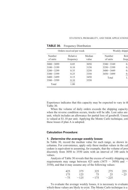
- Page 786 and 787: Statistics, Probability, and Their
- Page 788 and 789: values of X increase by a constant
- Page 790 and 791: 2. Compute the number of possible a
- Page 792 and 793: PROBABILITY OF A SEQUENCE OF EVENTS
- Page 794 and 795: 3 type A units C 5,3. Summing the
- Page 796 and 797: 2. Compute the probability that X
- Page 798 and 799: 2. Find the values of A(z) Let A(zi
- Page 800 and 801: Calculation Procedure: 1. Write the
- Page 802 and 803: The quantity X - is an index of th
- Page 804 and 805: ecomes P(1.841 < < 1.871) 0.95. T
- Page 806 and 807: according to whether the true value
- Page 808 and 809: STATISTICS, PROBABILITY, AND THEIR
- Page 810 and 811: two components, C 1 and C 2, and le
- Page 812 and 813: CORRESPONDENCE BETWEEN POISSON FAIL
- Page 814 and 815: that the system will be operating a
- Page 816 and 817: A composite system may be regarded
- Page 818 and 819: Alternatively, find the number of p
- Page 820 and 821: FIGURE 34 STATISTICS, PROBABILITY,
- Page 822 and 823: Alternatively, find the values of P
- Page 826 and 827: STATISTICS, PROBABILITY, AND THEIR
- Page 828 and 829: Since e 2 is to have a minimum valu
- Page 830 and 831: Calculation Procedure: STATISTICS,
- Page 832 and 833: constitute the steady-state conditi
- Page 834 and 835: ENGINEERING ECONOMICS B_1 BIBLIOGRA
- Page 836 and 837: ENGINEERING ECONOMICS B_3 Materials
- Page 838 and 839: ENGINEERING ECONOMICS B_5 ogy for S
- Page 840 and 841: in steel beam column, 1.110 in brac
- Page 842 and 843: theorem of three moments, 1.63 timb
- Page 844 and 845: ioventing, 4.43, 4.44 combined reme
- Page 846 and 847: specific speed of, 6.74 impellers,
- Page 848 and 849: y ultimate-strength method, 2.32 to
- Page 850 and 851: straight-line, 9.14, 9.15, 9.30 sum
- Page 852 and 853: sum-of-the-digits, 9.20 taxes and e
- Page 854 and 855: Fatigue loading, 1.108 Field astron
- Page 856 and 857: Hanger, steel, 1.166 Head (pumps an
- Page 858 and 859: in small generating sites, 6.84 to
- Page 860 and 861: Member(s): 1.40 to 1.54 axial, desi
- Page 862 and 863: Parabolic arc, 2.75 to 2.78, 5.25 t
- Page 864 and 865: “green” products and, 4.36 hydr
- Page 866 and 867: Prismoidal method for earthwork, 5.
- Page 868 and 869: ENGINEERING ECONOMICS I_16 Pump(s)
- Page 870 and 871: ENGINEERING ECONOMICS I_17 Reciproc
- Page 872 and 873: ENGINEERING ECONOMICS I_18 Scale of
- Page 874 and 875:
ENGINEERING ECONOMICS I_19 Soil: co
- Page 876 and 877:
ENGINEERING ECONOMICS I_20 Steel co
- Page 878 and 879:
ENGINEERING ECONOMICS I_21 Structur
- Page 880 and 881:
ENGINEERING ECONOMICS I_22 Turbines
- Page 882 and 883:
ENGINEERING ECONOMICS I_23 Water-su