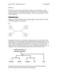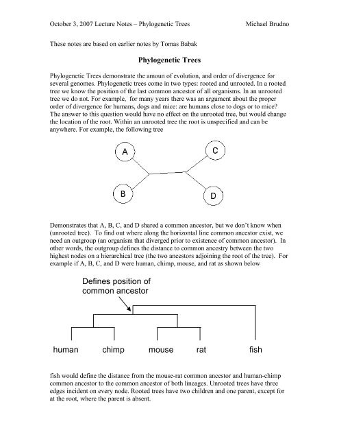
human chimp mouse fish rat Defines position of common ancestor

October 3, 2007 Lecture Notes – Phylogenetic Trees Michael Brudno
These notes are based on earlier notes by Tomas Babak
Phylogenetic Trees
Phylogenetic Trees demonstrate the amoun of evolution, and order of divergence for
several genomes. Phylogenetic trees come in two types: rooted and unrooted. In a rooted
tree we know the position of the last common ancestor of all organisms. In an unrooted
tree we do not. For example, for many years there was an argument about the proper
order of divergence for humans, dogs and mice: are humans close to dogs or to mice?
The answer to this question would have no effect on the unrooted tree, but would change
the location of the root. Within an unrooted tree the root is unspecified and can be
anywhere. For example, the following tree
Demonstrates that A, B, C, and D shared a common ancestor, but we don’t know when
(unrooted tree). To find out where along the horizontal line common ancestor exist, we
need an outgroup (an organism that diverged prior to existence of common ancestor). In
other words, the outgroup defines the distance to common ancestry between the two
highest nodes on a hierarchical tree (the two ancestors adjoining the root of the tree). For
example if A, B, C, and D were human, chimp, mouse, and rat as shown below
Defines position of
common ancestor
human chimp mouse rat
fish
fish would define the distance from the mouse-rat common ancestor and human-chimp
common ancestor to the common ancestor of both lineages. Unrooted trees have three
edges incident on every node. Rooted trees have two children and one parent, except for
at the root, where the parent is absent.

October 3, 2007 Lecture Notes – Phylogenetic Trees Michael Brudno
Building Trees
There are two types of approaches to building trees: (i) Distance based methods, which
work from pairwise distances between the sequences (e.g. UPGMA, Neighbour Joining),
(ii) character-based methods, which work directly from multiply aligned sequences (e.g.
parsimony and likelihood approaches). While character-based methods are more
accurate, they are also more complicated, and beyond the scope of the class. However it
is notable that most phylogeny inference packages (e.g. PAML) use these.
Distance-based approaches are also important because they represent a type of algorithm
that w will see many times throughout this class – clustering. In particular the UPGMA
approach we will discuss next is a classical example of hierarchical clustering.
UPGMA
A straightforward method to draw a tree is a greedy approach called the Unweighted Pair
Group Method using Arithmetic Averages (UPGMA). A tree is drawn by recursively
joining two closest nodes, grouping them into one cluster, and treating them as single
node to which new distances are calculated. This is done until only two nodes remain.
Suppose you are given four sequences separated by the following distances:
A
B 4
A B C D
C 5 8
D 7 9 7
To construct the tree we begin with a star tree, where the initial branch point is arbitrary.
A
B
C
D

October 3, 2007 Lecture Notes – Phylogenetic Trees Michael Brudno
A and B are the closest so let’s group them under a new node called F and calculate the
distances to the new node:
The distance from C to F can be calculated as:
d(
C,
B)
+ d(
C,
A)
! d(
A,
B)
d(
C,
F)
=
2
You divide by 2 because you covered the path from C to F twice. The distance matrix
then becomes:
F
C 4.5
F C D
D 6 7
F and C are now closest, repeating the procedure by grouping C and F into G produces
the following tree:
N.B. This is still an unrooted tree as we do not know when C and D diverged.
Neighbor Joining
A
B
A
B
F
F G
C
UPGMA produces the correct tree when the mutation rates along all branches are equal,
however, this is not always the case. Consider the following phylogenetic tree (known to
be correct):
D
C
D

October 3, 2007 Lecture Notes – Phylogenetic Trees Michael Brudno
(http://www.icp.ucl.ac.be/~opperd/private/neighbor.html)
In this case B diverged more quickly than A. Thus, UPGMA would join A and C
producing an incorrect tree topology. Neighbour Joining (NJ) was developed to take
non-uniform divergence rates into account. The idea is to produce a modified distance
matrix that takes into account the net divergence rate of the entire tree, so that nodes
close together but far apart from all other nodes are not necessarily joined directly.
Saitou and Nei (1987) derived a model for calculating the modified matrix. If d is the
original distance matrix, the modified matrix
D ij = dij
! ( Ri
+ R j )
where,
1
R i = dim.
N # 2
!
m"
N
N is the set of leaves in the tree. The number of leaves is | N |. The tree topology is
constructed as described above (UPGMA) using the modified distance matrix D. Atteson
(1999) proved this model to be correct under the assumption that the we are dealing with
an additive tree (i.e. for any two leaves the distance between them is the sum of edges
along a path that connects them).
Suppose you have the following distance matrix d (corresponding to the above tree):
,

October 3, 2007 Lecture Notes – Phylogenetic Trees Michael Brudno
Ri, the net divergence matrix for each sequence is calculated as the sum of each node to
all other nodes.
R(A) = (5+4+7+6+8)/4 = 30/4,
R(B) = 42/4,
R(C) = 32/4,
R(D) = 38/4,
R(E) = 34/4,
R(F) = 44/4.
D is:
It is now apparent that D and E, and A and B are closest and these are initially joined as
neighbours.
Sample calculation for Dij:
D
D
D
D
ij
AB
AB
AB
= d
ij
= d
! ( R + R
AB
! ( R
A
30 42
= 5 ! ( + )
4 4
= ! 13
i
j
)
+ R
B
)
We can now use the greedy algorithm to construct the tree. We would start by joining A
and B (AB->S), since this is one of the minima of D (we could have also joined D and E,
the other minimum), and recompute the distances to S (nodes joining AB; see figure
below).

October 3, 2007 Lecture Notes – Phylogenetic Trees Michael Brudno
B
A
C
Subbing in S for A and B, we can calculate the distances from the remaining nodes to S,
d(CS) = d(AC) + d(BC) - d(AB) / 2 = 3
d(DS) = d(AD) + d(BD) - d(AB) / 2 = 6
d(ES) = d(AE) + d(BE) - d(AB) / 2 = 5
d(FS) = d(AF) + d(BF) - d(AB) / 2 = 7
d becomes:
S C D E F
S
C 3
D 6 7
E 5 6 5
F 7 8 9 8
Where D is:
S C D E F
S
C -19.5
D -18 -18.5
E -17.5 -18 -20.5
F -19.5 -20 -19 -20
We would next join D and E -> T.
F
D
E
B
A
C
S
F
D
E

October 3, 2007 Lecture Notes – Phylogenetic Trees Michael Brudno
B
A
C
S
F
D
E
We would continue to join nodes, recalculate d and D until only two nodes remain.
B
A
C
S
F
T
D
E