Multifractality of US Dollar/Deutsche Mark Exchange Rates - Studies2

More documents

Recommendations

Info

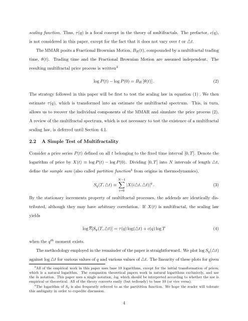
scaling function. Thus, τ(q) is a focal concept in the theory of multifractals. The prefactor, c(q), is not considered in this paper, except for the fact that it does not vary over t or △t. The MMAR posits a Fractional Brownian Motion, BH(t), compounded by a multifractal trading time, θ(t). Trading time and the Fractional Brownian Motion are assumed independent. The resulting multifractal price process is written 3 log P (t) − log P (0) = BH [θ(t)] . (2) The strategy followed in this paper will be first to test the scaling law in equation (1) . We then estimate τ(q), which is transformed into an estimate the multifractal spectrum. This, in turn, allows us to recover the individual components of the MMAR and simulate the price process (2). A review of the multifractal spectrum, which is not necessary to test the existence of a multifractal scaling law, is deferred until Section 4.1. 2.2 A Simple Test of Multifractality Consider a price series P (t) definedonallt belonging to the fixed time interval [0,T]. Denote the logarithm of price by X(t) ≡ log P (t) − log P (0). Dividing [0,T]intoN intervals of length △t, define the sample sum (also called partition function 4 from origins in thermodynamics), Sq(T,△t) ≡ N−1 i=0 |X(i△t, △t)| q . (3) By the stationary increments property of multifractal processes, the addends are identically dis- tributed, although they may have arbitrary correlation. If X(t) is multifractal, the scaling law yields when the q th moment exists. log E[Sq (T,△t)] = τ(q)log(△t)+c(q)logT (4) The methodology employed in the remainder of the paper is straightforward. We plot log Sq(△t) against log △t for various values of q and various values of △t. The linearity of these plots for given 3 All of the empirical work in this paper uses base 10 logarithms, except for the initial transformation of prices, which is a natural logarithm. The companion theoretical papers work in natural logarithms exclusively, and use the ln notation. This paper uses a single notation, log, which should be interpreted according to whether the use is empirical or theoretical. All of the theory converts easily (but tediously) to base 10 (or vice versa). 4 The logarithm of Sq is also frequently referred to as the partitition function. We hope the reader will tolerate this ambiguity in order to expedite discussion. 4
values of q is proposed as a test of the MMAR. We check linearity by visual inspection. The slope of the lines, estimated by OLS regression, gives an estimate of the scaling function τ(q). The estimated scaling function is easily transformed into an estimated multifractal spectrum. Despite the simplicity of these methods, theoretical justification beyond equation (4) is quite difficult. Mandelbrot (1995, Section 6.4) has conjectured consistency of estimated slopes for a large class of multifractals as △t → 0. In general, a theoretical proof of this conjecture has been elusive, except for a few simple cases such as the binomial and multinomial multiplicative cascades. Consistency, along with inference methods, remains an open and interesting area for future theoretical work. Until additional theory is developed, we justify the above methodology on two counts. First, while inversion of logarithms and expectations will produce small sample biases in estimation, these need not prevent transmission of linearity in (4) to approximate linearity in the sample partition function. 5 Secondly, estimation biases for τ(q) can be studied and understood for particular cases of interest. Monte Carlo simulation validates the empirical methods used in this paper. After Section 3 shows linearity in DM/USD partition functions, Section 5 estimates τ(q) and uses this information to generate an estimated multifractal spectrum. Using results provided in MFC and CFM, we then recover a generating mechanism with theoretical multifractal spectrum similar to the data. Simulated partition functions of this process follow their predicted paths, with (approximately) linear partition functions of (approximately) the same slope as the DM/USD data. Finally, the partition function methodology has some power to discriminate against reasonable alternatives. Section 5 simulates GARCH and FIGARCH processes with parameters from pub- lished research on exchange rates. Although the simulated alternatives mimic scaling behavior in individual samples, the MMAR replicates the scaling behavior found in the data more consistently. All of the simulation results should be considered preliminary investigations, and should be studied more thoroughly in future research. 5 By Jensen’s inequality, rewriting equation (4) as a regression yields errors with negative expectation. The effect on linearity of the partition function and estimated slope depends on both the magnitude of the bias and how the bias varies with △t. Both of these problems are tractable with simulation methods, although beyond the scope of the present paper. 5
Page 1 and 2: Multifractality of Deutschemark/ US
Page 3 and 4: 1 Introduction Multifractality is a
Page 5: comprehensive empirical work using
Page 9 and 10: decay rate in autocorrelations of 2
Page 11 and 12: trading time as the cumulative dist
Page 13 and 14: 6 at about two hours. For the remai
Page 15 and 16: empirical work in Section 5. The co
Page 17 and 18: negative fractal dimension will typ
Page 19 and 20: • α0 denotes the value of α for
Page 21 and 22: values of q can be expected to be l
Page 23 and 24: Section 6 shows that SEAS2, used to
Page 25 and 26: H is estimated by equation (6), whi
Page 27 and 28: 6 GARCH and FIGARCH Alternatives Th
Page 29 and 30: their distribution is usually speci
Page 31 and 32: 7.2 Consistency in Subsamples We sp
Page 33 and 34: This last figure is a vignette, rep
Page 35 and 36: 9 Appendix 9.1 Goal of Seasonal Adj
Page 37 and 38: the two series FED1 and FED2. The t
Page 39 and 40: [17] Ghysels, E., On the Economics

Multifractality of US Dollar/Deutsche Mark Exchange Rates - Studies2

Create successful ePaper yourself

Delete template?

Save as template?