Mathematical Modeling and Simulation for Production of MTBE

Ministry of Higher Education
And Scientific Research
University of Technology
Chemical Engineering Department
MATHEMATICAL MODELING AND
SIMULATION FOR PRODUCTION OF MTBE
BY REACTIVE DISTILLATION
A Thesis
Submitted To The
Department of Chemical Engineering of the University of
Technology in a Partial Fulfillment of the Requirements for the
Degree of Master of Science in Chemical Engineering
By
Mohammed Z. Mohammed
B.Sc. in Chemical Engineering, 2003
Supervised by
Dr. Zaidoon M. Shakoor
February / 2009

ﻰﻟﺇ ﺔﻣﺪﻘﻣ ﺓﺡﻭﺮﻁﺍ
ﺕﺎﺒﻠﻄﺘﻣ ﻦﻣ ءﺰﺟ ﻲﻫﻭ ﺔﻴﺟﻮﻟﻮﻨﻜﺘﻟﺍ ﺔﻌﻣﺎﺠﻟﺍ / ﺔﻳﻭﺎﻴﻤﻴﻜﻟﺍ ﺔﺳﺪﻨﻬﻟﺍ ﻢﺴﻗ
ﺔﻳﻭﺎﻴﻤﻴﻜﻟﺍ ﺔﺳﺪﻨﻬﻟﺍ ﻡﻮﻠﻋ ﻲﻓ ﺮﻴﺘﺴﺟﺎﻤﻟﺍ ﺔﺟﺭﺩ ﻞﻴﻧ
ﻞﺒﻗ ﻦﻣ
ﺪﻤﺤﻣ ﻞﻣﺍﺯ ﺪﻤﺤﻣ
( 2003 ﺱﻮﻳﺭﻮﻟﺍﻚﺑ
)
ﺭﻮﺘﻛﺪﻟﺍ ﻑﺍﺮﺷﺈﺑ
ﺭﻮﻜﺷ ﻦﺴﺤﻣ ﻥﻭﺪﻳﺯ
2009 / ﻁﺎﺒﺷ
ﻲﻤﻠﻌﻟ ﺚﺤﺒﻟا و ﻲﻟﺎﻌﻟا
ﺔﻴﺟﻮﻟﻮﻨﻜﺘﻟا ﺔﻌﻣﺎﺠﻟا
ﻢﻴﻠﻌﺘﻟا ةرازو
ﺔﻳوﺎﻴﻤﻴﻜﻟا
ﺔﺳﺪﻨﻬﻟا ﻢﺴﻗ
ﻲﺛﻼﺛ ﻞﻴﺜﻣ ﺝﺎﺘﻧﻹ ﺓﺎﻛﺎﺤﻤﻟﺍﻭ ﻲﺿﺎﻳﺮﻟﺍ ﻞﻳﺩﻮﻤﻟﺍ
ﻲﻠﻋﺎﻔﺘﻟﺍ
ﺮﻴﻄﻘﺘﻟﺍ ﺔﻄﺳﺍﻮﺑ ﺮﺜﻳﺍ ﻞﻴﺗﻮﻴﺑ

ﻪـﻠﻟﺍ ﻢﺴﺑ
ﻢﻴﺣﺮﻟﺍ ﻦﻤﺣﺮﻟﺍ
ﻪـﻠﻟﺍ ﻊﻓﺮﻳ
ﺍﻮﻨﻣﺍ ﻦﻳﺬﻟﺍ
ﻦﻳﺬﻟﺍﻭ ﻢﻜﻨﻣ
ﻢﻠﻌﻟﺍ ﺍﻮﺗﻭﺃ
ﻪـﻠﻟﺍﻭ ﺕﺎﺟﺭﺩ
ﻥﻮﻠﻤﻌﺗ ﺎﻤﺑ
ــــــــــــﻴﺒﺧ
ﺭ

ﺔﻟﺩﺎﺠﻤﻟﺍ
ﻪــﻠﻟﺍ ﻕﺪﺻ
ﻢﻴﻈﻌﻟﺍ

Dedicated to
My father and my mother.
My wife, daughter, and my son.
My brothers and sisters
My supervisor
All my friends
Mohammed

Acknowledgment
Praise be to Allah Who gave me ability to achieve this research.
I wish to express my sincere gratitude, appreciation and
thankfulness to my supervisor. Dr. Zaidoon M. Shakoor for his
kind supervision and continuous advice during the research.
My deep thanks go to Dr. Jamal M. Ali, The Active Head of
Chemical Engineering Department, for his encouragement and
providing facilities through out this work, to thank Dr. Nidhal M.
Al-Azzawi for her assistance.
I wish to thank Dr .Khalid A. Sukker for his assistance.
I would also like to express my acknowledgment to the staff of
Chemical Engineering Department of the University of
Technology. Also great thanks are extended to the staff of the
Central Library in the University.
To all that helped me in one way or another, I wish to express
my thanks.
And finally my special thanks go to my wife for her support
and encouragement.
I
Mohammed

Certificate of Supervisor
I certify that this thesis has been concluded under my supervision in a
partial fulfillment of the requirements for the Degree of Master of Science in
Chemical Engineering at the Chemical Engineering Department, University
of Technology.
Signature:
Name:
Date: / 3/ 2009
(Supervisor)
In view of the available recommendations, I forward this thesis for
debate by the Examining Committee.
Signature:
Name: Dr. Khalid A. Sukkar
Assistant Professor Head of Post
Graduate Committee Department of
Chemical Engineering
Date: / 3/ 2009

Certificate of Examiners
We certify, as an Examining Committee, that we have read this thesis
entitled " Mathematical Modeling and Simulation for Production of MTBE
by Reactive Distillation ", examined the student Mohammed Z. Mohammed
in its content and found that the thesis meets the standard for the degree of
Master of Science in Chemical Engineering.
Signature:
Name: Dr. Zaidoon M. Shakoor
Data: / 3/ 2009
(supervisor)
Signature:
Name: Assistant Professor Dr. Mohammed F. Abed
Data: / 3 / 2009
(Member)
Signature:
Name Assistant Professor Dr. Shada A. Samih
Data: / / 2009
(Member)
Signature:
Name: Dr. Abbas H. Slaimon
Data: /3/ 2009
(Chairman)
Approved by the Acting Head of the Chemical Engineering Department
Signature:
Name: Dr. Jamal M. Ali
Head of Chemical Engineering Department
Data: / 3 / 2009

Certification
I certify that this thesis entitled (Mathematical Modeling and
Simulation for Production of MTBE by Reactive Distillation) was prepared
under my linguistic supervision. It was amended to meet the style of English
Language.
Signature:
Name: Eyad Shamselden
Date: / 3/ 2009

ABSTRACT
In this thesis, theoretical investigations have been made concerning reactive
distillation columns. The detailed steady state modeling, and simulation are made
for two important oxygenates produced by reactive distillation columns, they are
methyl tertiary butyl ether (MTBE) and ethyl tertiary butyl ether(ETBE).
This study was performed through several steps in order to construct and develop
an improved steady state model based
on recent manner of MESH equations ( Mass balance, Equilibrium, Summation
of composition, and Heat balance) the reaction portion added to the mass and
energy balance.
This model was developed to study the behavior of multi component non
ideal mixture in reactive distillation. The set of algebraic equations governing
steady state composition profile in a reactive distillation column are solved by
using Gausses elimination method.
The developed model can be employed to simulate the reactive distillation
operation. This model required the in advance specification of number of reactive
and non-reactive trays, the reflux ratio, composition and flow rates of the feed,
and heat duty to determine the result of the following:
• The liquid and vapor composition profiles.
• The temperature profile.
• The top product (distillate) flow rate, temperature, and composition.
• The bottom product (reboiler) flow rate, temperature, and composition.
• The reaction profiles for reactive trays.
An analysis is performed in order to show the impact on the reactive
separation system by adding or subtracting either non-reactive or reactive
separation stages, keeping constant number of total stages, and other variables
such as feed ratio, catalyst weight per tray, location of feed, and reflux ratio.
II

In the MTBE case study, when reflux ratio equal to seven, 1100kg of catalyst
per tray, 8 reactive trays, and 10 th and 11 th
isobutene lead to get the best purity, yield, and conversion.
The validity of the developed steady state equilibrium model had been
evaluated by comparing its predictions with another theoretical work.
III
feed locations for methanol and
The residue curve map(RCM) plotted for the system that do not react then
for reactive system, these non reactive RCM and reactive RCM have studied for
both oxygenates (MTBE, and ETBE).
The calculations and simulations in this thesis were obtained by using
MATLAB environment, version 7.
This simulation model can be adapted to any reactive distillation application.

Contents
IV
Contents
Page No.
Acknowledgment .......................................................................................... I
Abstract ........................................................................................................ II
Contents ..................................................................................................... IV
Nomenclature ............................................................................................ VIII
Greek Symbols ............................................................................................ IX
List of Abbreviations ................................................................................... X
Chapter One: Introduction
1.1 Introduction .............................................................................................. 1
1.2 Separation process ................................................................................... 1
1.3 Reactive distillation simulation ............................................................... 3
1.4 Residue curve map ................................................................................... 3
1.5 Scope of the present work ........................................................................ 4
Chapter Two: Literature Survey
2.1 Introduction ............................................................................................. 5
2.2 Application of reactive distillation .......................................................... 7
2.3 Advantages and constraints ...................................................................... 9
2.3.1 The advantages ...................................................................................... 9
2.3.2 The constraints .................................................................................... 14

V
Contents
2.4 The stage models. ................................................................................. 16
2.4.1 The equilibrium model....................................................................... 20
2.4.2 Non equilibrium or Rate-Based Model .............................................. 23
2.4.3 Comparison of equilibrium and non equilibrium models................. 25
2.5. Gasoline additives (Oxygenates) ......................................................... 29
2.5.1 Methyl tertiary butyl ether .................................................................. 29
2.5.2 Ethyl tertiary butyl ether ..................................................................... 30
2.6 VLE for multi-component distillation .................................................. 31
2.6.1 Thermodynamic models ..................................................................... 32
2.6.2 Ideal vapor liquid equilibrium ............................................................ 33
2.6.3 Non ideal vapor liquid equilibrium ..................................................... 34
2.6.4 Calculation of activity coefficient ...................................................... 34
2.6. 4.1 Wilson model,1962 ......................................................................... 35
2.6.4.2 NRTL model ,1986 .......................................................................... 35
2.6.4.3 UNIQUAC model,1975 .......................................................................... 35
2.6.4.4 UNIFAC Model,1975 ............................................................................. 36
2.7 Residue curve map (RCM) .................................................................. 38
2.7.1 Residue curve map plot ..................................................................... 41
2.7.2 Distillation regions and boundaries ................................................... 43
2.7.3 Residue curve map with reaction (kinetically controlled) ................ 43
Chapter Three: Modeling & Simulation
3.1 Introduction ............................................................................................ 46
3.2 Steady state modeling of continuous packed RD column ..................... 47

VI
Contents
3.2.1 Model assumptions ....................................................................... 47
3.2.2 Estimation of model parameters ................................................... 48
3.2.2.a. Equilibrium relations ................................................... 48
3.2.2.b. Antoine model ............................................................. 49
3.2.2.c. Bubble point calculation ............................................ 49
3.2.2.d Enthalpy estimation ..................................................... 50
3.3 Steady State Model equations ................................................................ 52
3.3.1 Non reactive trays ......................................................................... 52
3.3.2 Reactive trays ................................................................................ 53
3.3.3 Condenser ..................................................................................... 53
3.3.4 Reboiler ......................................................................................... 54
3.4 Degree of freedom ............................................................................... 55
3.5 Case studies .......................................................................................... 57
3.5.1 Case study one .............................................................................. 57
3.5.2 Case study two .............................................................................. 59
3.6 Simulation by MATLAB ....................................................................... 62
Chapter Four: Results and Discussion
4.1 Introduction ............................................................................................ 64
4.2 Model validity ........................................................................................ 64
4.3 Effect of reactive tray change ................................................................ 68
4.4 Effect of Variation of Feed Location ..................................................... 71
4.5 Effect of feed ratio ................................................................................. 72

VII
Contents
4.6 Catalyst effects ............................................................................. 74
4.7 Effect of reflux ratio ......................................................................... 75
4.8 General effects investigation for ETBE case study ........................ 85
4.9 Non reacting residue curve map ...................................................... 89
4.10 Kinetically controlled residue curve map ...................................... 92
Chapter Five: Conclusions and Recommendations
5.1 Conclusions .......................................................................................... 100
5.2 Recommendations for Future Work .................................................... 101
References
Appendixes
Appendix (A): Sample of Calculation of Real Enthalpy
Appendix (B): Physical Properties of Pure Components
Appendix (C): Activity Coefficient Models
Appendix (D): Model Data
Appendix (E): Results of Models

Nomenclature
Symbol Definition Units
A, B,
and C
Antoine’s coefficient [−]
A , B ,
and C
Ideal vapor enthalpy coefficient [−]
a Activity [−]
a
ij
a ,b , c ,
and d
Non-temperature dependent energy parameter
between components i and j
VIII
[J/mol]
enthalpy coefficient [−]
bij Temperature dependent energy parameter
between components i and j
[J/mol. k]
c Number of component [−]
Cp Specific heat of a component [kJ/kg. ْ◌ C]
Da Damkohler number ( H rref. /V) [−]
2
Ð Maxwell Stefan diffusivity [mP P/s]
D Distillate flow rate [ mol/hr]
F Feed molar flow rate [mol/hr]
f Fugacity [pa]
h Liquid phase enthalpy [J/mol]
H Vapor phase enthalpy [J/mol]
H molar holdup [ mol/hr]
I Component identification number [-]
J Stage identification number [-]
K thermodynamic equilibrium coefficient
[−]
L 1BMolar flow rate of liquid [mol/hr]
m Material balance summation [mol]
Mwi Molecular weight of component i [mol/kg]
N Interfacial mass transfer [mol/hr]
Number of components of a mixture
[−]
NC
n
Pt
Number of trays
Total pressure [pa]
[−]

Symbol Definition Units
Pi
Q
R
vapor pressure of pure component [pa]
Rate of heat transfer [Watt]
Universal gas constant [J/mol. K ]
Rr Dimensionless reaction rate (r/rref). [- ]
RR
Reflux ratio [- ]
r Reaction rate [mol/s]
S
Side stream mole flow rate [mol/hr]
T Temperature [k]
t 2Btime hr
V 3BMolar flow rate of vapor [mol/hr]
X Liquid phase mole fraction [−]
Y Vapor phase mole fraction [−]
Subscript Symbols
Symbol Definition
av Average value
B Bottom product
C Condenser
c Critical value
D Distillate product
F Feed
i Component i
Li Component i in liquid phase
Vi Component i in vapor phase
j Tray
n Segment (stage) index
IX

Greek Symbols
Symbol Definition Units
α Vapor activity coefficient [ _ ]
γ Liquid activity coefficient [ _ ]
ΔE The error [ o C]
ε Reaction volume [m 3 ]
ξ Time dimensionless [−]
λ Latent heat [J/mole]
Λ Parameter in Wilson model [−]
υ Stoechiometric coefficient of component [−]
ρ Density [kg/m 3 ]
Φ Fugacity coefficient [−]
List of Abbreviations
Symbol Definition
EFAO Europe Fuel Associated Organization
EQ Equilibrium
ETBE Ethyl tertiary butyl ether
IB Isobutene
MATLAB Matrix Laboratory
MESH (Material balance, Equilibrium, Summation of mole, Heat balance)
MTBE Methyl tertiary butyl ether
NB Normal butane
NEQ Non equilibrium
RCM Residue curve map
RD Reactive distillation
TAME Tertiary amyl methyl ether
VLE Vapor Liquid Equilibrium
X

Chapter One Introduction
1.1 INTRODUCTION:
Chapter One
Introduction
Distillation is the most important separation method in refinery and
chemical industry. In terms of installed capacity and energy usage, the
commitment of the process industry to this unit operation is enormous. In USA,
for example, the energy consumed by distillation is equivelent to about 7.5 % of
the U.S. oil consumption (Kimmo, 1998). Reactive distillation (RD) is a
combination of separation and reaction in a single vessel, the combination of
reaction and distillation is an old idea that has received renewed attention
recently. There are two main types of reactive distillation, batch and continuous,
the continuous RD is largerly used for production scale, constant product
composition, and continuous feed provision.
1.2 SEPARATION PROCESS:
The driving force for any distillation process is the difference between the
liquid and vapor composition in the mixture. When the liquid and the vapor have
the same composition at a certain point, this mixture is called azeotropic mixture
and this point is called azeotropic point. Therefore there is no driving force for
separation at this point, and the azeotropic mixtures cannot be separated by
conventional distillation technique.
The conventional distillation can produce azeotropic products, which must
be separated by using other methods. There are several enhanced distillation
methods which can be used to separate azeotropic mixtures, such as
(Perry,1997; Seader, 2006) :
1

Chapter One Introduction
1. Pressure swing distillation.
2. Salted distillation.
3. Extractive distillation.
4. Azeotropic distillation.
5. Reactive distillation.
As shown above the presence of the azeotrope in a mixture makes
separation by conventional distillation difficult. Azeotropes can form distillation
regions, which limit the separation. When reacive distillation process is used,
improvements can be obtained by really integrating the tasks, on the following
items:
• On the reaction: because there is an equilibrium displacement, since the
products are being withdrawn.
• On the separation: because of the changes in the driving force for mass
transfer due to the reaction.
There are several applications of reactive distillation to separate azeotropic
mixtures in industry, for example production of octane boosters (MTBE,
TAME, and ETBE)
2

Chapter One Introduction
1.3 REACTIVE DISTILLATION SIMULATION:
The design and operation issues for reactive distillation (RD) system are
considerably more complex than those involved for either conventional reactor
or conventional distillation column. The introduction of an in-situ separation
function within the reaction zone leads to complex interactions between vapor-
liquid equilibrium, vapor-liquid mass transfer, intra-catalyst diffusion (for
heterogeneously catalyzed process) and chemical kinetics. Such interactions
have been shown to lead to the phenomenon of multiple and complex dynamics
which have been verified in experimental laboratory and pilot plant unit (Isao,
1971). Although rigorous design of this column by NEQ stage model is carried
out by Baur and Krishna, 2000 the effect of various parameters by continuation
analysis has not been investigated for this column configuration. Mathematical
optimization methods are generally very powerful for generating and evaluating
design alternatives.
1.4
Residue curve is the locus of the liquid composition X (t) remaining at
any given time in the still. Residue curve map is a collection of liquid residue
curves originating from different initial composition.
Residue curves and residue curve maps have been extensively studied for
over 100 years. Much of the literature in this field deals with systems that do not
react. Chemical reactions can influence residue curve maps in some important
ways(Ross T., et. al., 2006). For example, it is known that reactions can lead to
both the appearance and disappearance of stationary points (azeotropes), and
that reactive azeotropes can exist even in systems that otherwise would be
considered thermodynamically ideal. It follows that chemical reactions can
influence the very existence of separation boundaries and, therefore, the design
and synthesis of reactive separation processes. Examples of such systems
3

Chapter One Introduction
include four-component systems with a single reaction and quarterly systems
with a kinetically controlled reaction which are taken for ETBE and MTBE.
1.5 SCOPE OF THIS WORK:
The main objectives of the present study include the following:
1. Studying the feasibility of the reactive distillation due to study of the non
reacting residue curve map and then with reaction for two oxygenates methyl
tertiary butyl ether (MTBE) and ethyl tertiary butyl ether (ETBE).
2. Development of a steady state model for the reactive distillation of MTBE
and ETBE.
3. Establishment developed and generalized program to solve the model
equations which can be used as a basis for reactive distillation design
concepts, by performing the mass and energy balances around the reactive
distillation column.
4. Studying the effects of process variables, and selection of the best values of
variables of MTBE and ETBE produced by reactive distillation.
RESIDUE CURVE MAP:
4

Chapter Two Literature Survey
2.1 INTRODUCTION:
Chapter Two
Literature Survey
In recent years, increasing attention has been directed towards reactive
distillation process as alternative to conventional processes (reactor and then
separation). This has led to development of a variety of techniques for reactive
multistage column; however, in 2005 Cristhain investigated the conceptual of
reactive distillation (RD) process and an attempt is made with this design
strategy to conjugate the strengths of graphical and optimization-based method.
The authors analyzed several methods available in design and operation, and
they suggested some guidelines to propose a reactive distillation process. These
guidelines are separated in levels, and the first level is the feasibility analysis.
Certainly the first important task before the proposition of a feasible separation
scheme is to study the system behavior.
The potential benefits of applying RD processes are taxed by significant
complexities in process development and design. For reactions that are
irreversible, it is more economical to take the reaction to completion in a reactor
and then separate the products in a separate distillation column (Harvey, 2004).
The principles may be illustrated when we look for an example process for the
production of chemical C out of A and B according the following reaction
scheme:
A + B ↔ C + D
(2.1)
In addition some undesired side reactions are assumed, such as for example:
A+ C ↔ E
(2.2)
5

Chapter Two Literature Survey
2 C ↔ F
(2.3)
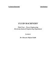
This reaction can be carried out in a conventional process setup as
sketched on the left side of Figure (2.1), the objective is to produce C out of
reactants A and B, thereby making byproduct D. In addition, there are undesired
side and consecutive reactions, so that the exit stream of the reactor will be a
mixture of all components.
A and B have to be separated and recycled, C has to be separated and
purified to separation, and D, E, and F have to be disposed of. Normally, this
will require more than the single distillation column that is given in Figure (2.1).
Shown on the right hand side of Figure (2.1) is a typical setup for reactive
distillation column. The reactions will take place in the reactive section.
Figure 2.1 Schematic representation of a conventional
and reactive distillation process(Around, 1999)
6

Chapter Two Literature Survey
In case of a heterogeneous reaction, this section can consist of reactive packing
elements but also of trays that are covered with a teabag type. For homogeneous
reactions, the location of the reactive section is defined by the feed location of a
homogeneous liquid catalyst. The non-reactive rectifying and stripping section
take care of additional product separation. In this kind of setup there is in-situ
product removal of desired product C, which will pull the equilibrium of the
main reaction towards the right hand side, thereby increasing the overall
conversion. This way one can overcome a bad equilibrium constant. In addition,
lowering the concentration of C due to the in-situ separation will also reduce the
rates of side reactions, there will be less conversion of C to undesired side
products, and this illustrates how reactive distillation may be applied to systems
where selectivity is important.
The non-reactive section in the column play an important role in product
separation and reactants recycle. In the ideal case, the non-reactive zones
separate the products from the reactant in such away that the reactants are
automatically flushed back into the reactive zone, while pure products may be
obtained as product stream. The design and operation issues for reactive
distillation (RD) system are considerable more complex than those involved for
either conventional reactor or conventional distillation column.
2.2 APPLICATION OF REACTIVE DISTILLATION:
There are a large number of processes that have been proposed for
reactive distillation (Doherty et. al., 1992; Kai, et. al., 2002), but only very few
found industrial application. There are various reasons for the lack of
application, the most important of which is that most companies are reluctant to
try something that has been never done before and will rather use proven
technology. In addition, since in reactive distillation all is done in one vessel, the
7

Chapter Two Literature Survey
possibilities for control are fairly limited, if a design is, therefore, not optimized
before it is built. The most important application of reactive distillation is the
production of fuel ethers because the success of the MTBE process was boosted
by phase out of lead based anti-knock agents in gasoline. These octane
enhancers are nowadays mainly replaced by MTBE or similar oxygenates like
ethyl tertiary butyl ether (ETBE) and tertiary amyl methyl ether (TAME). For
some time, MTBE has been the fastest growing chemical (Ainsworth, 1991), and
over the last two decade a considerable number of plants for production of these
oxygenate were built, many based on reactive distillation technology.
The concept of combining these two important functions for enhancement
of overall performance is not new in the chemical engineering world. The
recovery of ammonia in the Solvay process from soda ash of the 1860s may be
cited as probably the first commercial application of reactive distillation (Kai, et.
al., 2002). Many old processes have made use of this concept. The production of
propylene oxide, ethylene dichloride, sodium methoxide, and various esters of
carboxylic acids are some examples of processes in which RD has found a place
in some form or another, without attracting attention to a different class of
operation. It was not until the 1980s, when the enormous demand for MTBE
(methyl tertiary butyl ether), that the process gained separate status as a
promising multifunctional reactor and separator. Table (2-1) represent a
different benefits of industrial important reactions either implemented on
commercial scale or have been investigated on laboratory scale, using Reactive
Distillation.
8

Chapter Two Literature Survey
Table (2.1) Examples of reactive distillation
Reaction The benefit References
methanol + isobutene ↔MTBE To enhance the conversion Baur et.al. , 2000
of isobutene, achieve Around,1999
separation if i-C4 from
Cristhain.P,2008
C4 stream and, decrease or
eliminate side reaction
ethanol +isobutene ↔ETBE
acetaldehyde +acetic anhydride
↔vinyl acetate
benzene + propylene ↔cumene
To utilize bio-ethanol and
surpass equilibrium
conversion
To improve safe process
with high purity.
To use of exothermic of
reaction, high purity
cumene, and for much
cheaper.
n-paraffin ↔ iso-paraffin To increase the octane
value of paraffin stock
methanol from synthesis gas For better temperature
control and improve yield
methanol /dimethyl ether+ CO
↔ acetic acid
Hexamethylene diamine + adipic
acid ↔nylon 6, 6 prepolymer
Production of high purity
acetic acid
To enhance the conversion
and good quality polymer
2.3 ADVANTGES AND CONSTRAINTS.
2.3.1 The Advantages:
9
Al-Arfaj M. A. et.
al., 2002
EFAO, 2006
Zoeller J.R. ,et.
al.,1998
Kai et. al., 2002
Lebas E.,et. al.
1999
Watanbe R., et.
al. 1997
Kai, et. al., 2002
Doherty M.F., et.
al. 1987
The advantages and constraints in reactive distillation are specific to each
system. The advantages of reactive distillation in general are:
1. Chemical equilibrium limitation can be overcome, an equilibrium reaction
can be driven to completion by separation of products from the reacting
mixture (i.e., reaction conversion can approach 100%). Higher conversions
are obtained due to shifting of the equilibrium to the right. This is

Chapter Two Literature Survey
exemplified by the production of methyl acetate. ( Stankiewicz, 2003; Agreda
et. al., 1990) and tertiary amyl ether (Bravo et. al., 1993).
2. Higher selectivity can be achieved, elimination of possible side reaction by
removal of the product from the reaction zone. This can serve to increase
selectivity. In some applications particularly in cases when thermodynamic
reaction prevents high conversion the coupling of distillation to remove
reaction product from reaction zone can improve the overall conversion and
selectivity significantly, for example in the production of propylene oxide
from propylene chlorohydrins (Carra et. al., 1979 ) and for alkylation of
benzene to produce cumene (Shoemaker and Jones, 1987).
3. Improvement quantity of used materials. For example, it may be possible to
operate with a reduction in the amount of excess reactant fed to the reactor.
Normally feeding one reactant in excess is used to shift the equilibrium
towards the production of product. With reactive distillation, this shift is
attained through removal of the reaction products from reaction phase. Also
elimination by-product formation may allow the use of lesser quantities of
reactant. It may also be possible to avoid auxiliary solvent. In the production
of MTBE, in industrial practice when conventional reactor used, a 10%
excess of methanol is used in order to reduce mainly isobutylene dimmers
by-product formation. (Elkanzi E. M, 1995). The excess of methanol causes
some problems in separating the product MTBE from non reacted reactant,
because MTBE forms azeotropes with methanol and i-C4. The separation task
is therefore difficult. While MTBE is obtained with high purity from feed
equimolar quantities of methanol and i-C4 when reactive distillation is used,
because this scheme allows for "reacting away" the azeotropes (Taylor R. and
Krishna ,2000). Figurers (2.2) and (2.3) show MTBE production by reactive
distillation and conventional distillation respectively.
10

Chapter Two Literature Survey
Figure(2-2) Processing schemes for the etherification reaction
MeOH +
IB ↔ MTBE
11

Chapter Two Literature Survey
12
Figure(2-3) Conventional route for the synthesis of MTBE: two stage MTBE process: R01: tubula
reactor; R02-R03: adiabatic reactors; HX: heat exchanger; M: mixer; D: divider; S01-S02: distillation
towers (adapted from Peters et al. (2000)).

Chapter Two Literature Survey
4. The heat of reaction can be used in-situ for distillation, saving associated
energy costs, through use of energy released by exothermic reaction for
vaporization. This reduces the reboiler heat duty which is supplied normally
by steam. Benefits of heat integration are obtained because the heat generated
in chemical reaction is used for vaporization, this particularly advantageous
for situation involving heat of reaction such the hydration of ethylene oxide
(Circ et. al., 1994).
5. Reduction of hotspot, because the liquid vaporization provides a sink for
thermal energy. This is beneficial in, for example, the hydrolysis of ethylene
oxide to ethylene glycol (Ciric et. al.,1994).
Increasing process efficiently and reducing of investment and operational
cost are direct result of this approach (Cristhain, et. al., 2008).
Effecting distillation and reaction simultaneously reduces the capital cost
and includes benefits such as reduction of recycle, optimization of separation,
lower requirements of pump, instrument and piping.
The most spectacular is in production of methyl acetate, the traditional
process uses one reactor and nine distillation columns (Taylor R. and Krishna,
2000). When reactive distillation is used, only one reactive distillation column is
needed. The conventional and reactive distillation of methyl acetate are shown in
Figure (2.4.a) and Figure (2.4.b) respectively.
13

Chapter Two Literature Survey
Figure(2-4) Processing schemes for the esterification reaction
MeOH + AcOH ↔ MeOAc + H 2O
(a) conventional processing scheme consisting of one reactor followed by
nine distillation columns. (b) the reactive distillation configuration
(Taylor R. and Krishna R., 1985).
2.3.2 The Constraints:
The constraints on using reactive distillation are:
1. Reactive distillation is not suitable for every process where reaction and
separation steps occur. Operating conditions, such as pressure and
temperature of reactive and separation process and perhaps other
requirement, must overlap in order to assure the feasibility of combined
process. In some processing the optimum conditions of temperature and
pressure for distillation may be far from optimal condition for reaction and
vice versa. This limitation can be overcome by fixing adequate operating
conditions in the cases where this is possible.
14

Chapter Two Literature Survey
2. Suitable volatilities of reactants and products to keep high concentration of
reactant in reaction zone (Seader, 2006) gives three cases ideal for reactive
distillation.
i. A R or A 2R , R is more volatile than A
ii. A R or A 2R , A is more volatile than R
iii. 2A R+S or A+B R+S, A and B are intermediate in
volatility to R and S, R is the most volatile
3. Reaction may form "reactive azeotropes ". these azeotropes are included by
the reaction affecting the separation.
4. Difficulties in providing proper residence time characteristics. If the residence
time for the reaction is long, it may require a large column size and a large
hold-up leading to the process becoming uneconomical compared with
standard separate reactor and distillation column setup (Neil E Small, 2004).
5. Scale up to large flows. It is difficult to design RD process for very large flow
rates because of liquid distribution problems in packed RD columns.
6. Although RD process intensification allows for saving cost, in return, control
issues are more complex than conventional schemes are.
7. A very stable catalyst is required for heterogeneous system. Catalyst
deactivation may have a marked effect on column performance and is not
easily overcome.
However, some of above the limitations may be circumvented by using reactive
extraction instead of reactive distillation.
15

Chapter Two Literature Survey
2.4 THE STAGE MODELS:
A reactive distillation problem can be studied using different approaches
including: feasibility, simulation, modeling, design and experimental studies in
the laboratory and the pilot plant. A combination of all of these methods gives
rise to the most accurate solution to the problem. One very important aspect of
predicting the behavior in these systems is the model used to design and simulate
the reactive distillation process. An effective way of decomposing the modeling
aspects of reactive distillation involves the following classification of the models
existing for distillation with reaction (Baur, 2000):
I. Steady-state equilibrium stage model.
II. Dynamic equilibrium stage model.
III. Steady-state non-equilibrium stage model;
IV. Dynamic non-equilibrium stage model;
V. Steady-state non-equilibrium cell model, that accounts for staging of the
vapor and liquid phases inside the column.
Two primary approaches available in the literature for modeling reactive
distillation columns will be taken up .
I. Equilibrium stage model.
II. Non-equilibrium stage model.
Much more popular have been the models incorporating phase equilibrium,
while taking into account finite reaction rates. (Nelson,1971; Suzuki et al.,1971;
Carra et al. 1979; Alejski et al. 1988; Chang and Seader, 1988; Aljeski, et al.
1991; Simandl and svrecek,1991; Ciric and Gu, 1994; Abufares and Douglas,
1995; Perez-Cesneros et al.,1997). The models presented in all of these papers
are more or less the same.
They incorporate a set of liquid and vapor mass balances along with
equilibrium correlations for the vapor liquid equilibrium calculation. The
reaction is normally tackled by implement a kinetics expression into the liquid
16

Chapter Two Literature Survey
phase overall mass balance and the liquid phase composition balances. The
above models vary mainly in the way the equations are solved, or objectives of
the model. The models presented by Nelson (1971) and Suzuki et al., (1971) are
extensions of numerical methods originally developed for normal distillation.
Nelson uses a Newton Raphson method for solving the model equations. Suzuki
uses Muller's method. Carra et al., (1979) also use Newton method for solving
the model equations. They use their model for steady state simulation of un
experimental column for the production of propylene oxide from chloro hydrins.
Alejski (1991) presents a model for taking into account liquid phase plug
flow on a distillation tray. This is done by modeling the liquid phase on a tray as
a cascade of mixing cells. The model was solved with a Newton Raphson
algorithm.
Chang and Seader (1988) present a model along with a homotopy method
for solving the model equations. Homotopy methods are generally more robust
and have much wider range of convergence than Newton method. Calculations
times for the Homotopy method are, however, much higher than for that
Newton's method.
Simandl and Svrcek (1991) present a model along with two different
solution methods the first method is a simultaneous solution method after
linearization of the equations. The second one is inside-outside algorithm. The
latter was found to converge much faster than the simultaneous method, and the
robustness was found to be similar.
In (Jacob and Krishna, 1993). For MTBE synthesis using the column
configuration, shown in Figure (2.5), varying the location of the stage to which
methanol is feed results. When methanol is fed to stages 10 or 11, steady state
multiplicity is observed (Baur, et. al., 2000)
17

Chapter Two Literature Survey
Figure (2.5) Configuration of the MTBE synthesis column, following
Jacobs and Krishna (1993), the bottom flow is fixed at 203 mol/s
Ciric and Gu (1994) present a somewhat different approach. They directly
implemented the equations for capitalized and variable cost into the model
equations. The resulting mixed integer nonlinear programming (MINLP) model
determines the optimal configuration and operating conditions.
Abufares and Douglas (1995) present a steady state and a dynamic model
describing a reactive distillation. They use the ASPEN PLUS RADFRAC with a
standard equilibrium stage column model that may be extended to take into
account chemical reactions (Venkataraman et. al, 1990).
RADFRAC is used by Jacobs and Krishna 1993, Nijhuis et al. ,1993 and
Hauan et al., 1995.
18

Chapter Two Literature Survey
Sneesby et al. (1997a) uses both PRO / II and ASPEN PLUS for steady state
modeling of a column for production of ETBE. In their second paper ( Sneesby
et al., 1997b), they present a dynamic model, which they solve with SPEED UP
dynamic simulator.
A somewhat different approach to the equilibrium model is presented by
Perez-Cisneros et al., (1997). Their model uses so called "elements" rather than
the actual components. The chemical elements are the molecule parts that remain
invariant during the reaction, and the actual molecules may be formed by
different combinations of elements. The benefit of this approach is that chemical
and physical equilibrium problems in reactive mixture are the same as a strictly
physical equilibrium model. The method however is unsuitable for extension to
non equilibrium models because the real components are required for transfer
rate calculations rather than the chemical elements.
Non-equilibrium models belong to more recent times. The first work in
this field was presented by Sawistowski et al., (1979) who modeled a packed
reactive distillation column for esterification of methanol and acetic acid to
methyl acetate. They used an effective diffusivity method for their mass transfer
model. Fourier's law was used for heat transfer modeling. The resulting system
of differential equations was solved using a Runge-kutta method.
Higler, et al., 1999 developed a generic NEQ model for packed distillation
column. The important features of the model are the use of Maxwell Stefan
equation for description of intra phase mass transfer and incorporation of a
homotopy like continuation method that allows for easy tracking of multiple
steady state.
Jianjum, et al., 2003 developed the dynamic rate-based and equilibrium
model for packed reactive distillation column. The dynamic responses of
controlled variables ( product purity and reactant conversion) to a step change in
manipulated variables (reflux ratio, bottom rate, and reboiler duty) were studied
19

Chapter Two Literature Survey
with both the dynamic and equilibrium model. The dynamic response of reactant
conversion is very non-linear unconventional, but the response of product purity
is well approximated by linear first order differential equation.
Reactive distillation of ETBE production was performed by Young et al.
2003, from their study, the internal profiles of RD process especially total reflux
operation, can be well understood, which is almost impossible in actual process.
And efforts are devoted to explain the observed results in physical aspect.
Calculation algorithm is based on Luyben algorithm, and rigorous energy
balance is used with vapor flow rate calculation by iteration. Internal profiles of
RD column for both total reflux and process after this are observed and analyzed
in the simulation tool MATLAB.
Antti Pyhälahti , 2005 studied the setting up a reactive distillation process
for production of TAME, the results of this study has a significant impact on the
development of the highly successful NExTAME and NExETHERS
technologies, even if the final solution is based on the Side Reactor Concept
(SRC).
The technical re-conversion of MTBE process to produce ETBE was
studied by (Isela, et al. 2007) using a non equilibrium model in reactive
distillation with an UNIFAC method at steady state. The simulation was carried
out in Aspen Plus, analyzing the possibility of using actual instillation of MTBE
plant as it works, to produce ETBE. The analysis of azeotrope condition revealed
that the ethanol-to-isobutene molar feed ratio is the main factor affecting the
equilibrium.
2.4.1 The Equilibrium Model:
The equilibrium stage model assumes that the vapor and liquid stream
leaving a given stage are in thermodynamic equilibrium with one another
(Krishna and Taylor, 1985). A schematic diagram of an equilibrium stage is
20

Chapter Two Literature Survey
shown in Figure (2.6). Vapor from the stage below and liquid from the stage
above are brought in to contact on stage together with any fresh or recycle feeds,
the vapor and liquid streams leaving the stage are assumed to be in equilibrium
with each other.
Figure (2.6): General Equilibrium Stage Model, Including
Feed Stage and Side Stream Product Withdrawal.
The equations on the equilibrium stage model are also known as MESH
being acronym:
• The M equations are the material balance equations.
• The E equations are phase equilibrium relations.
• The S equations are summation equations.
• The H equations are heat (enthalpy) equation.
21

Chapter Two Literature Survey
dm
dt
j
= L
j−
1
+ V
j+
1
+ F
j
− S
v
j
−V
j
− L
j
− S
l
j
+
r c
∑∑ υ i,
j R i,
mε
j
(2.4)
m=
1 i=
1
dm j xi,
j
v l r c
= L
j−1
x
i,
j−1
+ V
j+
1
y
i,
j+
1
+ Fj
zi,
j − ( S j + V j ) yi,
j − ( L j + S j ) xi,
j + ∑ ∑ i,
j
dt
m=
1i= 1
22
υ R (2.5)
i,
mε
j
y
i,
j k x
i,
j i,
j
= (2.6)
1
1 , = ∑ c
X (2.7)
i=
i j
c
∑
i=
1
y 1
(2.8)
i,
j =
dH j xi,
j
v v l l
= L
j−1
h
i,
j−1
+ V
j+
1
H
i,
j+
1
+ F j H − ( S j + V j ) H i j − ( L j + S j ) h + Q
dt
j
,
j j
The (mj) is the hold-up on the stage j. With very few exceptions, mj
(2.9)
considered to be the hold-up only of the liquid, it is, however, important to
include the hold up of vapor phase at higher pressure. The last term in equations
r c
(2.4 to 2.5) ( ∑ ∑ νi
Ri m j
m=
1i= 1
, j , ε ) is the rate of the disappearance of the total
moles due to any m reaction of the stage j. Equation (2.5) is the component
material balance (neglecting the vapor hold-up), vi, m represents the
stocheometric coefficient of component i in reaction m and εj
reaction volume.
The E equations are phase equilibrium relations, the compositions of the
stream leaving stage are in thermodynamic equilibrium. Therefore, the mole
is
represents the

Chapter Two Literature Survey
fractions of component i in the liquid and vapor streams leaving stage j by the
equilibrium relationship are shown in equation (2.6).
The S equation are summation equations (2.7 and 2.8) are two equations
arise from the necessity that mole fraction of all components, in either liquid or
vapor phase, sum to unity .
The enthalpy balance is given by equation (2.9), the left side represents
the accumulation of enthalpy on stage. It represents the total enthalpy of stage,
but for the reason given above this will normally be the liquid phase enthalpy.
At steady state condition, all terms per time equal to zero.
Some authors include additional equation in their (mostly unsteady state )
models, for example pressure drop, controller equations, and so on.
2.4.2 Non Equilibrium or Rate-Based Model (NEQ Model).
A non-equilibrium (NEQ) or rate-based model employs a transport
phenomenon approach and the film model description for predicting the mass
transfer rates. It assumes equilibrium is established at the interface between
vapor and liquid phases. The model equation for a generic stage j (The NEQ
stage may represent a tray or section of packing column) and component i may
be represented based on conventional distillation equation that incorporate the
chemical reaction term (Taylor and Krishna ,1985). A schematic representation
of the NEQ stage is shown in Figure (2.7).
V
L
j+
1
j−1
The component molar balance for the vapor and liquid phases is
y
x
i,
j+
1
i,
j−1
−
−
V
L
j
j
x
y
i,
j
i,
j
+
+
f
f
l
v
j,
j
j,
j
−
−
N
N
v
i,
j
l
i,
j
= 0
= 0
NRi,jR are the interfacial mass transfer rates, at the vapor-liquid interface.
23
(2.10)
(2.11)

Chapter Two Literature Survey
|
P PRI R(2-12)R
L
The continuity equation
The enthalpy balances for both vapor and liquid phases are
V
R
24
R R(2.13)R
R
N
l |
P PRI i =
R
N
v
i
(2.14)R
ERj Ris the interface energy transfer rates, the product of the energy fluxes and the
net interfacial area.
|
j−1
The continuity of the energy transfer rates at the interface is
P PR R (2-15)R
y
RT
R E
l |
P PRI i =
NRi,j Ris usually obtained from the Maxwell-Stefan equation for mass transfer in
multi-component system. The Maxwell-Stefan equations from mass transfer in
the vapor and liquid respectively are given by
i
v
j+
1
H
H
l
j−1
v
j+
1
−
−
L
V
j
j
H
H
l
j
v
j
+
+
H
v
v
∂μ
c y −
i
i N k yk
N
= ∑ v v
∂z
k = 1 ct
Di,
k
f
l
j
f
v
j
H
lf
j
v
i
.)
x
RT
i
l
= 0
l
l
l
∂μ
c −
i xi
N k yk
N i
= ∑ l l
∂z
k = 1 ct
Di,
k
R R(2-16)
RE v
i
(2-17)
NRi Ris molar fluxes of species i , and the ÐRi,kR represent the corresponding
Maxwell Stefan diffusivity of the i-k pair in appropriate phase. The energy flux
is related to conductivity and convection as follows
vf
j
−
−
E
E
l
j
+
v
j
−
Q
Q
l
j
v
j
= 0

Chapter Two Literature Survey
E
∂T
l
l l
= − j λ j
c l
+ ∑i=
1 N i,
j
l
(2-18)
i,
j
∂η
H
Figure (2.7): General Non Equilibrium Stage Model, Including
Feed Stage and Side Stream Product Withdrawal.
2.4.3 Comparison of Equilibrium (EQ) and Non Equilibrium
(NEQ) Models.
1. For EQ model, only the number of stages and two physical properties (vapor
liquid equilibrium and enthalpies) are needed, While the NEQ model requires
thermodynamic properties, not only for calculation of phase equilibrium but
also for calculation of driving forces for mass transfer and, in reactive
distillation, for taking into account the effect of non-ideal component
25

Chapter Two Literature Survey
behavior in the calculation of reaction rates and chemical equilibrium
coefficient, in addition to physical properties such as surface tension,
diffusion coefficient, viscosities, etc. for calculation of mass (and heat)
transfer coefficient and interfacial area. Table (2.2) shows the properties that
needed for EQ and NEQ in a models Ibrahim, S.S.,2007.
Table (2.2) the needed properties for EQ and NEQ models
Non-Equilibrium Model
26
Equilibrium Model
Activity Coefficients Activity Coefficients
Vapor Pressures Vapor Pressures
Fugacity Coefficients Fugacity Coefficients
Densities Densities
Enthalpies Enthalpies
Diffusivities
Viscosities
Surface Tension
Thermal Conductivities
Mass-Transfer Coefficients
Heat-Transfer Coefficients
2. Solving the rate-based model is always much more difficult than solving the
equilibrium model for all of the simulations. The EQ model can be solved
first, and the results can be used as the initial guess for the rate-based
model.
3. The drawback of EQ model is the evaluation of the efficiencies for the plate
or HETP for the packing column in the case of multi component reactive
mixture. Pouzineau, et al. compare between the two models by studying

Chapter Two Literature Survey
Acetic anhydride reaction with water to obtain two moles of Acetic Acid,
the prediction of EQ model was equivalent to the NEQ model.
Baur et al., 2000 developed a generic NEQ cell model for RD tray
columns of production of ethylene glycol, they concluded that the dynamic EQ
model, widely used in the literature, shows much less sensitivity to disturbance,
that is important in case of studying control concept , but studying of effect of
various parameters, gives in many cases nearly the same results
Jianjun, 2004 et al. compare between a steady-state equilibrium and rate-
based models for packed reactive distillation columns for the production of
tertiary amyl methyl ether (TAME) and methyl acetate.
They concluded that the number of equations in the rate-based model is 5-7
times the number of equations in the equilibrium model if the number of
segments in the rate-based model is the same as the number of theoretical stages
in the equilibrium model. For example at same number of segments. For methyl
acetate no. of equation for EQ is 407 while for NEQ is 1899, and For TAME
no. of equation for EQ was 600 while for NEQ was 4430. An optimal reflux
ratio and an optimal operating pressure were found for both the TAME system
and the methyl acetate system. The optimal values predicted by the equilibrium
model and the rate-based model are very close. Also the mole fraction profile
for the two cases in Figure (2.8)
27

Chapter Two Literature Survey
(a) (b)
28
( c )
( c ) ( d )
Figure (2.8) Comparison of temperature and composition profiles between the
equilibrium model and rate based model (a,b) for the methyl acetate system
(c,d) for the TAME system ( Jianjun et al. 2004),.

Chapter Two Literature Survey
2.5 GASOLINE ADDITIVES (OXYGENATES)
Oxygenates are compounds containing oxygen in a chain of carbon and
hydrogen atoms. Today, oxygenates are blended into gasoline in two forms:
alcohols or ethers. When added to gasoline, alcohols by themselves tend to be
very volatile, formation of an azeotrope with light hydrocarbons, and water
soluble, which can create problems in the fuel distribution system and vehicle
engine as well as in the environment. These problems of volatility and water
solubility can be overcome by "stabilizing" the alcohols with various petroleum-
derived components through a process known as etherification. Ethers retain all
the benefits of their alcohol feedstock, without their shortcomings,
(EFOA,2006). Ternary ethyl lead is still used in Iraq as a gasoline additive for
octane booster, this component causes massive environmental pollution. MTBE,
TAME, or ETBE units could be established for producing high octane gasoline
and reducing the pollution, especially the raw material of most of these ethers
can found in many refinery units such as cracking.
2.5.1 Methyl Tertiary Butyl Ether.
MTBE is almost exclusively used as a fuel component in motor gasoline,
MTBE is also produced in huge amounts as anti-knock agent in gasoline, where
it has replaced tetraethyl lead to large extent (Marceglia and Oriani ,1982 ).
Moreover, MTBE has become the second largest volume organic chemical
produced in U.S. after ethylene (Raisch,1994). Therefore the production of
MTBE by reactive distillation is of great industrial importance (Smith and
Huddleston,1982; Tadé, Datta and Smith ,1997). The production of Methyl Tert-
butyl ether is presented using a reactive distillation column in order to convert
methanol and isobutene for obtaining MTBE, according to the reaction.
CH
3
OH
i
C
H
+ − 4 8
↔
MTBE
29

Chapter Two Literature Survey
N-butene is presented in the feed mixture but it is inert for the reaction, for
the conventional reactor-separator scheme, methanol is usually fed in excess in
order to improve the conversion of i-C4 into MTBE. This causes some problems
for separating the product MTBE from the non reacted reactants because MTBE
forms azeotropes with methanol and i-C4. The separation task is difficult. In this
work, it is proposed to feed equimolar quantities of methanol and i-C4
stoichiometric proportion, and product with high purity of MTBE is obtain.
Thus, the problem of splitting azeotropic mixture is reduced because the reactive
distillation scheme allows for "reacting away" the azeotropes (Taylor and
Krishna, 2000)
2.5.2 Ethyl Tertiary Butyl Ether
30
, in
The production of ethyl tertiary butyl ether is presented using a reactive
distillation column in order to convert ethanol and isobutene for obtaining
ETBE, according to the reversible reaction over an acidic catalyst, such as the
acidic ion-exchanger resin Amberlyst 15.
C
2
H
6
O
i
C
H
+ − 4 8
↔
ETBE
ETBE is produced via reactive distillation by either feeding a single
partially reacted mixture to the column or by feeding two fresh reactant streams
directly to the column at different feed tray locations. The hydrocarbon feed is
obtained from an upstream unit in the refinery (fluidized catalytic cracker, steam
cracker, isobutene dehydrogenation unit, etc.). In any of these units the butane
product contains isobutene, normal butane, and other light hydrocarbons.
Therefore, the butane feed to the column contains large amounts of inert, which
go out from the top of the column because they are much lighter than the product
ETBE. The ethanol fresh feed is usually essentially pure to minimize side
reactions.

Chapter Two Literature Survey
The performance of a packed column is often expressed in terms of the
height equivalence to a theoretical plate (HETP). The HETP is related to the
height of packing by
H
HETP = ( 2.
19)
N
eqm
where Neqm
is the number of equilibrium stages needed to accomplish the
same separation possible in a real packed column of height H. Although the
theory of distillation is well known, the estimation methods for efficiencies are
still relatively inaccurate. The factors that affect efficiencies can be divided into
three groups: the structural, functional, and the system factors and physical
properties. To the best of our knowledge there are no fundamentally sound
methods for estimating either efficiency or HETPs in RD operations(Taylor and
Krishna, 2000) .
2.6 VAPOR LIQUID EQUILIBRIUM FOR MULTI-COMPONENT
DISTILLATION.
For multi-component mixture, graphical representation of properties,
cannot be used to determine equilibrium-stage requirements. Analytical
computation procedures must be applied with thermodynamic properties
depending on temperature, pressure and phase composition, these equations tend
to be complex. Nevertheless the equations are widely used for computing phase
equilibrium ratios ( K-values), enthalpies and densities of mixture over a wide
range of conditions. Vapor liquid equilibrium calculations are usually carried out
for separation processes with several versions. The prediction of mixture vapor
liquid equilibrium is more complicated than prediction of pure component.
Phase equilibrium relation is one of the fundamental properties which are
necessary for the separation processes, and useful equation have been proposed
31

Chapter Two Literature Survey
for expressing relation. Efficient design of distillation equipment requires
quantitative understanding of vapor liquid equilibria in multi component mixture
as expressed through vapor phase fugacity coefficient and liquid phase activity
coefficients.
2.6.1 Thermodynamic models
To describe the phase equilibrium of a system of NC components at a
temperature T and pressure P, the vapor phase fugacity is equal to the liquid
phase fugacity for every component.
∧ v
f i
=
∧ l
f i
i=1, 2, 3. . . . . NC
The vapor phase fugacity can be written in terms of the vapor phase
fugacity coefficient
∧ v
i
∧
i
f = y Φi
P
∧
i
Φ ; vapor mole fraction y i ; and total pressure P as follows.
Also the liquid phase fugacity can be written in terms of liquid phase
32
(2.20)
activity coefficient γ i ; liquid mole fraction x i ; and liquid phase properties f i as
follows.
∧
l
i
f = x γ f
where
i
i
i
fi is calculated using the equation:
sat ( P P ) ⎤
i
⎥
⎥
(2.21)
⎡ l
sat sat Vi
−
fi
= Φi
Pi
exp ⎢
(2.22)
⎢⎣
RT ⎦
At equilibrium
sat
iPi
xi
yi
=
Φ P
γ
where
i
Φ i is given by the equation;
(2.23)

Chapter Two Literature Survey
Φ ∧
i
= Φ
∧
sat ( P P ) ⎤
i
⎥
⎥
Φ ⎡
i Vi
−
Φi
= exp ⎢−
(2.24)
sat
Φi
⎢⎣
RT ⎦
At low pressures, vapor phases usually approximate ideal gases for which
sat
i
= 1
and Poynthing factor which is represented by the exponential differs
from unity by only a few parts per thusand. Therefore equation (2.19) is written
as.
sat
iPi
yi = ⋅ x
P
γ
t
i
2.6.2 Ideal Vapor Liquid Equilibrium
33
(2.25)
Vapor liquid equilibrium is one of the most important fundamental
properties in simulation, optimization and design of any distillation process.
The mixture is called ideal if both liquid and vapor are ideal mixtures of
sat
ideal components, thus in the vapor phase the partial pressure of component P i
is proportional to its mole fraction in the vapor phase according to Daltons law.
sat
i = y P
(2.26)
P i
The equilibrium relationship for any component is defined as.
y
i K = (2.27)
xi
For ideal mixture the K value can be predicted from Raoult’s law, where.
.
K
y
x
i
=
i
sat
Pi
P
= (2.28)

Chapter Two Literature Survey
2.6.3 Non Ideal Vapor Liquid Equilibrium
For non-ideal mixture or azeotropic mixture additional variable γ i (activity
coefficient) appears in vapor-liquid equilibrium equation.
sat
iPi
yi = ⋅ xi
P
γ
t
where γ i represents degree of deviation from reality.
34
(2.30)
when γ = 1,the
mixture is said to be ideal which simplifies the equation to
i
Raoult’s law. For non-ideal mixture γ ≠ 1,
exhibits either positive deviation
from Raoult’s law ( γ > 1),
or negative deviation from Raoult’s law ( γ < 1).
i
2.6.4 Calculation of Activity Coefficient.
i
The prediction of liquid phase activity coefficient is most important for
design calculation of non-ideal distillation. Before calculating vapor-liquid
equilibrium of non-ideal mixture, the activity coefficient of each component
must be calculated.
There are several excess energy (gP
E
P)P
Pmodels to calculate the activity
coefficient for multicomponent systems, the most important models are of
(Wilson, NRTL, UNIFAC, and UNIQUAC). In all these models, the model
parameters are determined by fitting the experimental data of binary mixtures.
Each one of these models has advantages and disadvantages. There is no general
model which has a good representation of all azeotropic mixtures. The selection
of appropriate model for a given mixture is based on three characteristics, which
are temperature, pressure and composition. If inappropriate model is selected,
the design and simulation of the process will not work well.
i

Chapter Two Literature Survey
2.6.4.1 Wilson Model,1962
Wilson and Deal (1962) used the following equation to calculate the liquid
phase activity coefficient.
γ = 1 − ln
i
N
C
∑
j=
1
x
j
Λ
ij
−
N
⎡
⎢
x Λ
C
∑ ⎢ k
NC
K = 1 ⎢
⎢∑
⎣
k = 1
Λ
ki
kj
⎤
⎥
⎥
⎥
⎥
⎦
35
(2.30)
The Wilson model has the disadvantage that it cannot predict vapor liquid
equilibrium when two liquids exist in the liquid phase.
2.6.4.2 NRTL Model, 1986
The NRTL (non-random, two liquid model) was developed by Renon and
Prausnitz (1968). This model uses three binary interaction parameters for each
binary pair in multicomponent mixture-pairs. For NC components system, it
requires N ( −1)
2 molecular binary pair. This equation is applicable to
C N C
multicomponent vapor-liquid, liquid- liquid, and vapor-liquid-liquid systems.
The main equation used to calculate liquid phase activity coefficient for
NRTL model is (SimBasis 2003).
ln
N
C
∑
τ x
C
∑
k = 1
C
∑ NC
j=
1
∑
k = 1
⎛
⎜
C
∑
ji j ji N
mj m mj
j=
1
j ij ⎜ m=
1
γ =
+
−
⎟
i
τ
N
ij
(2.31)
N
x
k
G
G
ki
x
x
G
K
G
kj
⎜
⎜
⎝
N
τ
C
∑
k = 1
The NRTL group interaction parameters are defined in literature (Gmehling
et al. 1977).
2.6.4.3 Uniquac Model,1975
Abrams and Prausnitz (1975) developed the UNIQUAC (UNIversal QUAsi
Chemical) activity coefficient model. This model distinguishes two contributions
termed combinational (C) and residual (R).
x
x
k
G
G
kj
⎞
⎟
⎟
⎟
⎠

Chapter Two Literature Survey
C
i
R
i
ln γ = ln γ ( combinational)
+ ln γ ( residual)
(2.32)
i
The combinational part basically accounts for non-ideality of a mixture
arising from differences in size and shape of constituent molecular species;
whereas the residual part considers the difference between inter-molecular and
intramolecular interaction energies.
The two-parameter UNIQUAC equation gives a good representation of the
vapor-liquid equilibria of binary and multi component mixtures(SimBasis 2003).
c φ z θ φ
lnγ
= ln
x l
(2.33)
i
NC
i
i
i
+ qi
ln + li
− ∑ xi 2 φi
xi
j=
1
j
C
∑ NC
j=
1
∑
k = 1
j
NC
R
lnγ
i = −qi
ln( ∑θ
iτ
ji ) + qi
N
− qi
θ jτ
ij
(2.33)
j=
1
θ τ
Values for parameters are given by Gmehling et al., (1977-1984).
2.6.4.4 Unifac Model,1975
k
kj
Fredensland et al. (1975) describe UNIFAC model (UNIQUAC functional
group model). In UNIFAC model each molecule is taken as a composite of
subgroups; for example t-butanol is composed of 3 "CH3" groups, 1 "C" group
and 1 "OH" group also ethane contains two "CH3"
groups. The interaction
parameters between different molecules are defined in literature.
This model is also called group contribution model, which is based
theoretically on UNIQUAC equation (2.32). The activity coefficient consists of
two parts, combinational and residual contributions.
C
R
lnγ = lnγ
( combinational)
+ lnγ
( residual)
(2.34)
i
i
i
The combinational contribution C
γ i takes into account the effects arising
R
from difference in molecular size and shape while residual contribution γ i takes
36

Chapter Two Literature Survey
into account energetic interactions between the functional group in the mixture.
The combinational part is given by the equation(Smith and Van Ness 1987).
C Φ i li
Φ i
lnγ i = ln + 5qi
ln + li
− ∑ x jl
j
(2.35)
x Φ x
i
The residual contribution is given by.
∑
i
i
j
R
i
i
lnγ υ (lnΓ
− lnΓ
)
(2.36)
i
= K
K
K
⎡
ln ΓK = K ⎢1
− ln( ∑θ
mψ
mK ) −∑
( θ mψ
Km ∑θ
nψ
⎢⎣
m
m n
K
θ (2.37)
Hansen et al. (1991)
1. It has explicit temperature dependence.
37
nm
⎤
) ⎥
⎥⎦
provide a computer aided system for UNIFAC
parameters calculation. UNIFAC model is extensively used to describe
thermodynamics in chemical engineering literature. It is widely used in process
simulation.
2. It has a large library of functional groups from which thousands of
chemicals can be built.
3. It can be updated and expanded, as more experimental data are available.
4. Finally, UNIFAC model can be used when the binary interaction
parameters are not available for other models.

Chapter Two Literature Survey
2.7
RESIDUE CURVE MAP (RCM)
The first step in distillation of azeotropic mixture is the constructing of a
residue curve map for the mixture under consideration. The residue curve map
provides a graphical tool for multi-component azeotropic mixtures prediction if
the feasible separation which could be obtained before any simulation or
experimental study of the distillation process. The residue curve behaves as
batch distillation with single equilibrium stage.
The biggest benefit of residue curve map is that it is a qualitative
description of the composition profile that could be observed in an actual
distillation tower. The residue curve map has the ability to characterize and
distinguish between different ternary systems having azeotropes. The shapes of
the residue curves are very useful in the design of real finite reflux distillation
columns since they give a qualitative picture of the composition profiles in
actual staged distillation columns (Wasylkiewicz et al., 1999a).
To understand the residue curve map, notice Figure (2.9) which represents a
simple residue curve map (Chwan Yee 2003) .
Fig. (2.9) Residue Curve Map and Distillation Boundary
of a Ternary Mixture System (Chwan Yee 2003) .
38

Chapter Two Literature Survey
The residue curve starts at the light pure component region (lowest boiling
temperature), and moves towards the intermediate boiling component, and end at
the heavy pure component in the same region (highest boiling temperature). The
lowest temperature nodes are termed unstable nodes (UN), all trajectories leave
from them; while the highest temperature points in the region are termed stable
nodes (SN), as all trajectories ultimately reach them. These nodes can be either
azeotropes or pure components. The points that the trajectories approach from
one direction and end in a different direction (as always is the point of
intermediate boiling component) are termed saddle points (S).
To determine the relationship between the number of nodes (stable and
unstable) and saddle points necessary in legitimately drawn ternary residue plot
there are several studies in which the equations are based on topological
arguments. The most useful form of these equations is presented by Van Dongen
and Doherty, 1985.
4 3 3
2 2 1 1
( N − S ) + 2(
N − S ) + ( N − S ) = 1
(2.38)
where
N i =number of nodes (stable and unstable) involving i species.
S i =number of saddles involving i species.
Ternary mixtures containing only one azeotrope may exhibit six possible
residue curve maps that differ by the binary pair forming the azeotrope and by
whether the azeotrope is minimum or maximum boiling.
Bernot et al. (1990, 1991) use residue curves in analyzing batch distillation.
They made very interesting work in finding the still and product paths and batch
distillation regions for 3 and 4 component systems. They found the batch
distillation boundaries for any region by joining the unstable node to all the
saddles and nodes of this region. They used the stable separatrices to divide the
39

Chapter Two Literature Survey
composition space. Also they
Pham and Doherty (1990b) recognized that the residue curve map of a
heterogeneous mixture does not differ from that for a homogeneous mixture with
the same set of singular points.
used residue curve maps to select suitable
extractive agents and the sequence of product removal by estimating the
performance of the tower.
Fien and Liu (1994) and Widagdo and Seider (1996) use residue curves as a
standard tool for design of a column.
Safrit et al. (1995)
present residue curve map for continuous distillation of
ternary mixture and they showed that it could be applied to batch distillation at
the current instance of time.
Westerberg and Wahnschafft (1996) put the basis to find the feasibility of
azeotropic distillation by using residue curve map.
Almeida Rivera et. al. (2004) published some perspectives about reactive
distillation processes. The authors have analyzed several methods available for
design and operation, and they suggest some guideline to propose a RD process.
These guidelines are separated in levels, and first level is feasibility analysis.
Certainly, the first important task before the proposition of a feasible separation
scheme is to study the system behavior.
Cristhain p. (2005) have suggested the methods and tools needed for
reactive distillation process synthesis, analysis, and evaluation. The first of these
methods is improved residue curve map technique
40

Chapter Two Literature Survey
According to literature the residue curve map has the following properties
(Doherty and Perkins 1978a)
:
1. The residue curves always point in the direction of increasing temperature.
2. Pure components and azeotropes define fixed points in the map.
3. Azeotropes define boundaries in the composition space, showing different
qualitative behaviors depending on where initial compositions is in the
space.
4. Boundaries define distillation regions, which can not be crossed by simple
stage-by-stage distillation.
5. Residue curves are equivalent to the composition profile, one would get
running a distillation tower at fixed pressure and infinite reflux.
2.7.1 Residue Curve Map Plot
To construct the residue curve map experimentally, a liquid mixture is
charged to the still pot and the pot is differentially heated to produce vapor. The
vapor in equilibrium with the liquid is removed as soon as it forms. The
concentration of the more volatile component is higher in the vapor than in the
equilibrium liquid. With time the concentration of the more volatile component
decreases in liquid and the liquid boiling point increases. The composition of
liquid in still pot versus time produces single residue curve map. By starting
from different initial compositions, different residue curves are formed and the
plot of these curves is called residue curve map.
Using appropriate thermodynamic model, it is easy to construct the residue
curves theoretically without making any experiments. Doherty and Perkins
(1978 a) also Westerberg and Wahnschafft (1996), start with the mole balances
for the batch distillation and generate a set of NC linearly independent,
autonomous, ordinary differential equations, whose solution for various initial
41

Chapter Two Literature Survey
conditions produces a residue curve map. They assume that the still pot is
charged with M(t = 0) moles of a NC
d
dt
( x M ) = x
i
i
dM
dt
dxi
+ M = −yiV
dt
component mixture having a composition
vector X(t = 0). The liquid is differentially heated to form a vapor, which is in
equilibrium with the liquid. The vapor has composition y(x) , is removed the
instant it forms, and has a flowrate V(t).
But
Combining Eqn. (2.39) and (2.40) gives
Where i=1, 2 ….. NC -1 (2.39)
42
dM
(2.40) = −V
dt
dxi
M ( t)
= V ( t)(
xi
− yi
) where i=1, 2 …..NRC R-1 (2.41)
dt
Since the vapor flow V (t) is an arbitrary (positive) function of time then let.
M ( 0)
V ( t)
ξ ( t) = ln( ) = ⋅ t
(2.42)
M ( t)
M ( t)
By substitution for ξ (t)
resulting the final formulation is.
dx
dξ
i = xi
− yi
Where i=1,2 ….. NRCR -1 (2.43)
For different initial still compositions, integration of equation (2.43)
produces several residue curves. From the mathematical point this equation is
non-linear ordinary differential equation, which can be integrated numerically
over the dimensionless time from initial point to final point.

Chapter Two Literature Survey
2.7.2 Distillation Regions and Boundaries
The distillation boundaries are important features of the residue curve map
because they inhibit some separations from being accomplished by ordinary
distillation (Thomas 1991).
The distillation boundaries divide the composition diagram into a number
of distillation regions. The presence of an azeotrope in a multi-component
mixture induces distillation boundaries, which cannot be crossed by simple
distillation.
In batch distillation region any initial distillation composition leads to the
same sequences of cuts. To know the available distillation products for the
studied systems and before any distillation experiments it is important to
investigate the distillation boundaries and regions. The knowledge of batch
distillation boundaries helps us to know if the available separation could be
reached or not. Therefore feasible product regions for any azeotropic must lie
within distillation boundaries. Boundaries between distillation regions cannot be
crossed by using simple distillation.
2.7.3 Residue Curve Map With Reaction
Residue curves and residue curve maps have been extensively studied for
over 100 years(Ostwald,1900; Schreinemakers, 1902 ;Taylor R., 2006). For
mixtures that have azeotrpe, separation boundaries may exist, and these
boundaries are important in separation process synthesis.
Much of the literature in this field deals with systems that do not react.
However, over the last 20 years or so, reactive separations have come in for
considerable attention (Doherty, 2001; Taylor, 2000). Chemical reactions can
influence residue curve maps in some important ways. For example, reactions
43

Chapter Two Literature Survey
can lead to the disappearance of some azeotropes that exist in the absence of
reaction. Chemical reactions can also lead to the creation of new azeotropes that
would not exist in the absence of reaction. Moreover, the reactive azeotropes can
exist even in the system that otherwise would be considered thermodynamically
ideal. It follows that chemical reactions can influence the very existence of
separation boundaries and, therefore, the design and synthesis of reactive
separation processes(Doherty,2001).
The influence of reaction kinetics on chemical phase equilibrium and
reactive azeotrope was investigated first by (Venimadhavan et al. 1994). For a
single reaction, the residue curves are obtained from
dxi
= xi
− yi
+ Da(
υi
− υxi
) Rr
(2.44)
dξ
where Rr =( r/rref)
is a dimensionless reaction rate. Da is the Damkohler
number (a dimensionless measure of the rate of reaction) defined by Da
( H rref/V), where H is the molar holdup and V is the molar flow of vapor
leaving the still. When Da = 0, equation (2-44) simplifies to equation (2-43) for
non-reacting systems. The other extreme of high Da leads to a reaction
equilibrium. For other values of the Damkohler number, equation (2-43) must
be expressed in terms of mole fractions, because for kinetically controlled
systems there is no composition transformation that can lead to the simple form
of reaction equilibrium equation. The stationary points of these equations are
obtained by setting the derivative terms in equation (2-44) to zero. Figures (2-
10) shows the residue curve map for ternary system (IB-MeOH-MTBE) at 11
atm. without reaction. While Figure (2-11) show the same system at 8 atm. with
reaction.
44

Chapter Two Literature Survey
Figure 2.10 Residue curves in the non-reacting ternary system isobutenemethanol-MTBE
at 11 atm. Numbers near residue curves are the lengths of
the corresponding curve, azeotrope. (Taylor R., et. al.,2006).
Figure 2.11 Residue curves in the reacting ternary system isobutenemethanol-MTBE
at 8 atm. Numbers near residue curves are the lengths of the
corresponding curve , azeotrope. (Taylor R. , et. al.,2006).
45

Chapter Three Modeling and simulation
3.1 INTRODUCTION
Chapter Three
Modeling and simulation
A model is a set of assumptions about the operation of the system, logical,
algorithm, and mathematical (Graham Horton, 2001). Mathematical model of
any process is a set of equations including the necessary input data to solve the
equations, whose solution gives a specified data representative of the process to
a corresponding set input, that allows us to predict the behavior of chemical
process system (Wayne 1998,Denn 1986). Processing modeling has made
substantial progress over decades (Pantelides, 2001). Today, computer
simulation is used extensively to analyze the dynamic chemical process or
design controllers and study their effectiveness in controlling the process. The
simulation operations make it possible to evaluate the influence of variables on
any process theoretically. Steady state simulation of parameter system involves
the solution of algebraic equations, while dynamic simulation involves the
solution of ordinary differential equations. Also by comparing the experimental
results with simulation results, one can decide if it is necessary to develop a
more detailed model or it is possible to introduce simplifying assumptions to the
model. The simulation is also used to fix the experimental conditions needed for
design, optimization, and control. Engineers are now capable of building
mathematical models with a degree of details and prediction.
The equilibrium stage model is widely adopted to describe the distillation
process because of its simplicity and convenience. In this chapter, a steady state
model was developed to simulate reactive distillation columns of MTBE and
ETBE production. The set of algebraic equations covering the steady state
composition, vapor flow rates, and liquid flow rates was determined by using
46

Chapter Three Modeling and simulation
matrix method, the temperature profile was determined by using Newton
Raphsin's method. A computer program written by MATLAB environment
(version 7) is used to perform all the calculation. There are many solution
methods for the distillation models to solve different distillation systems,
especially for complex multi component distillation column, these methods have
different applicable occasions (Chen et al, 2004). The selection of solution
method is therefore a very important issue (Taylor and Krishna, 2000).
3.2 STEADY STATE MODELING OF CONTINUOUS PACKED
REACTIVE DISTILLATION COLUMN:
3.2.1 Model Assumptions:
The reactive distillation column is modeled as a tray column, using
reactive and non reactive stages where appropriate. The vapor and liquid stream
leaving a stage are in thermodynamic equilibrium with one another. This is
known as equilibrium model for reactive distillation, the condenser and reboiler
stage numbered 1 and N, respectively. Figure (3-1) represents a scheme of the
reactive tray in continuous reactive distillation column.
The proposed model for reactive distillation column includes the
following assumption:
1. Steady state
2. Neglect of vapor holdup.
3. Column pressure is constant.
4. Perfect mixing on all stages and in all vessels ( condenser and
reboiler)
5. Total condensation.
6. The streams leaving any particular stage are in equilibrium with
each other.
47

Chapter Three Modeling and simulation
7. The condenser and the rebioler are treated as equilibrium stages.
8. The stage efficiency is assumed 100% (for simplicity).
Most of models consider liquid flow rate of output in distillate and bottom
constant, and most often it is esterification reaction. The present model deals
with this flow rates as a variable, and etherification reaction.
y
v n
n Ln− 1x n−1
+ y
n x
vn 1 n+
1
48
L n
Figure (3-1) Scheme of the reactive tray in continuous
reactive distillation column
3.2.2 Estimation Of Model Parameters
a) Equilibrium relations
For non-ideal mixture additional variable γi
of deviation from ideality
K
i
i ⋅ Pi
=
P
γ
appears to represent the degree
(3.1)
The vapor phase is assumed to behave ideally (φ=1) and the liquid phase
for MTBE system (four components system) is modeled using Wilson activity
coefficient equation (Appendix C, table C-1). This method is accurate for multi
component mixture that doesn't form two liquid phases (Kooijman and Taylor,
2000), also UNIFAC activity coefficient model is used for ETBE(Appendix C,
from table C-2 to table C-4).
A+B C

Chapter Three Modeling and simulation
b) Antoine Model:
The vapor pressure of each component in this study is obtained by using
Antoine equation:
ln( P ) = A
B
+
T + C
where the temperature T is in Kevin and pressure in kp
49
( 3.2)
Appendix (B), Table (B-3) contains parameters of Antoine equation for
all component used in this study.
c) Bubble Point Calculation:
The most widely employed numerical method for estimating bubble point
of a mixture is the Newton Raphson's technique. For distillation process the
liquid of each tray is at its bubble point and the vapor above the plate is at its
dew point. The bubble point of multi component mixture and constant
pressure can be calculated by trial and error on the equilibrium relationships
y = k x
( 3.3 )
i
i
i
When liquid at its bubble point then
c
∑ k i xi
i=
1
Error! Bookmark not defined. = 1
( 3.4)
Moreover, when the vapor is at its dew point
Y
i
∑ Ki
= 1
To estimate the bubble point by Newton Raphson's iterative method
equation (3.6) is written in the form
(3.5)
f ( T )
+ 1 = T −
(3.6)
'
f ( T )
Tn n
where

Chapter Three Modeling and simulation
c
f ( T ) Kixi
−1
(3.7)
f
'
= ∑
i=
1
c dK i
( T ) xi
(3.8)
dT
= ∑
i=
1
d) Enthalpy Estimation
Vapor enthalpy is a function of temperature and pressure. The ideal vapor
state enthalpy H* is chosen as a reference, because it depends only on
temperature, and it is identical to the zero pressure enthalpy of real fluid at the
same temperature:
H* (T) = H (T, P = 0) (3.9)
Edmister (1984) expressed the ideal vapor enthalpy, for many hydrocarbons,
as fifth order polynomial:
H*-H*0 = A+BT+CT^2+DT^3+ET^4+FT^5 (3.10)
where; T is in R and H* is in Btu/lb. The constants of the above equation are
listed in Appendix A, Table (A-2) for each component of the system under
consideration.
The reactive distillation column of the MTBE is operating at high pressure,
low temperature, so it is important to estimate the enthalpy of each component at
the related operating pressure, because of the deviation from the ideal vapor
state. Edmister procedure is used to estimate these enthalpies:
H = (H*-H) + (H*- H*0) + H*0
H = enthalpy at T and P
H*-H = enthalpy departure from simple fluid.
H*-H*0 = ideal vapor enthalpy.
H* = ideal vapor enthalpy at T = 0
0
H* 0 is equal to zero at T = 0 for the operating temperature ranges.
50
(3-11)

Chapter Three Modeling and simulation
(H*-H) is found for the operating temperature range and operating pressure of
each distillation column from the following equation:
where;
0
1
H * −H
⎛ H * −H
⎞ ⎛ H * −H
⎞
=
⎜
⎟ + ω ⎜
⎟
(3.12)
RTc
⎝ RTc
⎠ ⎝ RTc
⎠
H * −H
RTc
= enthalpy departure at any temperature and pressure.
0
⎛ H * −H
⎞
⎜
⎟ = enthalpy departure of simple fluid at the temperature and pressure.
⎝ RTc
⎠
1
⎛ H * −H
⎞
⎜
⎟ = enthalpy correction for real fluid at the same temperature and
⎝ RTc
⎠
pressure.
Equation (3-11) is used to get a fifth order polynomial of enthalpy as a
function of temperature at the operating pressure of the column.
H = a + bT + cT 2 + dT 3 + eT 4 + fT 5
In appendix A, Tables (A-3) shows the constants of equation (3-11) for the
column. A sample of calculation for estimating the enthalpy of n-Butane for
temperature range of ( 345-395K) at the pressure of 11 Bar is shown in (A-1).
For vapor mixture, the Vander Walls mixing rule is used:
where; Hi
c
H mv = ∑
i=
1
Y H
i
vi
51
(3.13)
(3.14)
The partial molar enthalpy of component i in liquid mixture may be
expressed as:
is the molar enthalpy of component i in the vapor mixture.
− λ H h (3.15)
Li
= vi
where λ is the latent heat of vaporization and can be predicted from Watson
formula at any temperature, as follows:
0.
38
⎡ Tc
− T ⎤
λ = λb
⎢ ⎥
(3.16)
⎣Tc
− Tb
⎦

Chapter Three Modeling and simulation
where,
λ b
T
T
b
c
:- latent heat at normal boiling point in KJ/Kmol.
:- boiling point in K.
:- critical temperature in K.
T :- temperature in K.
The values λ b, Tb, Tc
for each component of the system are given in Appendix
B Table (B-3). The enthalpy of liquid mixture is estimated using the following
equation:
c
hL = ∑
i=
1
h
Li
X
i
52
(3-17)
The heat of mixing (heat of solution) is ignored in this work (for organic
solutions the heat of mixing is usually small and can be ignored Edmister 1984).
3.3 STEADY STATE MODEL EQUATIONS
3.3.1 Non Reactive Trays
a) Total material balance:
V
V
L + n+
1 L n
− − = 0
(3.18)
n −1
n
b) Component material balance
V
V
L − X
n+
1Y
L X nY
n
+ − − = 0
(3.19 )
n 1 n−1
n+
1 n n
c) Energy balance
h
V
V
L − n−1
n+
1H
L n n H n
h
+ − − = 0
(3.20)
n 1
n+
1 n
d) Phase equilibrium

Chapter Three Modeling and simulation
( T, P,
X ) * φ ( T,
P,
Y)
i
φ =
l
v
Error! Bookmark not defined. X
*
i
Y
(3-21)
e) Summation
c
∑
i=
1
X −1
= 0
(3.22)
n,
i
3.3.2 Reactive Trays
a) Total material balance:
n
L n V − n L − n V = v
n i R
− 1 + 1 ∑ m,
j
i=
1
+ (3.23)
b) Component material balance:
V
L − X
n+
1Y
L X nY
i n,
i R j
V
+ − − −
= 0
n 1 n−1
n+
1 n n
n ε (3.24)
m,
c) Energy balance:
L + − − −
= 0
−1 h −1
V + 1H
+ 1 L h V H w R , ∆H
(3.25)
n n n n n n n n n n i R
d) Phase equilibrium:
l
v
Error! Bookmark not defined. X =
*
i
Y
(3.26)
e) Summation:
c
∑
i=
1
53
w
i
φ ( T, P,
X ) * φ ( T,
P,
Y)
i
X −1
= 0
(3.27)
n,
i
3.3.3 Condenser
i
i
i

Chapter Three Modeling and simulation
a) Total material balance:
( + ) = 0
V (3.28)
− 2 L1
D
b) Component material balance:
( + ) = 0
V 2 2,
1
i,
1
Y
− L D X
i (3.29)
c) Energy balance:
( + ) − = 0
V 2 H 2 L1
D h1
c
− Q
d) Phase equilibrium:
l
v
Error! Bookmark not defined. φ ( , P,
X ) * X = i φ ( T,
P,
Y)
* Y
(3.31)
e) Summation:
c
∑
i=
1
T i
i i
54
(3.30)
X −1
= 0
(3.32)
n,
i
f) Reflux Ratio
RR= Fref/D
(3.33)
3.3.4 Reboiler
a) Total material balance:
− V N L
L N
− − = 0
(3.34)
N 1
b) Component Material Balance

Chapter Three Modeling and simulation
V
L − −
N −1 X N −1
NY
N LN
X N
c) Energy Balance
h
V
h
L N −1
N H L N R
= 0:
(3.35)
Q
− − + = 0
(3.36)
N −1
N N
d) Phase Equilibrium
l
v
Error! Bookmark not defined. φ ( , P,
X ) * X = i φ ( T,
P,
Y)
* Y
(3.37)
e) Summation
c
∑
i=
1
T i
i i
X −1
= 0
(3.38)
n,
i
These equations are solved by using 2N * 2N Jacobean matrix to estimate
the vapor and liquid flow rates at each stage since all the enthalpies are known at
the stage temperature.
55

Chapter Three Modeling and simulation
3.4 DEGREE OF FREEDOM:
To examine the number of variables and the number of equations required
to solve the model , the difference between the number of variables involved in
the relationship has been called " Degree of freedom " A degree of freedom
analysis was first developed by Gilliand and Reed ,1942 and modified by
Kwauk,1956. If the column consists of N stages and the number of components
presented in feed is C, then the column , can be defined as shown in table (3-1)
as follows :
Table (3-1) Number of variables and equations
Number of variables
Liquid flow rates N
Vapor flow rates N
Liquid composition C.N
Vapor composition C.N
Reboiler ,trays, and Condenser temperature N
Total N(3+2C)
Number of equations
Total material balance equations. N
Total heat balance equations. N
Component material balance equations. C.N
Equilibrium equations. C.N
Summation equations. N
56

Chapter Three Modeling and simulation
Total N(3+2C)
Since the number of equations is equal to number of variables, then the
model can be solved to evaluate:
• Liquid flow rate in the column.
• Liquid composition profiles.
• Vapor composition profiles.
• Amount of Distillate and Bottom product.
• Temperature profiles in the column.
• Reaction rate profiles
• Vapor flow rate in the column
57

Chapter Three Modeling and simulation
3.5 CASE STUDIES
3.5.1 Case Study One (MTBE)
Figure (3-2) represents the continuous tray reactive distillation column,
there is vapor liquid equilibrium in the reboiler and condenser which can be
assumed as a theoretical stage. By starting from the upper point, the condenser is
numbered as stage one and the first stage (section 1) of packing column is
numbered stage 2, then we count from the top to the bottom. The last tray of the
column is thus stage numbered (16), also the reboiler named stage (17). Making
the total material, component, and energy balances on the various section of
continuous reactive distillation column, and further simplification of the
equation lead to the model
The conventional MESH equations are used for column adding one term
taking account of the reaction in the mass and energy balances. The base model
as shown in Figure (3.2) consists of seventeen theoretical stages, numbered from
top to bottom (1 to 17), with total condenser numbered as (1) and partial
reboiler numbered as (17), there are rectification section above reactive section
and stripping section below the reactive section.
The reaction studies are the etherification of isobutene( 4 H ) and
), resulting in the product methyl tertiary Butyl
methanol ( CH 3 OH
ether( C5 12O
) .
H
MEOH + IB
Chemical reaction rate
caution catalyst
58
C 8
MTBE ( 3.39)

Chapter Three Modeling and simulation
vi
kf
g
m
r *
i , j , j i i cat
= (3.40)
Chemical reaction driving force (Sundmaker and Hoffman ,1999)
Activity
g
i
⎛
=
⎜
⎜
⎝
γ
a
a * i i xi
i
⎞
a
MTBE
ic
− ai
⎟
2
MEOH MEOH
⎟
K eqa
i ⎠
4 (3.41)
= (3.42)
Chemical reaction constant (Thiel et al. 2002)
where
Ea ⎛ ⎞
⎜ 1 1 ⎟
K ( T ) = k ( T ) e ^ −
(3.43)
f
f ο
R ⎜ ⎟
⎝T
T ο ⎠
kf(Tº) = 15.5 .10 -3
mol / (s * eq[H+] )
Ea = 92400 J/mol
Tº = 333.15 K
Chemical equilibrium constant.
ln k
+ ε(
T
eq
3
⎛ 1
= lnk
+ α⎜
−
eqο
⎝ T
−
3
) + θ(
4
−
T
T
T
1 ⎞ ⎛ T ⎞
⎟ + βln⎜
⎟ + σ(
T − T*)
+ δ(
T * ⎠ ⎝ T * ⎠
4
)
59
T
2
−
T
2
)
(3.44)

Chapter Three Modeling and simulation
Figure (3-2) Reactive distillation column scheme for production of MTBE
3.5.2 Case Study Two (ETBE):
Figure (3-3) represents the continuous tray reactive distillation column, there
is vapor liquid equilibrium in the reboiler and condenser which can be assumed
as a theoretical stage. Starting from the lower point, the reboiler is numbered as
stage one and the first stage (section 1) of packing column is numbered stage 2,
then we count from the bottom to the top. The last tray of the column is thus
numbered (24), also the condenser is named stage (1). Making the total material,
component, and energy balances on the various section of continuous reactive
distillation column, and further simplification of the equation lead to the model
60

Chapter Three Modeling and simulation
Figure (3-3) Reactive distillation column scheme for production of ETBE
3.6Simulation
By MATLAB
Muhammad A. Al-Arfaj, (2002).
The design of a distillation column with a simulation program requires a
large number of individual computer runs. Different programs have been
developed to perform such calculation using different computer languages (C,
C
++
, Fortran, Java…).
Among all of these programs, MATLAB environment (Version 7) is
selected because of its high-level technical computing language and interactive
environment for algorithm development, data visualization, data analysis and
numerical computation. The MATLAB language supports the vector and matrix
61

Chapter Three Modeling and simulation
operations that are fundamental to engineering and scientific problems
(MATLAB web site).
MATLAB provides several types of functions for performing
mathematical operations and analyzing data, such as matrix manipulation, linear
algebra, polynomials and interpolation, ordinary differential equations, partial
differential equations, sparse matrix operations, 2D and 3D plotting and much
more.
To calculate the composition of each component on each stage
(condenser, trays, reboiler), the component mass balance equation are solved by
using Gauss elimination method as shown in matrix below:
⎡−
(
⎢
⎢
⎢
⎢
A = ⎢
⎢
⎢
⎢
⎢
⎢
⎢⎣
L
+ 1 V 1K
L1
0
0
0
:
.
0
)
i,
1
− (
( V ) 2k
i,
2
L + 2 V 2K
L2
0
0
:
.
0
)
i,
2
− (
0
( ) 3 i,
3
+ 3 3
3 L
V k
L V K
0
:
.
0
)
i,
3
− (
62
0
0
(
L
V k
:
.
0
)
4 i,
4
+ )
4 4 i,
4
L j
K V
− (
0
0
0
( V 5k
L + j V
:
.
L
16
)
i,
5
j
K
)
i,
j
− (
L
( V
17
+
j
0
0
0
0
k
:
.
V
17
)
i,
j
K
i,
17
⎤⎡
x1
⎤ ⎡ 0 ⎤
⎥⎢
x
⎥ ⎢ ⎥
2
⎢ ⎥ ⎢
0
⎥
⎥
⎥⎢
x3
⎥ ⎢ 0 ⎥
⎥⎢
⎥ ⎢ ⎥
⎥⎢
x4
⎥ = ⎢ r 4 ⎥
⎥⎢
xj
⎥ ⎢Fjxfi
+ rj⎥
⎥⎢
⎥ ⎢ ⎥
⎥⎢
: ⎥ ⎢ : ⎥
⎥⎢
. ⎥ ⎢ 0 ⎥
⎥⎢
⎥ ⎢ ⎥
) ⎥⎦
⎢⎣
x17⎥⎦
⎢⎣
0 ⎥⎦

Chapter Three Modeling and simulation
To find the vapor and liquid flow rate the total mass and heat balance
equations are solved by using Gauss elimination method as shown in matrix
below:
⎡H
1
⎢
0
⎢
⎢ 0
⎢
⎢ 0
⎢ :
⎢
⎢ 0
⎢ 1
⎢
⎢ 0
⎢ 0
⎢
⎢ 0
⎢
⎢
:
⎢
⎣
0
− H
H
0
0
:
0
−1
1
0
0
:
0
2
2
0
− H
H
0
:
0
0
−1
1
0
:
0
3
3
0
0
− H
H
:
0
0
0
−1
1
:
0
− H
−1
j+
1
− h
−1
The flow chart of simulation program which simulate the continuous
reactive distillation is shown in Figure (3.4)
j
4
Start
Read column Specification
0
0
0
:
0
0
0
0
:
0
Read physical properties
Read activity coefficient model
parameters and Antoine
constants
Input initial compositions
Assume Ti ,Vi , Xi ,and Li
j =0
j =j+1
H
:
:
:
:
:
:
:
:
:
:
1
17
h
0
0
:
0
1
0
0
:
1
0
1
63
0
h
− h
0
:
0
0
1
−1
0
:
2
0
3
0
0
h
− h
:
0
0
0
1
−1
:
4
0
j
h
0
0
0
j+
1
:
− h
0
0
0
1
:
16
−1
0 ⎤⎡
V ⎤ ⎡ − Q
1
c
⎢
0
⎥⎢
⎥
⎥
V
0
⎢ 2 ⎥ ⎢
0 ⎥⎢
V ⎥ ⎢ 0
3
⎥ ⎢
0
⎢ ⎥
⎥ ⎢ +
⎢V
F
⎥ jh
f rj
j
j
: ⎥⎢
: ⎥ ⎢ :
⎥⎢
⎥ ⎢
h17
⎥⎢V
⎥ ⎢ Q
17
r
⎥⎢
⎥
=
0 L
⎢ 0
1 ⎥⎢
⎥ ⎢
0 ⎥⎢
L ⎥ ⎢ 0
2
0
⎥⎢
⎥ ⎢
0
⎥
L3
⎢ ⎥ ⎢
0 ⎥⎢
L ⎥ ⎢ F j + r
j
j
⎥⎢
⎥ ⎢
:
⎥⎢
:
⎥ ⎢
:
1 ⎥⎢
⎥ ⎢
⎦⎣L
⎦
0
17 ⎣
Evaluate bubble point of each tray
Calculate element of jacobian
matrix
o
1, j
i
1, j
X = X ,
o
2, j
i
2, j
Evaluate composition matrices
⎤
⎥
⎥
⎥
⎥
Hr⎥
⎥
⎥
⎥
⎥
⎥
⎥
⎥
⎥
⎥
⎥
⎥
⎥
⎦
o i o
X = X , X = X , X = X
3, j
3, j
Calculate new compositions
i 1 i 1
1, j X 2, j
+ , ! i
3, j
X + ,
X + ,
X +
i !
4, j
∇
4, j
i
4, j

Chapter Three Modeling and simulation
Assume initial temperature
No
ο
T j
Calculate components vapor pressures
Calculate components activity coefficients
Yes
No
T −T
≤ 0.
02T
p+
1
j
p+
1
j
p =0
T = T
p =p+1
p
j
p
j
Calculate k i, j values
f ( T
p+
1 p
T j = T j − '
f ( T
p
j
Yes
Bubble point= T j
If j

Chapter Four Results and Discussion
4-1U INTRODUCTION:
Chapter Four
Results and Discussion
The production of MTBE from isobutene and methanol by RD is used
as a first case to reveal the effects of some variables such as number of
reactive trays, locations of feed, reflux ratio, and catalyst weight. The feed
ratio effect is also studied although the equal molar of each of MeoH and IB is
preferred to avoid separation problems. The first case is defined as shown
Appendix (D), Table (D-1). MTBE is required as a bottom product of the
column, as the methanol and isobutene is fed in stoichiometric proportion.
Also the second case is shown in Appendix (D), Table (D-2).
The model can be evaluated by the comparison with experimental result
or even with different theoretical results that use different simulation or
solution method.
4-2U MODEL VALADITY:
Figure (4.1.a) and Figure (4.1.b) represent the liquid composition profile
and temperature profile along reactive distillation column in Wang work
(Wang, et. al. 2003) for MTBE production at 11atm pressure and 17 stages.
In present model the liquid composition profiles of the four components
as shown in Figure (4.2.a) that shows the liquid is dominated by n-butane from
top stage to 11P
th
P stage. In this stage the liquid becomes richer in MTBE as the
other components decrease. In the section of the column above the reaction
zone, the mole fractions of MTBE quickly decreases as one moves to the top
stage. This is due mainly to the large difference between k-values of MTBE
and those for other components. In the isobutene mole composition profile, the
64

Chapter Four Results and Discussion
maximum value of IB mole fraction appears in the 10P
65
th
P tray
which represents
C4s feed location, that agrees with Wang's profile except the maximum point
th
was 11P
P. This tray represents the C4s feed location in his work, the same was
shown in the methanol profile. The error is evaluated (Appendix E, table E-1)
for the two Figures (4.1.a and 4.2.a) to make comparison. It was very low error
for (IB, MeOH, and, MTBE profiles), but in the NB profile it was higher than
the other and that is distinct in the figures. Generally this result in agreement
with Wang's work.
For the same mole fraction and flow rate of feed using same type and
quantity of catalyst. Mole fractions of (IB, MeOH, MTBE, and NB) of
distillate in this model are (0.0608, 0.0601, 0, 0.879) but in Wang's work the
profile are (0.05, 0.05, 0, 0.9). Also in the bottom the model's mole fractions
are (0.0007, 0, 0.9742, 0.0251) compared to the other work which were (0, 0,
0.98, 0.02).
Although there are good agreement in comparison with the two mole
fractions in the bottom and distillate however one can distinguish there are few
different paths of these components profiles which are from condenser stage
(1) to reboiler stage (17), this may be due to using different VLE models and
enthalpy correlations.
Also the temperature profiles are presented in Figure (4.1.b) and Figure
(4.2.b), which showed good comparison results. The temperature profile
conducted in the column operates "from top (the condenser stage) to the first
feed location" in low range. It is less than 10 K. In this modeling it was 6
while in the Wang's work was 9, suddenly the temperature increases from this
tray to reboiler to make more than 60 K ranges because of the existence of the
heavy component in these trays.

Chapter Four Results and Discussion
Figure (4.1.a) liquid molar composition profile.
Figure (4.1.b) temperature profile.
(Wange et al. 2003)
66

Chapter Four Results and Discussion
liquid mole fractions (-)
Figure (4.2.a) Theoretical liquid molar composition profile
Figure (4.2.b) Temperature profile.
67

Chapter Four Results and Discussion
4-3U EFFECT OF REACTIVE TRAYS CHANGE:
The effect of adding or subtracting either non-reactive or reactive
separation stages, "keeping the number of total stages constant" is studied
relative to the purity, conversion, and yield.
Figure (4-3) shows the MTBE composition against column stages with
variation in reactive stages. There are clear increase in MTBE mole fractions
in each tray especially in the striping sector. It was noticed that using more
than eight reactive trays does not improve the conversion significantly.
This can be seen from Figure (4.5) which shows the isobutene
conversion profile with variation in reactive stages. The conversion increases
linearly with the number of reactive stages but after using more than eight
reactive trays the rate becomes very low.
Therefore from eight stages onwards the difference decreases and then
there is no relevant importance in the purity, as illustrated in Figure (4.4)
which shows the MTBE composition in the bottom against reactive stages.
The conversion which is shown in Figure (4.5) has no benefit when
more than eight is used. The yield depends upon MTBE mole fraction in the
bottom and bottom flow rate. "The bottom flow rate and distillate assumed to
be variable and this assumption made the model more complexity".
Figure (4.6) shows flow rate profile with variation of reactive stages
number. It can be observed the yield decreases with increasing of reactive
stages. The column with eight reactive stages can be considered the best
choice for good purity and conversion even with the decrease in flow rate the
yield still good.
68

Chapter Four Results and Discussion
MTBE liquid mole fraction
MTBE liquid mole fraction
MTBE Liquid molar composition (-)
iti ( )
1
0.9
0.8
0.7
0.6
0.5
0.4
0.3
0.2
0.1
0
1 2 3 4 5 6 7 8 9 10 11 12 13 14 15 16 17
Stage No.
69
Reactive tray=1
Reactive tray=2
Reactive tray=3
Reactive tray=4
Reactive tray=5
Reactive tray=6
Reactive tray=7
Reactive tray=8
Reactive tray=9
Reactive tray=10
Figure (4.3)Liquid composition profile of the product (MTBE) with
different number of reactive trays.
Number of reactive trays
Figure (4.4) MTBE liquid composition in bottom using
different numbers of reactive trays

Chapter Four Results and Discussion
Bottom flow rate mole/s
Figure (4.5) IB liquid conversion with using different numbers of reactive
trays.
Figure (4.6) Bottom flow rate with using different numbers of reactive trays
70

Chapter Four Results and Discussion
4-4U EFFECT OF VARIATION OF FEED LOCATIONS:
The variations in feed locations of reactive distillation column for
MTBE production are studied by (Jacob and Krishna, 1993). They have
studied the alternative methanol feed locations they found when this location
is moved from 1P
st
P tray to the C4s feed tray, the conversion increases from 0.87
to 0.99, when the methanol enters below C4s feed location the conversion
goes to a value less than 0.5 (Figure 2.5). The methanol always enters the
column through the tray above the isobutene feed location tray. The reason is
clear because the methanol is liquid while the isobutene is a vapor and if the
methanol enters from location below C4s there is no good contact between
them. In the present model, the study of feed locations avoids this case and the
difference between the two feed locations was just one.
The yield, purity, and conversion were studied (Figure 4.7). There is
trade off between the conversion and purity. It can be noticed the conversion
decreases when the location moves down while the yield and the purity
increase, after 10P
th
P and
th
11P
P tray
feed locations. The increasing in purity and
yield causes the conversion to become lower. From these location cases ,10P
th
and 11P
P trays can be considered as the best one because they give good purity,
conversion, and yield when compared to others.
variation.
Appendix E, table E-4 summarizes the results of feed locations
71
th
P

Chapter Four Results and Discussion
conversion,purity, bottomflowrate*190.85
1.02
1
0.98
0.96
0.94
0.92
0.9
conversion
purity
flow rate *190.85
0.88
7th and 8th trays 8th and 9th trays 9th and 10th trays 10th and 11th trays 11th and 12th trays
feed location
Figure (4.7) Conversion(-), purity(-), and bottom flow rate (mole/s)
with using different locations of feed.
4-5U EFFECT OF FEED RATIO:
Although equal molars of reactant are preferred when reactive
distillation is used to avoid side reactions and separation problems, the feed
ratio variation of methanol to isobutene is studied to see how the system is
affected.The effects of variation in feed ratio is illustrated by Figures (4.10.a)
and (4.8.b) and summarize in Figure (4.9). As it is known in the conventional
production process, an excess in methanol is required in order to increase the
conversion of IB. The problem of separating non-reacted methanol or non-
reacted isobutene from bottom product appears when using this scheme. It can
be observed from Figure (4.9) both purity and conversion decrease with
increase in the feed ratio and the best result occurs when the feed ratio is equal
to one.
72

Chapter Four Results and Discussion
Liquid mole fraction (-)
Liquid molar composition (-)
1
0.9
0.8
0.7
0.6
0.5
0.4
0.3
0.2
0.1
0
1 2 3 4 5 6 7 8 9 10 11 12 13 14 15 16 17
Stage No.
Figure (4.8.a) Liquid composition profile with feed ratio=(0.7)
Liquid mole fraction (-)
Liquid molar composition (-)
1
0.9
0.8
0.7
0.6
0.5
0.4
0.3
0.2
0.1
0
73
Isobutene
Methanol
MTBE
n-Butane
2 4 6 8 10 12 14 16
Stage No.
Isobutene
Methanol
MTBE
n-Butane
Figure (4.8.b) Liquid composition profile with feed ratio=(1.3).

Chapter Four Results and Discussion
Conversion(-),Purity(-), and Bottom
flow rate/231(mol/s) /mole/s
Figure (4.9) Conversion(-), purity(-), and bottom flow rate(mole/s) with
using different feed ratios
4-6U CATALYST EFFECT:
The using catalyst per tray in reactive trays with different weights is
investigated and illustrated in Figure (4.10) which shows the relationship of
purity, conversion, and yield with catalyst weights. The increase in purity and
conversion is distinct in this figure but the yield decreases in this case. The
using of 1100 kg can be considered as the best, but it would also augments the
cost of process.
74

Chapter Four Results and Discussion
Figure (4-10) Conversion(-), purity(-), and bottom flow rate (mole/s) with
using different catalyst weights per tray.
4-7U FFECTS OF REFLUX RATIO:
The effect of reflux ratio on purity, conversion, and yield has been
studied simultaneously. The maximum values for both of conversion and
purity were when the reflux ratio equal to five Figure (4.15.a). However, at
this reflux ratio, the bottom flow rate was very low so that, it could not reach
the amount of required yield. When the reflux ratio increased the bottom flow
rate increased.
This is clear from (Figure 4.11) with very low decrease in liquid flow
rate until reflux ratio exceeded the 8P
higher so the best or optimum value can be chosen as eight.
th
P tray
75
as decrease in the purity become
The main reason for this behavior is the reflux ratio increase, the
distillate flow rate becomes lower ,as the bottom flow rate becomes higher, so

Chapter Four Results and Discussion
that the conversion and purity will be decreased. In addition there is
temperature profile effect.
Figure (4.12) shows how the reflux ratios effect on the reaction rates.
and this reaction occurs in different mount, (Figure 4.13)
As shown in Figure (4-14) that when reflux ratios increase, the
temperature profiles decrease therefore, the decrease in temperature leads to
decrease in the reaction rate.
Figure (4-15) shows the MTBE liquid profile along the column trays
Figure (4-11) Bottom flow rate (mol/s), purity(-), and conversion(-) versus
reflux ratio
76

Chapter Four Results and Discussion
reaction rate (mol/s)
-15
-20
-25
-30
-35
-40
RR=5
RR=6
RR=7
RR=8
RR=9
-45
4 5 6 7 8 9 10 11
Stage No.
Figure (4.12) Reaction rate along the reactive trays with different reflux
ratio.
reactionrate(mol/s)
25
20
15
10
5
0
1 2 3 4 5 6 7 8 9 10 11 12 13 14 15 16 17 18
Stage No.
Figure (4-13) Reaction rate of isobutene and methanol along column
stages.
77

Chapter Four Results and Discussion
Liquid molar MTBE composition fraction (-)
Liquid molar MTBE composition (-)
1
0.9
0.8
0.7
0.6
0.5
0.4
0.3
0.2
0.1
0
Figure (4-14) Temperature profile with different reflux ratios
RR=2.5
RR=3
RR=4
RR=4.5
RR=5
RR=6
RR=7
RR=9
2 4 6 8 10 12 14 16
Stage No.
Figure (4.15 ) MTBE composition profile with different reflux ratio
78

Chapter Four Results and Discussion
Liquid molar composition fraction (-)
Liquid molar composition (-)
1
0.9
0.8
0.7
0.6
0.5
0.4
0.3
0.2
0.1
0
Isobutene
Methanol
MTBE
n-Butane
2 4 6 8 10 12 14 16
Stage No.
Figure (4.16.a )Liquid composition profile with reflux ratio =5
Liquid molar composition (-)
Liquid molar composition fraction (-)
1
0.9
0.8
0.7
0.6
0.5
0.4
0.3
0.2
0.1
Isobutene
Methanol
MTBE
n-Butane
0
1 2 3 4 5 6 7 8 9 10 11 12 13 14 15 16 17
Stage No.
Figure (4.16.b )Liquid composition profile with reflux ratio =6
79

Chapter Four Results and Discussion
Liquid molar composition (-)
Liquid molar composition fraction (-)
1
0.9
0.8
0.7
0.6
0.5
0.4
0.3
0.2
0.1
Isobutene
Methanol
MTBE
n-Butane
0
1 2 3 4 5 6 7 8 9 10 11 12 13 14 15 16 17
Stage No.
Figure (4.16.c )Liquid composition profile with reflux ratio =7
Liquid molar composition (-)
Liquid molar composition fraction (-)
1
0.9
0.8
0.7
0.6
0.5
0.4
0.3
0.2
0.1
0
Isobutene
Methanol
MTBE
n-Butane
2 4 6 8 10 12 14 16
Stage No.
Figure (4.16.e)Liquid composition profile with reflux ratio =8
80

Chapter Four Results and Discussion
Liquid molar composition fraction (-)
Liquid molar composition (-)
1
0.9
0.8
0.7
0.6
0.5
0.4
0.3
0.2
0.1
0
Isobutene
Methanol
MTBE
n-Butane
2 4 6 8 10 12 14 16
Stage No.
Figure (4.16. f)Liquid composition profile with reflux ratio =9
The alternative for further improvement of the MTBE composition in
the bottom product is to decrease the bottom flow rate. However, it should be
noticed that the fact of doing so implies feeding MTBE in the reactive sector
of the column. This action will have adverse effect on the reaction itself, as it
displace the equilibrium reaction towards the reactant and lower the
conversion. But the explanation of this case is as follows:
Decreasing the of bottom flow rate leads to increasing of reactants in
reaction zone and increasing of MTBE in stripping sector, also there are
enough trays for separation, result of that is higher conversion and purity. And
lower yield which depends upon the liquid flow rate in the bottom, Figure (4-
13-b) shows the algorithm of how the purity and conversion are affected by
decreasing in bottom flow rate. And these effects can be seen in Figures ( 4-4
to 4-6), Figure(4-8), and Figures (4-11 to 13).
Figure (4-18) shows how the conversion, purity, and yield effected by the
decreasing of bottom flow rate.
81

Chapter Four Results and Discussion
Decreasing
the bottom
flow rate
There are
enough trays
for separation
Increasing of
the reactants
in reaction
zone
Displace the
reaction in
toward the
products
Increase
the
conversion
Figure (4-18) algorithm of affect of bottom flow rate on purity, conversion,
and yield.
Decreasing
the bottom
flow rate
There are
enough trays
for separation
Increasing of
the product
(MTBE) in
stripping zone
Increase
the
purity
82
Decreasing
the bottom
flow rate
Decreasing
The yield

Chapter Four Results and Discussion
Liquid and vapor flow rate (mol/s)
Also from of this model we can get the following results:
2400
2200
2000
1800
1600
1400
1200
1000
800
2 4 6 8 10 12 14 16
Stage No.
Figure (4-13-b) Liquid and vapor flow rate along column stages .
Liquid and vapor enthalpy (J/mol)
x 105
-1
-1.2
-1.4
-1.6
-1.8
-2
-2.2
-2.4
-2.6
-2.8
-3
1 2 3 4 5 6 7 8 9 10 11 12 13 14 15 16
Stage No.
Figure (4-19) Liquid and vapor enthalpy along column stages .
83

Chapter Four Results and Discussion
Liquid molar composition fraction (-)
Liquid molar composition (-)
1
0.9
0.8
0.7
0.6
0.5
0.4
0.3
0.2
0.1
0
Isobutene
Methanol
MTBE
n-Butane
2 4 6 8 10 12 14 16
Stage No.
Figure (4-22) Liquid and vapor composition profile.
84

Chapter Four Results and Discussion
4-8U GENERAL EFFECTS INVESTIGATION FOR (ETBE)
CASE STUDY:
Again there is comparison with the model which is used in this study
Figure (2-14-a) and (2-14-b) present theoretical simulation of (Al-Arfag.,2002)
As figures (2-15-a) and (2-15-b) shows in the present model, the model
validity can be concluded from these results of two models, except there are
different temperature ranges due to using different activity coefficient models,
both of two models show the same behavior for composition and temperature
profiles.
The effect of subtracting the reactive trays is shown in Figure (4-16)
when ten reactive trays are used and figure (4-17) when the number of reactive
trays is equal to six, the composition profiles of the reactive distillation still
good purity but when using ten, but when this number decrease to six, the
purity value reaches to 50% and this percentage is unacceptable.
Figure (4-18) shows the effects of variation in reflux ratio on the purity,
the conversion, and the yield. The values of RR start from one when the value
of yield is zero until 2.94, at this value of reflux ratio, the best purity,
conversion, and yield can be achieved. Also this value represents the optimum
in (Al-Arfag.,2002).
85

Chapter Four Results and Discussion
Figure (4-23-a) Theoretical liquid molar composition profile.
Figure (4-23-b) Theoretical temperature profile.
(Al-Arfaj, et. al., 2002)
86

Chapter Four Results and Discussion
Liquid molar composition fraction (-)
Liquid molar composition (-)
1
0.9
0.8
0.7
0.6
0.5
0.4
0.3
0.2
0.1
Temperature (k)
0
R 2 3 4 5 6 7 8 9 10 11 12 13 14 15 16 17 18 19 20 21 22 23 24 C
460
440
420
400
380
360
340
Stage No.
87
Ethanol
Isobutene
ETBE
n-Butane
Figure (4-24-a) l liquid molar composition profile
320
1 2 3 4 5 6 7 8 9 10 11 12 13 14 15 16 17 18 19 20 21 22 23 24 25
Stage No.
Figure (4-25-b) Temperature profile.

Chapter Four Results and Discussion
Liquid molar composition fraction (-)
Liquid molar composition fraction (-)
Figure (4-26 ) Liquid composition profile with 10 reactive trays
Figure (4-27 ) liquid composition profile with 6 reactive trays
88

Chapter Four Results and Discussion
Figure (4-28) Purity, yield and conversion versus reflux ratio
4-9 UNON REACTING RESIDUE CURVE MAPS:
Figure (4-19) shows residue curve map for non-reacting mixture
isobutene (1)-methanol(2)-MTBE(3) at pressure of 11 atm. We have included
the effect of n-butane in the modeling, this system has two binary azeotropes
with regard to equation ( 2-43 ) the isobutene-methanol azeotrope is an
unstable node and the methanol-MTBE binary azeotrope is a saddle point. In
addition, the isobutene vertex is a saddle point, and the MTBE and methanol
are stable nodes.
There is a separation boundary that divides the composition triangles
into two parts along a line that appears to run from the isobutene methanol
azeotrope to the methanol-MTBE saddle point. All residue curves Figure (4-
19) that lie above this boundary go between the isobutene-methanol azeotrope
and the methanol vertex; the residue curves below the boundary end at the
89

Chapter Four Results and Discussion
MTBE vertex. The separation boundary itself is, in theory, a single curve from
the isobutene-methanol azeotrope that subsequently splits and goes to both the
pure methanol and pure MTBE vertices
Figure (4-20) shows residue curve map for non-reacting mixture
isobutene (1)-ethanol(2)-ETBE(3) at pressure 7.5 atm. We have included the
effect of n-butane in the modeling, this system has two binary azeotropes.
With regard to equation ( 2-43 ) the isobutene-methanol isobutene azeotrope
is an unstable node and the ethanol-MTBE binary azeotrope is a saddle point.
In addition, the isobutene vertex is a saddle point, and the ETBE and ethanol
are stable nodes.
There is a separation boundary that divides the composition triangles
into two parts along a line that appears to run from the isobutene ethanol
azeotrope to the ethanol-ETBE saddle point. All residue curves Figure (4-20)
that lie above this boundary go between the isobutene-ethanol azeotrope and
the ethanol vertex; the residue curves below the boundary end at the ETBE
vertex. The separation boundary itself is, in theory, a single curve from the
isobutene-ethanol azeotrope that subsequently splits and goes to both the pure
ethanol and pure ETBE vertices.
90

Chapter Four Results and Discussion
Figure (4-19) Residue curves in non reacting system of isobutene-methanol-
MTBE at 11 atm.
Ethanol Mole Fraction
1
0.9
0.8
0.7
0.6
0.5
0.4
0.3
0.2
0.1
0
0 0.1 0.2 0.3 0.4 0.5 0.6 0.7 0.8 0.9 1
I-butene Mole Fraction
Figure (4-20) Residue curves in non reacting system of isobutene
methanol -ETBE at 7 atm.
91

Chapter Four Results and Discussion
4-10 UKINETICALLY CONTROLLED REACTION OF (RCM):
Again the system isobutene (1)-methanol(2)-MTBE(3) at pressure 11
atm. and the system isobutene (1)-ethanol(2)-ETBE(3) were studied. We
looked at this systems in the absence of reaction and we have also added the
inert n-butane. Here we look at the effects of kinetically controlled reaction in
this system.
It is clear that solutions of equation (2-44) depends on the Damkohler number,
and it should be also clear that Da depends on time in so far as reaction rate,
holdup, and vapor flow rate change with the time. It is common to assume
constant Da when integrating equation (2-44), this is equivalent to assumeing
that V and H change at the same rate.
When the value of Damohler number is low there are very few effects
on residue curve map Figure (4-21) which represents reacting isobutene (1)-
methanol(2)-MTBE(3) system at Da=0.01, and Figure (4-22) which represents
reacting isobutene (1)-ethanol(2)-ETBE(3) system at Da=0.05
Figure (4-21) Reactive residue curves system of isobutene-methanol-
MTBE at 11 atm.Da= 0.01
92

Chapter Four Results and Discussion
Ethanol Mole Fraction
1
0.9
0.8
0.7
0.6
0.5
0.4
0.3
0.2
0.1
0
0 0.1 0.2 0.3 0.4 0.5 0.6 0.7 0.8 0.9 1
I-butene Mole Fraction
Figure (4-22) Reactive residue curves system of isobutene-methanol-ETBE at
7 atm. Da=0.05
Figure (4-23)Reactive residue curves system ofisobutene-methanol-MTBE at
11 atm.Da= 0.12
93

Chapter Four Results and Discussion
Figure (4-24) Reactive residue curves system of isobutene-methanol-ETBE
at 7 atm. Da=0.1
When reaction kinetics plays a role, curves do not all start and end at a
fixed point in the composition triangle. Were we to integrate backward in ξ,
we would find that the curves that pass through the hypotenuse end at an
unstable node (with respect to equation 2-44) that lies outside the composition
triangle. The situation is not so simple for the other residue curves in Figures
(4-23 and 4-24). Those that start on the x-axis in the vicinity of the MTBE
vertex and those that start on the y-axis when traced backward appear to
simply come to an end, with the numerical integration taking vanishingly
small steps. There is no unique end point for these curves. Nevertheless, we
find that the curves that mark the edges of the different regions in this map are,
once again, those that are longest, provided that we consider only that portion
of the curve that lies within or on the borders of the composition triangle.
94

Chapter Four Results and Discussion
Thus, boundaries in systems with two degrees of freedom are maximum line
integrals, even when the curves do not have common end points.
Figure (4-23) Reactive residue curves system of isobutene-methanol-MTBE
at 11 atm.Da= 1
Ethanol Mole Fraction
1
0.9
0.8
0.7
0.6
0.5
0.4
0.3
0.2
0.1
0
0 0.1 0.2 0.3 0.4 0.5 0.6 0.7 0.8 0.9 1
I-butene Mole Fraction
Figure (4-24)Reactive Residue curves system isobutene-methanol-ETBE at 7
atm. Da=1
95

Chapter Five Conclusions and Recommendations
Chapter Five
Conclusions and Recommendations
5.1 UCONCLUSIONS:
1. Due to the complex interaction between of reactive distillation
column, design concepts require good modeling program. The
program which used in the present study show good validity.
Specially when other concern data are determined well.
2. There is trade-off between the conversion and the purity of the
bottom product, which deserves better analysis.
3. The result can be improved by increasing the amount of catalyst
used in each stage, but it also augments the cost of the process.
4. There is also strong influence of the thermodynamic model
parameters chosen, and it is of crucial importance to employ the
best set of models.
5. The conversion and purity of product increase when more reactive
trays are added to the column until they reach limit number.
6. Location of feed has influence on conversion and other parameters
because there are conditions which must be considered.
7. The feed ratio variations in reactive distillation column for
produce MTBE, and ETBE have bad effects on the product
specification, because of the separation problem of non-reacted
reactant.
96

Chapter Five Conclusions and Recommendations
8. The choice of reflux ratio is very important and it has different
effects on conversion because it depends on more than one factor.
9. There is a relationship between the purity of product and its flow
rate. It can be used to improve the purity.
10. The influence of reaction on RCMs of MTBE and ETBE systems
are investigated. It can be noticed when reaction are involved, there
are clear changes for residue curves. In MTBE system, at limit
reaction the RCM show better behavior than in case of non-
reaction system. But in ETBE system, the RCM show new
azeotrope which was not exist in non-reaction system.
5.2 URECOMMENDATION FOR FUTURE WORK:
The following suggestions for future work can be considered:
1. Studying the non-equilibrium reactive distillation instead of the
equilibrium reactive distillation .
2. In the present work the steady state is applied. In future unsteady
state systems can be studied .
3. Studying other oxygenates like TAME which is sequences of
reactions.
4. Other catalyst can be studied for the same systems using other
geometry for catalyst distribution.
97

•
A
References
Abrams, D. S. and Prausnitz, J. M. “Statistical Thermodynamics of Liquid
Mixtures: A New Expression for The Excess Gibbs Energy of Partly or
Completely Miscible Systems”, AIChE J., 21, p.116-128, (1975).
Abufares, A.A. and Douglas, P.L. "Mathematical modeling and simulation of
an MTBE catalytic distillation process using SPEEDUP and Aspen Plus"
Trans IChemE., 73, 3-12 (1995).
Agreeda., V. H., Partin L.R. and Hiese ,W.H. " High purity methyl acetate via
reactive distillation, Chem. Eng. Progress,2,40-46 (1990).
Ainsworth, Booming MTBE demand draws increasing number of producers,
Chem. Eng. News, 13-16 (1991).
Al-Arfaj M. A. and Luyben, W. L. "Comparative control study of ideal and
methyl acetate reactive distillation," Chem. Eng. Sci., vol. 24, pp. 5039-
5050,2002
Al-Arfaj M. A. and Luyben, W. L., "Control study of Ethyl tert-Butyl Ether
reactive distillation," Ind. Chem. Eng.., vol. 41, pp. 3784-3796,2002
Alejandro O. Domancich, Ana C. Olivera1, Nélida B. Brignole, Patricia M.
Hoch, "Performance Analysis of Reactive Distillation Column" IACChE,
(2006)

Alejski, K., "Computation of the reacting distillation column using a liquid
mixing model on the plates, Comput. Chem. Engng., 15, 313-323, (1991).
Alejski, K.; Szymanowski; J.; and Bogacki, M. "The application of a
minimization method for solving reactive distillation problems, Comput.
Chem. Engng. 12, 833-839, (1988).
Antti Pyhälahti ," Modeling of reactive separation systems" Chem. Eng.
Report series Espoo no 50 (2005).
Around P. H. ," A non-equilibrium model for reactive distillation" PhD
thesis, University of Clarkson (1999).
B
Baur, R.; Higler, A.P. ; Taylor, R.; Krishna, R ., "Comparison of equilibrium
stage and non-equilibrium stage models for reactive distillation" Chem. Eng.
Journal, 76, 33-47, (2000).
Baur, R.; Taylor, R.; Krishna, R ., "Development of Non-equilibrium cell
model for reactive distillation tray column" Chem. Eng .Science 55, 6139-
6154, (2000).
Bernot C., Doherty, M. F. and Malone, M. F. “Feasibility and Separation
Sequencing in Multicomponent Batch Distillation”, Chem. Eng. Sci., 42,
p.1326-1311, (1991).
Bernot C., Doherty, M. F. and Malone, M. F. “Patterns of Composition
Change in Multicomponent Batch Distillation”, Chem. Eng. Sci., 45(5),
(1990).
Bravo,J.L.,A. pyhalthi and H. gaervelin "Investigation in Catalytic
Distillation Pilot Plant : vapor-liquid equilibrium kinetics and mass transfer"
issues Ind. Eng. Chem. 32,2220-2225 (1993).

C
Carra, S .,E. Santacesaria,M. Morbidelli and L. Cavalli "syntheses of
propylene oxide from propylene-chlorohydrins- I kinetic aspects of the
process", Chem. Eng. Sci.,34,1123-1132; ibid,34,1133-1140 (1979).
Carra, S., E. Santacesaria, M. Morbidelli and L. Cavalli "synthesis of
propylene oxide from propylene-chlorohydrins- II. Modeling of the distillation
with chemical reaction unit", Chem. Eng. Sci. 34, 1133-1140 (1979).
Chang, Y. A., and Seader, J.D.", Simulation of continuous reactive distillation
by homotopy continuation method", Coput. Chem. Eng. 12, 1243-1255 (1988).
Chen, L., et al, "A Comparative Steady for Solution Methods of a Multi
component Distillation", IEEE, Int. Conf. (2004).
Chwan Yee, D. F. “In Depth Look at Extractive Distillation” Internet Site
Ciric, A.R., and Gu. D., synthesis of non-equilibrium reactive distillation by
MINLP optimization, A.I.CH.J.40, 1479-1487 (1994).
Coulson J.M. and Richardson J.F., an Introduction to Chemical Engineering
Design, Volume Six, (1985).
Cristhain P. Almeida Rivera ;"Designing reactive distillation processes with
improved efficiency", PhD Thesis, Technical University of Delft. (2005).
Cristhain P. Almeida Rivera ;Johan Grievink "process Design approach for
Reactive distillation Based on Economics, Exyrgy, and Responsiveness
Optimization" Ind. Eng. Chem. Vol. 47 pp 51-5 ,(2008).

D
Denn, M. “Process Modeling”, Pitman Publishing Inc., (1986).
Doherty, M. F.; Malone, M. F." Conceptual Design of Distillation
Systems"; McGraw-Hill: New York,(2001).
Doherty, M. F. and Perkins, J. D. “On the Dynamics of Distillation Processes
I. The Simple Distillation of Multi-component Non-Reacting, Homogeneous
Liquid Mixtures”, Chem. Eng. Sci.33. P.281-301, (1978a)
Doherty, M. F. and Buzad G ."Reactive Distillation by Design", Trans
IChemE, 70(A),448-458 (1992)
E
Edmister, W. C. and Lee, B. I. "Applied Hydrocarbon Thermodynamic", Vol
nd
1, 2P
P Ed., Gulf Publishing Co., Houston, Texas (1984).
EFAO "The Properties of Oxygenates", The European Fuel Oxygenates
Association"
EFAO "Technical Product Bulletin" ETBE, ", The European Fuel
Oxygenates Association" ( 2006).
Elkanzi E. M. " optimization of MTBE synthesis in a fixed-bed reactor
system" Chemical engineering and process ,UAE University ,Al-Ain ,United
Arab Emirates, 35,131-139 (1996).

F
Fien, G. and Liu, Y.A. “Heuristic Synthesis and Shortcut Design of
Separation Processes Using Residue Curve Maps: A Review”, .Ind. Eng. Res.
,33, P.2505-2522, (1994).
G
Gilliland, E.R. and Reed, C.E., "Degree of Freedom in Multicomponent
Absorption and Rectification.", Ind. Eng. Chem., 34, 551-557 (1942).
Gmehling, J. Onken, U., Arlt., W., “Vapor-Liquid Equilibrium Data
Collection, DECHEMA Chemistry Data Series 1”, Frankfurt,(1977).
Graham Horton " Introduction to simulation " Lectures of Modeling, (2001).
Guttinger T.E. "Multiple steady states in azeotropic and reactive distillation."
Thesis/dissertation, Swiss Federal Institute of Technology, (1998).
H
Harvey, A. G., Irisay, G and Wozny, G. "Reactive Batch Distillation in
Unconventional Column Configurations" Berlin University of Technology
(2004).
Hauan, S., Hertzberg, T. and Lien, K.M.," Why Methyl-tert-butyl ether
production by reactive distillation may yield multiple solutions" Ind. Eng.
Chem. Res. 34,987-991 (1995).

I
Ibrahim, S.S., “Rate based model in bubble cup batch distillation column ”,
PhD thesis, University of Technology, IRAQ (2007).
Isao, S. Yagi, H., Komatsu, H. and Hirata, M. "Calculation of Multi
Component Distillation Accompanied by Chemical Reaction" Jour Chem.
Eng. Jap. Vol. 4 P26-33, (1971).
Isela, J. M., and Celesteno, M.M., "Technical Re-Conversion of an MTBE
Plant to Produce ETBE" International Journal of Chemical Engineering,
7,S3 (2007).
Isla M. A. and Irazoqui H. A., "Modeling, analysis, and simulation of a
methyl tert-butyl ether reactive distillation column," Ind. Eng. Chem. Res.,
vol. 35, pp. 2696-2708, (1996).
J
Jacobs R. and Krishna R., "Multiple Solutions in reactive distillation for
methyl tert-butyl ether synthesis" Ind. Eng. Chem. Res.,32,1706-1709, (1993)
Jianjun, P., Thomas, F. R. and Bruce, E "dynamic Rate-based and
Equilibrium models for a packed Reactive Distillation Column" Ind. Eng.
Chem. Res.,43,4000-4011, (2004).
K
Kai Sundmacher and Achim Kienle "Reactive Distillation" WILEY-VCH
Verlage Gmbll and co. KGaA. (2002).
Kimmo T. Klemola);" efficincies in distillation and reactive distillation" Acta
Polytechnica Scandinavica, chemical Technology series No.257, Espoo
(1998).

Kooijman H. and Taylor R. The ChemSep book. Libri books on demand,
USA. (2000).
Krishnamurthy, R., and Taylor, R., " A non-equilibrium stage model of multicomponent
separation processes", 31,449-465, (1985).
L
Lebas E., Jullin S., Travers C., Capron P., Joly J., and Thery M, , US
Pat.59,48,984 (1999).
M
MATLAB Software version 7.0, 1Twww.mathworks.com1T.
N
Nail E. Small " Using Activities for Reaction Kinetics", Engineering Analysis
Project ,University of Edinburgh , 9902351, 2004.
Nelson, P. A., "Countercurrent Equilibrium stage separation with reaction"
AICHE journal, 17, 1034-1049 (1971).
Nijhuis S.A., Kerkhof, F.P.J.M., and Mak, A.N.S., " Multiple Steady States
during reactive distillation of methyl-tert-butyl ether, Ind. Eng. Chem. Res. 37,
2821-2834 (1998).

O
Ostwald, W. Dampfdrucke Ternarer Gemische, Abahndlungen der
Mathematisch-Physischen der Konig Sachsischen. Ges. Wiss., 25, 413(1900).
Ostwald, W. Lehrbuk der Allgemetnen Chemie; Engelmann: Leipzig,
Germany, (1902).
P
Pantelides, C., "New Challenges and Opportunities for Process Modeling"
ESCAPE-11, Elsevier Sci. Publishers, New York (2001).
Perez-Cisneros, E., Gain, R., and Michelsen, M.L., "Reactive separation
systems" I. Computation of physical and equilibrium Chem. Eng. Sci. 52, 527-
543 (1997).
Perry, R. H., and Green, D. W., "Perry's Chemical Engineering Handbook",
th
7P
P. Ed., McGraw-Hill, New York (1997).
Peters U., Nierlich F., Schulte-Korne E. and Sakuth M. Methyl tert-butyl ether. In:
Ullmann’s Encyclopedia of Industrial Chemistry, John Wiley and Sons (2000).
Pham, H. and Doherty, M. “Design and Synthesis of Heterogeneous
Azeotropic Distillations II: Residue Curve Maps”, Chem. Eng. Sci. 45(7),
p.1837-1843 (1990b)
Q
Quitain A Itoh H., and Goto S., J. Chem. Eng. Japan, 32, 280-287, (1999).

R
Renon, H., Prausnitz, J. M., “Local Compositions in Thermodynamic Excess
Functions for Liquid Mixtures”, AIChE Journal, 14, 135, p.45, (1968)
S
Safrit B. T., Westerberg, A. W., Diwekar,U. M. and Wahnschafft, O. M.
“Extending Continous Conventional and Extractive Distillation Feasibility
Insights to Batch Distillation”, Ind. Eng. Chem. Res.34, p.3257-3264, (1995
a).
Sawistowski, H., and Pilavakis, P.A, Distillation with chemical reaction in a
packed column. IChemE Symp. Ser. 56, 49-63, (1979).
Schreinemakers, F. A. H. Dampfdrucke Ternarer Gemische. Z. Phys.
Chem., 36, 257, 413, 71 (1901).
Seader, J. D. ," Separation Process Principles." New York: John Wiley and
Sons. (2006).
Shakoor, Z.M., “Dynamic and simulation of Azeotropic and Extractive batch
distillation”, PhD thesis, University of Technology, IRAQ (2004).
Shoemaker, J.D. and E.M Jones Cumene by catalytic distillation,
Hydrocarbon Process, June,57-68 (1987).
Simandl, J. and Svrcek, W.Y., Extension of the simultaneous solution and
inside-outside algorithms to distillation with chemical reactions, Comput,
Chem. Engng., 15, 337-348 (1991).

SimBasis appendix property packages “Property Methods and Calculations”
.
Smith, J. M. and Van Ness, H. G. “Introduction to Chemical Engineering
Thermodynamics”, McGraw-Hill, Inc., Fourth Edition,(1987).
Sneeby, M. G., Tade, M.O., Datta, R., and Smith, T. N.," ETBE synthesis Via
reactive distillation. "1. Steady state simulation and design aspects" Ind. Eng.
Res., 36, 1855-1869 (1997a).
Sneeby, M. G., Tade, M.O., Datta, R., and Smith, T. N.," ETBE synthesis Via
reactive distillation. "2. Dynamic simulation and control aspects" Ind. Eng.
Res., 36, 1870-1881 (1997a).
Sundmacher K. and A. Kienle, "Reactive distillation: status and future
directions." Weinheim: WILLEY-VCH,(2003).
Sundmacher K. and U. Hoffmann. "Multiple Reactions in catalytic
distillation processes for the production of the fuel oxygenates MTBE and
TAME: Analysis by rigorous model and experimental validation"(1999).
Suzuki, I., Yagi, H., Kumatsu and Hirata, M., "Calculation of Multicomponent
Distillation Accompanied by a chemical reaction, J. Chem. Eng.
Jap 4, 26-33 (1971).
Stankiewickz, A., Reactive separations for process intensification: An
Industrial Perspective, Chemical Engineering and Processing, 42, pp. 137-144
(2003).

T
Taylor R., Amanda Miller, and Angelo Lucia, "Geometry of separation
boundaries: systems with reaction" Ind. Eng. Res. vol. 45, pp.2777-2786,
(2006)
Taylor R., and R. Krishna, "Modeling reactive distillation," Chem. Eng. Sci.,
vol. 55, pp. 5183-5229,(2000).
Thiel C., Sundmacher K. and Hoffmann U. "Residue curve maps for
heterogeneously catalysed reactive distillation of fuel ethers MTBE and TAME",
Chemical Engineering Science 52 (6), (2002).
Thomas M. E. ”A Study in the Synthesis of Separation Processes for
Multicomponent Azeotropic Mixtures” M.Sc thesis,Pittsburgh, Pennsylvania
,( 1991).
V
Van Dongen D. B. and Doherty, M. F. “Desig and Synthesis of Homogeneous
Distillations. 1. Problem Formulation for Single Column”, Ind. Eng. Chem.
Funda., 24, P.454-463, (1985).
Venimadhavan, G.; Buzad, G.; Doherty, M. F.; Malone, M. F. Effect
of Kinetics on Residue Curve Maps for Reactive Distillation. AIChE J.
40, 1814-1824 (1994).
Venkataraman, S., Chan, W. K., and Boston, J.F. "Reactive Distillation using
Aspen Plus", Chem. Eng. Prog., 8,45-54 (1990).

W
Wang S.J.; Wang D.S.H.; and Lee E.K. " effect of interaction multiplicity on
control system design for MTBE reactive distillation column" Journal of
process control. 13,503-515 (2003).
Wasylkiewicz, S.K., Kobylka, L.C. and Castillo, F.J.L. “Design and Synthesis
of Distillation Sequences for the Separation of Multicomponent Azeotropic
Mixtures”, III Sympozjum Destylacja, Absorpcja i Ekstrakcja Szklarska
Poreba, 13-15 wrzesien 1999, 83–91, (1999a).
Watanbe R., Nakanishi A. Jap Pat 2,87,600 (1997)
Wayne, B., "Process Dynamics Modeling, Analysis and Simulation", Prentic-
Hall PTR, New Jersey (1998).
Westerberg A.W. and Wahnschafft, O. “Synthesis of Distillation-Based
Separation Processes”, To appear in Advances in Chemical Engineering,
Academic Press, 23,161,(1996).
Wilson, G.M. and Deal, “Experimental Data” C.H., Ind. Eng. Chem.
Fundam., 1, 20 (1962).
Z
Zoeller J.R., lane D.W.C.; Eleanor H., Fuller, Jr. D.W. and Barnicki S. D.,
US Pat 58,21, 384 (1998).

APPENDIX A:
Appendix A
(A-1)-Sample of Calculation of Real Enthalpy;
A-1
Appendix A
Sample of calculation of the real enthalpy of n-Butane at P = 11
Bar and temperature range (345-395 K) is shown below;
Equation is used to find the real enthalpy of isobutene with tables
(6-4) and (6-5) of Edmister (1985) pages (86-89):-
For n-Butane C4H8 :-
TB
= 31.1 0 F = 491 R = 272.65 K = -0.5 0
C
TC
= 305.7 0 F = 765.7 R = 424.82 K = 151.67 0
C
P
c
W
= 550.7 psia
SRK
= 0.2008
Mwt= 58.124
P = 160psia
Pr
Tr
160
550.
7
= = ≈ 0.3.
T
T
= [T in R range (622-711)]
C
R = 1.986 Btu / lb mol. R
⎞
⎜ ⎟
⎠
⎜
∗
∗
H − H ⎛ H − H
=
RTC
⎝ RTC
0
+
∗ ⎛ H − H ⎞
⎜
⎟
⎝ RTC
⎠
1
ω …………….. (3-12)
H * =7.430 + 0.09857T + 2.6918 * 10 -4 T 2 + 0.5182 * 10 -7 T
-10 4 -15 5
- 4.20139 * 10 T + 6.56042 * 10 T
From tables (6-4) and (6-5) of Edmister (1985), find each term of eq. (3-
12) as shown in table (A-1).
3

A-2
Appendix A
Then we found (H*-H) for each Tr and fit the data to a polynomial
and subtract the enthalpy deviation polynomial from the ideal enthalpy
polynomial to find H as a function of T using the following equation;
T T(R)
r
H = H*- (H* – H)
Table(A-1): Estimated Values of Equation ( ).
T(K)
⎛ H − H
−
⎜
⎝ RTC
∗
⎞
⎟
⎠
0
⎛ H − H
−
⎜
⎝ RTC
∗
1
⎞
⎟
⎠
BTU / lb
H * - H
0.55 628 347.7 5.297 8.218 72.563
0.6 645 358.33 5.147 7.576 69.649
0.65 658 365.8 4.997 6.956 66.536
0.7 675 375 4.843 6.364 63.947
0.75 690 383.33 4.683 5.779 61.073
0.8 704 391.11 2.426 2.904 31.421
For example; Tr=0.55
⎞ ⎛ − ⎞
⎜ ⎟ +
⎜
⎟
⎠ ⎝ ⎠
⎜
∗
∗
∗
H − H ⎛ H − H H H
=
ω
RTC
⎝ RTC
RTC
0
= 5.297+ 0.2008 * 8.218 = 6.947
H* - H = 6.947 * 1.986 * 305.7 * (1/58.124)
H* - H = 72.563BTU/lb
The same has been done for each Tr and the results used for curve
fitting either to a straight line or polynomial, for this example the curve
fitting was;
Bar was;
H* - H =150.7601-0.4350 T
Hence the final polynomial for real fluid enthalpy of ethane at 11
1

A-3
Appendix A
H = -143.3301 -0.3364T+2.6918E-04 T^2+0.5182E-07 T^3-
4.20139E-10 T^4+6.56042E-15 T^5
The same procedure was carried out for each component at each
operating pressure and the final results was shown in Tables (A-2) to (A-
5). The graphical representation of the enthalpy departure for some
components in the system are shown in (A-6).
TABLE (A-2): IDEAL ENTHALPY CONSTANTS FOR EACH COMPONENT.
H*=A+BT+CT^2+DT^3+ET^4+FT^5
H* in BTU/lb T in R
COMP. A B C D E F
n-butane 7.430 0.09857 2.6918E-04 0.5182E-07 -4.20139E-10 6.56042E-15
isobutene 14.964 0.03300 3.78264E-04 -0.73312E-07 0.69757E-10 6.66490E-15
kJ/kg=2.326*BTU/lb K=R/1.8
TABLE (A-3): CONSTANTS FOR THE FIFTH POLYNOMIAL OF THE
ENTHALPY CORRELATION FOR THE
MTBE SYSTEM ( P=11 BAR).
H=a+ bT+ cT^2+ dT^3+ eT^4+ fT^5
H in BTU/lb T in R
Comp. a B c d e f
n-butane -143.3301 0.5336 2.6918E-04 0.5182E-07 -4.20139E-10 6.56042E-15
isobutene -148.6925 0.5568 3.78264E-04 -0.73312E-07 0.69757E-10 6.66490E-15

Appendix B
Physical Properties of Pure Component
B-1
Appendix B
Table (B-1): Critical and Physical Properties of Pure Component for case one.
Components
Units
i-CR4RHR8
CHR3RO
CR5RHR12RO
CR4RHR10
Zc
Pc
TRC
-5
Pa*10P K
TRb
K
w Mwt
-
g.molP
0.2728 40 417.9 266.25 0.194 56.11
0.1224 80.9 513.15 337.75 0.556 32.01
0.26721 33.7 497.14 328.3 0.2661 88.15
0.2730 38 425.18 272.65 0.199 58.12
Table (B-2): Critical and Physical Properties of Pure Component for case two.
Components
Units
i-CR4RHR8
CR4RHR10
CR2RHR6RO
CR6RHR14RO
Pc
TRC
-5
Pa*10P K
TRb
K
Mwt
g.molP
40 417.9 266.25 56.11
38 425.18 272.65 58.12
63.8 516.2 351.45 46.07
30.4 531.0 345.65 102.18
-1
-1

B-2
Appendix B
TAB6LE (B-3): LATENT HEAT OF VAPORIZATION AS FUNCTION OF
TEMP.
λ = λb [(Tc -T) / (Tc - Tb)]^0.38
λ in kJ/kmole, T in
COMP.
i-CR4RHR8
CHR4RO
CR5RHR12RO
CR4RHR10
CR2RHR6RO
CR6RHR14RO
COMP.
i-CR4RHR8
CHR4RO
CR5RHR12RO
CR4RHR10R(eq 2)
CR2RHR6RO
λb
22131
35278
30522
22408
38770
32970
TABLE (B-4): LIQUID SPECIFIC HEAT CONSTANTS.
A1
a2
a3
a4
a5
87680 217.1 -0.9153 0.002266 0
105800 -362.23 0.9379 0 0
140120 -9,64.73 -0.563 0 0
64.73 161840 9.8341 -0.014315 0
102640 −139.63 −0.03034 0.0020386 0
TABLE (B-5): CONSTANTS FOR THE VAPOR PRESSURE ANTOINE
EQUATION FOR EACH COMPONENT.
LnPº =A+B/(C-T)
Pº in Pa , T in K
COMP. A B C
i-CR4RHR8 20.6556 -2125.74886 -33.160
CHR4RO 23.49989 -3643.31362 -33.434
CR5RHR12RO 20.71616 -2571.58460 -48.406
CR4RHR10 20.57070 -2154.8973 -34.420
CR2RHR6RO 18.9119 -3803.98 -41.68
CR6RHR14RO 8.2493 -3454.18 -18.23

Appendix C
Activity Coefficient Models
The values for the model parameters aRi,j Rand bRi,j R, at 11 bar were taken from
Ung and Doherty, 1995 and Guttinger, 1998:
Table (C-1) Wilson parameters for MTBE system
Wilson Parameters
ai,
j
bi,
j
IB
MeOH
MTBE
NB
IB
MeOH
MTBE
NB
IB
0.0
0.7420
-0.2413
-0.0729
0.0
-1296.719
-136.6574
0.0
c c
k, i k
= − i ⎜∑Λ x i, j j⎟−∑ c
⎝ j= 1 ⎠ k=
1
∑ Λ x k, j j
ln γ 1 ln
⎛ ⎞
Λ
j = 1
x
C-1
MeOH
-0.7420
0.0
-0.9833
-0.8149
-85.5447
0.0
204.5029
-192.4019
MTBE
0.2413
0.9833
0.0
0.0
15.2211
-746.3971
0.0
0.0
⎛ bi,
j⎞
⎜ ⎟
⎝ ⎠
; Λ = exp a +
i, j i, j
T
Appendix C
NB
0.0
0.81492
0.0
0.0
0.0
-
1149.280
0.0
0.0

UNIFAC Method:
Wilson model:
C-2
Appendix C
The activity coefficient consists of two parts, combinational and
residual contribution (Smith and Van Ness 1987).
x
m
=
C
R
lnγ = lnγ
( combinational)
+ lnγ
( residual)
lnγ
i
C
i
Where
Φ
i
=
i
Φ
= ln
x
∑
ri
xi
r x
j
∑
j
j
i
i
li
Φ i
+ 5qi
ln + li
−
Φ x
i
i
i
∑
(Volume fraction)
qixi
ϑ i = (Area fraction)
q x
l
j
i = i i i
j
j
5( r − q ) − ( r −1)
The residual contribution is given by.
i
∑
R
i
lnγ υ (lnΓ
− lnΓ
)
= K
In which
K
K
i
K
⎡
⎤
lnΓK = θ K ⎢1
− ln( ∑θ
mψ
mK ) − ∑( θ mψ
Km ∑θ
nψ
nm)
⎥
⎣ m
m n ⎦
ψ
nm
m
= exp( − T )
m
m
a nm
∑
θ = ϑ x ϑ x
∑
j
∑∑
j n
υ
x
mj
nj
j
υ x
j
n
n
n
j
x
j
l
j

C-3
Appendix C
Table (C.2) UNIFAC Group and Surface Area for Ethanol-
Isobutene-ETBE-N.butane System.
K
1
2
4
15
26
r1
rR2R=2*0.9011+1*0.6744+1*0.2195
rR3R=3*0.9011+2*0.6744+0.9183
rR4R=2*0.9011+2*0.6744
QR1R=1*0.848+1*0.54+1*1.200
QR2R=2*0.848+1*0.54+1*0
QR3R=3*0.848+1*0.78+2*0.54
QR4R=2*0.848+2*0.54
Table (C.3) molecular volume and Surface Area for Ethanol-
Isobutene-ETBE-N.butane System.
Ethanol(1) Isobutene(2) ETBE(3) nbutane(4)
RRi 2.5755 4.9704 4.9704 3.1510
2.5880 2.2360 4.4040 2.7760
QRi
Table (C.4)
K
1
2
4
15
26
Group
CHR3
CHR2
C
OH
CHR2 R-O
Group
CHR3
CHR2
C
OH
CHR2 R-O
Ethanol
(1)
1
1
0
1
0
GRkiR= vRkRP
Ethanol(1)
0.848
0.6744
0
1.200
0
(i)
Isobutene
(2)
2
1
1
0
0
PR*R QRk
Isobutene(2)
1.6960
0.6744
0
0
0
ETBE
(3)
3
2
0
0
1
ETBE(3)
2.5440
1.08
0
0
0.780
n-butene(4)
1.6960
1.3488
0
0
0
n.butane
(4)
2
2
0
0
0
RRk
0.9011
0.6744
0.2195
1.000
0.9183
QRk
0.848
0.54
0
1.200
0.780

Table (C.5)UNIFAC-VLE interaction parameter, aRmk R,in Kelvin.
Main No
1
2
4
15
26
1
0
0
0
156.4
83.36
=1*0.9011+1*0.6744+1*1.000
2
0
0
156.4
83.36
aRmkR(k)
C-4
4
0
0
0
156.4
83.36
15
986.5
986.5
986.5
0
237.7
Appendix C
26
252.5
252.5
252.5
28.06
0

Appendix D
Table (D.1): Column data used for the case one(MTBE)
Number of trays
Number of reactive trays
Operating pressure
Reflux Ratio
Bottom Flow (FB)
Total mass of catalyst
Temperature [K]
Pressure [bar]
Flow rate [mol/s]
Composition
Location
Temperature [K]
Pressure [bar]
Flow rate [mol/s]
Composition
Location
Temperature(k)
nC4
iC4
MeOH
MTBE
Temperature
nC4
iC4
MeOH
MTBE
OPERATING CONDITIONS
D-1
15
8
11 bar
7
203 mol/s
1632.8 Kg (8000 eq[H+])
FEED DATA (FEED ONE)
350
11 bar
455
n-C4: 0.63 i-C4: 0.37
On 9th tray
FEED DATA (FEED TWO)
320
11 bar
168
MeOH 1.0
On 8th tray
PRODUCTS ( DISTILLATE, FD)
Composition
353
0.764
0.12
0.166
0.0
PRODUCTS ( BOTTOM, FB)
Composition
387
0.341
0.12
0.166
0.648
Appendix D

Condenser
Reboiler
HEAT DUTY ( W)
Table (D.2): Column data used for the case two (ETBE)
Number of trays
Number of reactive trays
Operating pressure
Reflux Ratio
Bottom Flow (FB)
Total mass of catalyst
Temperature [K]
Flow rate
Composition
Location
Temperature [K]
Flow rate
Composition
Location
Temperature(k)
nC4
iC4
EtOH
ETBE
Temperature
nC4
iC4
EtOH
ETBE
D-2
4.35.10P
3.13.10P
OPERATING CONDITIONS
7
7
23
15
7.5atm
2.94
706.4 kmol/hr
100 kg/tray
FEED DATA (FEED ONE)
336.9
1767.5 kmol/hr
n-C4: 0.6 i-C4: 0.4
On 5th tray
FEED DATA (FEED TWO)
345.7
707 kmol/hr
EtOH 1.0
On 19th tray
PRODUCTS ( DISTILLATE, FD)
Composition
333.4
0.99
0.005
0.005
0
PRODUCTS ( BOTTOM, FB)
Composition
420.4
0.005
0.002
0.002
0.991
Appendix D

Condenser
Reboiler
HEAT DUTY ( W)
D-3
4.35.10P
3.13.10P
7
7
Appendix D
(D.3): Chemical equilibrium constant for the case one (MTBE)
ln k
+ ε (
T
eq
3
⎛ 1
= lnk
+ α⎜
−
eqο
⎝ T
−
3
) + θ (
4
−
T
3
α = -1.49277.10P
1
β = -7.74002. 10P
-1
γ = 5.07563.10P
P
-4
δ = -9.12739.10P
-6
ε = 1.10649.10P
-10
θ = -6.27996.10P
T* = 298.315 K
= 284
k eqο
T
T
1 ⎞ ⎛ T ⎞
⎟ + β ln⎜
⎟ + σ ( T − T*)
+ δ (
T * ⎠ ⎝ T * ⎠
4
)
(D.4): Chemical equilibrium constant for the case two (ETBE)
4060.
59
kETBE = 10.
387 + − 2.
89055lnT
−0.
0191544T
T
+ 5.
28586*
10−5T
2 −5.
32977*
10−8T
3
Adsorption equilibrium constant
1323.
1
ln k A =
−1.
0707 +
T
T
2
−
T
2
)

Reaction rate constant (mol/h/g of catalyst)
k rate
=
7 . 148*
10
12
Generalized rate equation (mol/h)
r
ETBE
=
M
a =
γ * x
i
i
i
cat
K
rate
a
⎛ − 60.
4*
10
exp ⎜
⎝ RT
2
ETBE
⎛
⎜
⎜a
⎝
a
−
a
( ) 3
1+
K a
A
iBut
EtOH
D-4
3
ETBE
ETBE
⎞
⎟
⎠
⎞
⎟
⎠
Appendix D

Appendix E
The model results
Table (E-1) the errors of model validity in case one
E-1
Appendix E
TRAY NO. ISOBUTENE MEOH MTBE N- BUTANE
( 1 )
Condenser
(2)
(3)
(4)
(5)
(6)
Present
model
0.0608 0.0601 0.0002 0.8789
Wang's
work
0.05 0.05 0 0.9
The error 0.0108 0.0101 0.0002 0.0211
Present
model
0.0532 0.0178 0.0008 0.9282
Wang's
work
0.05 0.05 0 0.9
The error 0.0032 0.0128 0.0008 0.0282
Present
model
0.0460 0.057 0.0036 0.9446
Wang's
work
0.05 0.04 0 0.91
The error 0.004 0.017 0.0036 0.0346
Present
model
0.0399 0.0031 0.0146 0.9424
Wang's
work
0.05 0.03 0.01 0.91
error 0.0101 0.0269 0.0046 0.0324
Present
model
0.0405 0.0045 0.0269 0.9281
Wang's
work
0.05 0.04 0.02 0.89
The error 0.0095 0.0355 0.0069 0.0381
Present
model
0.0465 0.0074 0.0405 0.9056
Wang's
work
0.06 0.04 0.04 0.88

(7)
(8)
(9)
(10)
(11)
(12)
(13)
(14)
E-2
Appendix E
The error 0.0135 0.0326 0.0005 0.0256
Present
model
0.0565 0.0113 0.0556 0.8767
Wang's
work
0.05 0.04 0.06 0.85
The error 0.0065 0.0287 0.0044 0.0267
Present
model
0.0692 0.0167 0.0721 0.8420
Wang's
work
0.075 0.05 0.075 0.8
The error 0.0042 0.0333 0.0029 0.042
Present
model
0.0835 0.0246 0.09 0.8019
Wang's
work
0.08 0.06 0.14 0.72
The error 0.0035 0.0354 0.05 0.0819
Present
model
0.0984 0.0392 0.1070 0.7554
Wang's
work
0.1 0.08 0.22 0.6
The error 0.0016 0.0408 0.1130 0.1554
Present
model
0.1143 0.0076 0.1421 0.7359
Wang's
work
0.12 0.12 0.24 0.52
The error 0.0043 0.1124 0.0979 0.2159
Present
model
0.0844 0.0030 0.2231 0.6895
Wang's
work
0.14 0.09 0.48 0.29
The error 0.0556 0.087 0.2569 0.3995
Present
model
0.0513 0.0012 0.3977 0.5497
Wang's
work
0.07 0.12 0.7 0.11
The error 0.0187 0.1188 0.3033 0.4397
Present
model
0.0236 0.0005 0.6352 0.3407
Wang's
work
0.05 0.05 0.85 0.05

(15)
(16)
(17)
Reboiler
E-3
Appendix E
The error
Present
0.0036 0.0495 0.2148 0.293
model 0.0083 0.0002 0.8261 0.1653
Wang's
work
0.01 0.025 0.94 0.025
The error 0.0017 0.0248 0.1139 0.1043
Present
model
0.0025 0 0.9294 0.0680
Wang's
work
0.005 0 0.96 0.035
The error 0.0025 0 0.0306 0.033
Present
model
0.0007 0 0.9742 0.0251
Wang's
work
0 0 0.98 0.02
The error 0.0007 0 0.0078 0.0051

Table (E-2) the first assumption of model in case one
Liquid fraction
E-4
Appendix E
Tray
number
1-isobutene Methanol MTBE n-butane
1 0.3145 0.1878 0 0.4976
2 0.3247 0.0544 0 0.6209
3 0.3018 0.0180 0 0.6802
4 0.2751 0.0101 0 0.7148
5 0.2519 0.0087 0 0.7394
6 0.2330 0.0087 0 0.7583
7 0.2175 0.0095 0 0.7729
8 0.2046 0.0120 0 0.7834
9 0.1924 0.0212 0 0.7863
10 0.1769 0.0673 0 0.7558
11 0.1773 0.0470 0 0.7757
12 0.1534 0.0381 0 0.8085
13 0.1320 0.0344 0 0.8336
14 0.1137 0.0379 0 0.8484
15 0.0991 0.0592 0 0.8417
16 0.0836 0.1811 0 0.7353
17 0.0319 0.7099 0 0.2581

E-5
Appendix E
Table (E-3) the result of reactive trays variation effects of model in
case one
Reactive
Trays sum.
1
0.8015
2
0.5526
3
0.1987
4
0.7072
5
0.2633
6
0.09
7
0.0588
8
0.09
9
0.0885
10
0.0875
0.0042
0.7702
0.0015
0.5204
0.0006
0.1109
0.0006
0.8606
0.0004
0.3894
0.0002
0.1070
0.0001
0.0659
0.0002
0.107
0.0002
0.1046
0.0002
0.1029
0.0191
0.6469
0.0067
0.3967
0.0028
0.0812
0.0028
0.9352
0.0019
0.5782
0.0008
0.1421
0.0006
0.0831
0.0008
0.1421
0.0008
0.1383
0.0008
0.1353
Table (E-4) the result of feed location variation effects of model in
case one
Feed
Locations
Conversion purity
Liquid
flow rate
7,8 0.952 0.9632 174.1918
8,9 0.9467 0.9731 175.7610
9,10 0.9331 0.9765 179.8480
10,11 0.8968 0.9742 190.9166
11,12 0.8971 0.9767 190.8314
Table (E-5) the result of feed ratio variation effects of model in case
one
Feed Ratio Conversion
0.0643
0.3475
0.0241
0.2001
0.0109
0.0813
0.0108
0.9806
0.0074
0.8184
0.0036
0.2231
0.0025
0.1074
0.0036
0.2231
0.0036
0.2157
0.0036
0.2091
MTBE Composition
0.1817
0.3422
0.0780
0.1954
0.0390
0.0692
0.0392
0.9940
0.0279
0.9371
0.0146
0.3977
0.0106
0.1706
0.0146
0.3977
0.0145
0.3855
0.0144
0.3738
0.3568
0.3186
0.1632
0.1708
0.0779
0.0013
0.0815
0.9981
0.0535
0.9793
0.0269
0.6352
0.0192
0.3011
0.0269
0.6352
0.0267
0.6223
0.0265
0.6095
0.5420
0.2097
0.2866
0.0578
0.1216
0.0001
0.1515
0.9994
0.0857
0.9933
0.0405
0.8261
0.0284
0.4984
0.0405
0.8261
0.0401
0.8178
0.0398
0.8092
0.6919
0.0003
0.4139
0.0002
0.1662
0.0001
0.2773
0.9998
0.1265
0.9978
0.0556
0.9294
0.0383
0.7069
0.0556
0.9294
0.055
0.9255
0.0546
0.9213
0.7684
0.0003
0.5155
0.0002
0.1997
0.0001
0.4799
0.9999
0.1810
0.9993
0.0721
0.9742
0.0486
0.8627
0.0721
0.9742
0.0712
0.9726
0.0705
0.9213

0.7 0.9997
0.8 0.9998
0.9 0.9998
1 0.8968
1.1 0.8685
1.2 0.8492
1.3 0.8344
E-6
Appendix E
Table (E-6) the result of catalyst weight variation effects of model in
case one
Catalyst
wt
Conversion BF Purity
800 0.7019 257.4435 0.7333
900 0.7816 229.2653 0.8989
1000 0.8966 190.9166 0.9742
1100 0.9997 142.7317 0.9926
1200 0.9998 100.0158 0.9976
Table (E-7) the result of Reflux Ratio variation effects on product
composition for model in case one

Reflux
Ratio
2.5
0.8015
3
0.5526
4
0.1987
4.5
0.7072
5
0.2633
6
0.09
7
0.0588
9
0.0440
0.0042
0.7702
0.0015
0.5204
0.0006
0.1109
0.0006
0.8606
0.0004
0.3894
0.0002
0.1070
0.0001
0.0659
0.0001
0.0460
0.0191
0.6469
0.0067
0.3967
0.0028
0.0812
0.0028
0.9352
0.0019
0.5782
0.0008
0.1421
0.0006
0.0831
0.0004
0.0563
MTBE Composition
0.0643
0.3475
0.0241
0.2001
0.0109
0.0813
0.0108
0.9806
0.0074
0.8184
0.0036
0.2231
0.0025
0.1074
0.0020
0.0617
0.1817
0.3422
0.0780
0.1954
0.0390
0.0692
0.0392
0.9940
0.0279
0.9371
0.0146
0.3977
0.0106
0.1706
0.0088
0.0775
E-7
0.3568
0.3186
0.1632
0.1708
0.0779
0.0013
0.0815
0.9981
0.0535
0.9793
0.0269
0.6352
0.0192
0.3011
0.0159
0.1136
0.5420
0.2097
0.2866
0.0578
0.1216
0.0001
0.1515
0.9994
0.0857
0.9933
0.0405
0.8261
0.0284
0.4984
0.0231
0.1823
Appendix E
0.6919
0.0003
0.4139
0.0002
0.1662
0.0001
0.2773
0.9998
0.1265
0.9978
0.0556
0.9294
0.0383
0.7069
0.0305
0.3012
0.7684
0.0003
0.5155
0.0002
0.1997
0.0001
0.4799
0.9999
0.1810
0.9993
0.0721
0.9742
0.0486
0.8627
0.0377
0.4939
Table (E-8) the result of Reflux Ratio variation effects on conversion,
purity, yield for model in case one
Reflux Bottom flow
ratio
Conversion Purity
5 42.5687 0.9998 0.9993
6 133.6680 0.944 0.9935
7 190.9166 0.8966 0.9742
8 230.4487 0.8826 0.9313
9 260.3054 0.8768 0.8627
10 284.0147 0.8723 0.7796

ﻦﻴﻟﻭﺯﺎﻜﻟﺍ
ﺕﺎﻓﺎﻀﻣ
ﺚﻴﺣ ( ﻱﺇ.
ﻲﺑ.
ﻲﺗ.
ﻱﺇ)
ﻞﻳﺪﺒﻟﺍ ﻦﻴﺠﺴﻛﻭﻻﺍ
ﺏ
ﻦﻣ ﻦﻴﻨﺛﺍ
ﺔـــــﺻﻼﺨﻟﺍ
ﺝﺎﺘﻧﻻ ﻲﻠﻋﺎﻔﺘﻟﺍ ﺮﻴﻄﻘﺘﻟﺍ ﺝﺍﺮﺑﺍ ﺓ ﺎﻛﺎﺤﻣ
ﺮﺜﻳﺍ ﻞﻴﺗﻮﻴﺑ ﻲﺛﻼﺛ ﻞﻴﺛﺍﻭ ( ﻱﺍ.
ﻲﺑ.
ﻲﺗ.
ﻡﺍ)
ﺔﻌﺒﺸﻤﻟﺍ
ﺕﺎﺒﻛﺮﻤﻟﺍ ﻱﺃ ( oxygenates)
ﻰﻋﺪﺗ
ﻭ ﺔﺳﺍﺭﺩ ﺚﺤﺒﻟﺍ ﺍﺬﻫ ﻝﻭﺎﻨﺘﻳ
ﺮﺜﻳﺍ ﻞﻴﺗﻮﻴﺑ ﻲﺛﻼﺛ ﻞﻴﺜﻣ
ﻲﺘﻟﺍﻭ ﺕﺎﻓﺎﻀﻤﻟﺍ ﻩﺬﻫ
ﻲﻫﺔﻤﻬﻤﻟﺍ
ﺖﺤﺒﺻﺍ
. ﺹﺎﺻﺮﻟﺍ ﺕﺎﻴﻠﻴﺛﺍ ﻊﺑﺍﺮﻟ ﻞﻀﻓﻻﺍ
ﺔﺟﺬﻤﻨﻟﺍ ﺏﻮﻠﺳﺍ ﻰﻟ ﻉ ﺪﻤﺘﻌﻳ ﻞﻳﺩﻮﻣ ﺮﻳﻮﻄﺗﻭ ءﺎﺸﻧﺍ ﺽﺮﻐﻟ ﺕﺍﻮﻁﺥ
ﺓﺪﻋ ﻝﻼﺧ ﻦﻣ ﺔﺳﺍﺭﺪﻟﺍ ﻩﺬﻫ ﺕﺰﺠﻧُﺃ
ﺕﺎﻗﻼﻋﻭ ﺔﻗﺎﻄﻟﺍﻭ ﺓﺩﺎﻤﻟﺍ ﺔﻧﺯﺍﻮﻤﻟ ﺮﺼﺘﺨﻣ ﻲﻫﻭ (MESH)
. ﺔﻗﺎﻄﻟﺍﻭ ﺓﺩﺎﻤﻟﺍ ﺔﻧﺯﺍﻮﻣ ﻦﻣ ﻞﻜﻟ ﻝﻉﺎﻔﺘﻟﺍ
ﺪﺣ
ﻲﻧﺍﻮﺻﻝﺍﺩﺪﻋ
ﻝ ﻖﺒﺴﻤﻟﺍ ﻦﻴﻴﻌﺘﻟﺍ ﺝﺎﺘﺤﻳ
ﻭ
ﺕﻻﺩﺎﻌﻣ ﻰﻠﻋ ﺪﻤﺘﻋﺕ
ﻲﺘﻟﺍﻭ ﺔﺜﻳﺪﺤﻟﺍ
ﺔﻓﺎﺿﺍ ﻢﺗ ﻚﻟﺬﻛ،ﺐﻴﻛﺍﺮﺘﻟﺍ ﻊﻤﺟ ﻊﻣ ﻥﺯﺍﻮﺘﻟﺍ
ﻲﻠﻋﺎﻔﺘﻟﺍ ﺮﻴﻄﻘﺘﻟﺍ ﺓﺎﻛﺎﺤﻤﻟ ﻪﻣﺍﺪﺨﺘﺳﺍ ﻦﻜﻤﻳ ﻱﺬﻟﺍ ﻞﻳﺩﻮﻤﻟﺍ ﺍﺬﻫ
. ﻱﺭﺍﺮﺤﻟﺍ ﻞﻤﺤﻟﺍﻭ ﺎﻫﻥﺎﻳﺮﺟ
ﺕﻻﺪﻌﻣ
ﻊﻣ ﺔﻠﻋﺎﻔﺘﻤﻟﺍ ﺩﺍﻮﻤﻟﺍ
ﺐﻴﻛﺍﺮﺗﻭ
ﻊﺟﺍﺮﻟﺍ ﺔﺒﺴﻧﻭ
. ﺭﺎﺨﺒﻟﺍﻭ ﻞﺋﺎﺴﻠﻟ ﺩﻮﻤﻌﻟﺍ ﻝﻮﻁ ﻰﻠﻋ ﺐﻴﻛﺍﺮﺘﻟﺍ ﻊﻳﺯﻮﺗ
. ﺩﻮﻤﻌﻠﻟ ﺓﺭﺍﺮﺤﻟﺍ ﺔﺟﺭﺩ
: ﺪﻳﺪﺤﺗ ﻢﺘﻳ ﻲﻜﻟ
ﻊﻳﺯﻮﺗ
.( ﺮﻄﻗ ﺕﻡﻝﺍ)
ﻱﻮﻠﻌﻟﺍ ﺞﺗﺎﻨﻟﻝ
ﺓﺭﺍﺮﺤﻟﺍ ﺔﺟﺭﺩﻭ ﺐﻴﻛﺍﺮﺘﻟﺍﻭ ﻥﺎﻳﺮﺠﻟﺍ ﻝﺪﻌﻣ
. ( ﻲﻘﺒﺘﻤﻟﺍ)
ﻲﻠﻔﺴﻟﺍ ﺞﺗﺎﻨﻠﻟ ﺓﺭﺍﺮﺤﻟﺍ ﺔﺟﺭﺩﻭ ﺐﻴﻛﺍﺮﺘﻟﺍﻭ ﻥﺎﻳﺮﺠﻟﺍ ﻝﺪﻌﻣ
. ﻞﻋﺎﻔﺘﻟﺍ ﻲﻧﺍﻮﺻ ﻝﻮﻁ ﻰﻠﻋ
ﻞﻛ ﻝﺍﺰﺘﺧﺍﻭ ﺔﻓﺎﺿﺎﺑ ( ًﺔﻴﺟﺎﺘﻧﻻﺍﻭ ﺓﻭﺎﻗﻦﻟﺍﻭ
ﻝﻮﺤﺘﻟﺍ ﺔﺒﺴﻧ ﺚﻴﺣ ﻦﻣ)
ﺔﻠﻋﺎﻔﺘﻤﻟﺍ ﺩﺍﻮﻤﻟﺍ
ﻞﻋﺎﻔﺘﻟﺍ ﻝﺪﻌﻣ ﻊﻳﺯﻮﺗ
. 1
. 2
. 3
. 4
. 5
ﻡﺎﻈﻨﻟﺍ ﺮﺛﺄﺗ ﺭﺎﻬﻅﻹ ﻞﻴﻠﺤﺘﻟﺍ ﺍﺬﻫ ﺰﺠﻧُﺃ
ﺐﺴﻧﻭ ﻊﺟﺍﺮﻟﺍ ﺔﺒﺴﻧ ﻞﺜﻣ ﻯﺮﺧﻻﺍ ﺕﺍﺭ ﻲﻐﺘﻤﻟﺍ ﺾﻌﺑﻭ ﻞﺼﻔﻟﺍﻭ ﻞﻋﺎﻔﺘﻟﺍ
ﻲﻧﺍﻮﺻ ﻦﻣ
ﻲﻄﻌﺗ ﻲﺘﻟﺍ ﻑﻭﺮﻈﻟﺍ ﻞﻀﻓﺍ ﺪﻳﺪﺤﺗ ﻢﺛ ﻦﻣﻭ ﻞﻋﺎﻔﺘﻟﺍ ﻲﻧﺍﻮﺻ ﻲﻓ ﺓﺪﺣﺍﻮﻟﺍ ﺔﻴﻨﻴﺼﻟﺎﺑ ﺪﻋﺎﺴﻤﻟﺍ ﻞﻣﺎﻌﻟﺍ ﻥﺯﻭﻭ
ﻯﺩﺍ
ﺮﺜﻛﺍ ﻪﻧﻮﻛ ﻯﺮﺧﻻﺍ ﺕﺎﻴﻠﻤﻌﻟﺍ ﻦﻋ ﻒﻠﺘﺨﻳ ﺮﻴﻄﻘﺘﻠﻟ ﻞﺜﻣﻻﺍ ﺭﺎﻴﺘﺧﻻﺍ ﻥﺍ ﺮﻛﺬﻟﺎﺑ ﺮﻳﺪﺠﻟﺍ ﻦﻣ ،ﺞﺋﺎﺘﻨﻟﺍ
ﻞﻀﻓﺍ
ﺖﻧﺎﻛ ﺎﻣﺪﻨﻋ ﺞﺋﺎﺘﻨﻟﺍ ﻞﻀﻓﺍ
ﻞﻋﺎﻔﺘﻟﺍ
ﻊﺟﺍﺮﻟﺍ ﺔﺒﺴﻧ
ﻥﺎﻤﺜﻟﺍ ﻞﻋﺎﻔﺘﻟﺍ ﻲﻧﺍﻮﺻ ﻦﻣ ﺔﻴﻨﻴﺻ ﻝﻚﺑ
ﻲﻧﺍﻮﺼﻟ ﺩﺪﻋ ﻰﻠﻋﺍ ﻲﻫ
ﻥﺎﻤﺜﻟﺍ
ﺖﻄﻋﺍ
ﻲﻧﺍﻮﺻﻝﺍ
ﻊﻗﺍﻮﻣ ﻞﻀﻓﺍ ﺮﺸﻋ ﺔﻳﺩﺎﺤﻟ ﺍﻭ ﺓﺮﺷﺍ
ﻊﻟﺍ ﺔﻴﻨﻴﺼﻟﺍ ﺖﻧﺎﻛ
ﻲﻠﻋﺎﻔﺘﻟﺍ ﺮﻴﻄﻘﺗﻝﺎﺑ
. ﺕﺎﺳﺍﺭﺪﻟﺍ ﺐﻠﻏﺍ ﻊﻣ
ﺪﻋﺎﺴﻤﻟﺍ ﻞﻣﺎﻌﻟﺍ ﻥﺯﻭ
(MTBE)
ﺝﺎﺘﻧﺍ ﺔﺳﺍﺭﺩ
ًﺍﺪﻴﻘﻌﺗ
.
ﻲﻓ
ﻖﻓﺍﻮﺘﻳ ﺬﻫﻭ (7) ﻱﻭﺎﺴﺗ
ﻦﻣ (1100 Kg) ﻡﺍﺪﺨﺘﺳﺍ ﺪﻨﻋﻭ
ﺖﻧﺎﻛ ﻭ . ﻝﻮﺤﺘﻟﺍ ﺔﺒﺴﻧﻭ ﺓﻭﺎﻘﻨﻟﺍ ﻦﻣ ﻞﻛ
ﻚﻟﺬﻛ . ﺓﺪﻴﺟ ﺞﺋ
ﻦﻴﺴﺤﺗ ﻰﻟﺍ
ﺎﺘﻧ ﻰﻠﻋ ﻝﻮﺼﺤﻟﺍ ﻦﻜﻤﻳ ﺚﻴﺤﺑ
.
ﻦﻴﻠﺗﻮﻴﺑﻭﺰﻳﻻﺍﻭ ﻝﻮﻧﺍ ﺚﻴﻤﻟﺍ ﻝﻮﺧﺪﻟ

ﻊﻣ ًﺍﺪﻴﺟ ًﺎﻘﻓﺍﻮﺗ ﺖﻄﻋﺍ ﺚﻴﺣ ﺔﻳﺮﻈﻧ ﻯﺮﺧﺍﻭ ﺔﻴﺒﻳﺮﺠﺗ ﺕﺎﻧﺎﻴﺑ ﻊﻣ ﻪﺗﺎﻨﻬﻜﺗ ﺔﻧﺭﺎﻗﺏ
ﻡ ﻞﻳﺩﻭﻢﻟﺍ
ءﺍﺩﺍ ﻢﻴﻴﻘﺗ ﻢﺗ
ﻥﺍﺰﺗﻻﺍ ﻑﻭﺮﻅ ﺪﻨﻋ
ﻞﻣﺎﻜﺘﻣ ﻡﺎﻈﻧ
–
ﻦﻴﺗﻮﻴﺑﻭﺰﻳﻻﺍ ) ﺞﻳﺰﻣﻭ
ﻭ ﺓﺮﻘﺘﺴﻤﻟﺍ ﺔﻟﺎﺤﻟﺍ ﻲﻓ
ﻝ ﻰﻟﻭﻻﺍ ﺔﻨﺒﻠﻟﺍ ﻥﻮﻜﻳ ﻥﺍ ﻦﻜﻤﻳﻭ
( ﻱﺍ.
ﻲﺑ.
ﻲﺗ.
ﻡﺍ -ﻝﻮﻧﺎﺜﻴﻣ
ﺔﻴﻠﻤﻌﻟﺍ ﻩﺬﻬﻟ ﻞﻴﻠﺤﺘﻟﺍ
ﻲﻠﻋﺎﻔﺗ ﺮﻴﻄﻘﺗ ﻡﺎﻈﻧ ﻱﻷ
ﺍﺬﻫ
ﻢﺗ
ﺪﻗﻭ ﺕﺎﻧﺎﻴﺒﻟﺍ ﻩﺬﻫ
. ﻲﻜﻴﻤﻨﻳﺍﺩﻮﻣﺮﺜﻟﺍ
ﺔﻘﻴﺒﻄﺗ ﻦﻜﻤﻳ ﻞﻳﺩﻮﻤﻟﺍ ﺍﺬﻫ ﻥﺇ
. ﺔﻔﻠﺘﺨﻣ ﺔﻴﻜﻴﻤﻨﻳﺍﺩﻮﻣﺮﺛ ﺕﻼﻳﺩﻮﻣ ﻊﻣ ﻪﻌﻴﺳﻮﺗﻭ
-ﻦﻴﺗﻮﻴﺑﻭﺰﻳﻻﺍ ) ﺞﻳﺰﻤﻟ
. ﻪﻧﻭﺪﺑﻭ ﻞﻋﺎﻓ ﺕﻝﺍ
ﺩﻮﺟﻭ ﻲﺘﻟﺎﺣ ﻲﻓ
.
ﻞﻤﻌﻟﺍ ﺍﺬﻫ ﻲﻓ ﺔﻣﺩﺦﺘﺴﻤﻟﺍ
ﺕﻻﺎﺤﻟﺍ ﻊﻴﻤﺠﻟ ﻲﻓ ﺓﺍﺩﺎﻛ ( MATLAB 7)
(Package)
ﺔﻴﻘﺒﻟﺍ ﻲﻨﺤﻨﻣ ﻢﺳﺭ ﻢﺗ ﻚﻟﺬﻛ
(
ﻱﺍ.
ﻲﺑ.
ﻲﺗ.
ﻱﺍ-ﻝﻮﻧﺎﺜﻳﺍ
ﻲﺿﺎﻳﺮﻟﺍ ﺞﻣﺎﻧﺮﺒﻟﺍ ﻡﺪﺨﺘﺳﺍ