Lecture-Notes (Thermodynamics) - niser
Lecture-Notes (Thermodynamics) - niser
Lecture-Notes (Thermodynamics) - niser

Create successful ePaper yourself
Turn your PDF publications into a flip-book with our unique Google optimized e-Paper software.
Chapter 4<br />
Entropy and second law of<br />
thermodynamics<br />
4.1 Carnot cycle<br />
In a cyclic transformation, where the final state of a system is the same as the initial one,<br />
∆U = 0<br />
since the internal energy U is a state function. A reversible cyclic process can be represented<br />
by a closed loop in the P − V diagram (Fig. 4.1).<br />
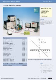
Figure 4.1: Reversible cyclic process. The shaded area of the loop is the total work done<br />
by the system in one cycle.<br />
It follows from the first law of thermodynamics that, since ∆U = 0, the work done by the<br />
system during a cycle is equal to the heat absorbed, i. e.,<br />
<br />
−∆W = ∆Q = PdV = Area enclosed.<br />
⋆ In a cyclic process, work is converted into heat and in the end of each cycle the<br />
system returns to its original state. We will introduce the heat engine which is<br />
based on the properties of a cyclic process.<br />
25
26 CHAPTER 4. ENTROPY AND SECOND LAW OF THERMODYNAMICS<br />
Let us consider the operation of a heat engine in more detail (Fig. 4.2).<br />
Part of the heat that is transferred to the system<br />
from a heat bath with temperature T1, Q1, is converted<br />
into work, W, and the rest, Q2, is delivered<br />
to a second bath with T2 < T1 (condenser). Following<br />
the first law of thermodynamics,<br />
Q1 − |Q2| = |W |.<br />
Carnot process: This a reversible cycle process<br />
bounded by two isotherms and two adiabatic lines.<br />
The Carnot process can be realized with an arbitrary<br />
working substance, but we shall consider here<br />
an ideal gas (Fig. 4.3).<br />
Figure 4.2: Heat engine.<br />
Figure 4.3: Ideal gas as a working substance for the Carnot process.<br />
In the P − V diagram the Carnot process can be represented as shown in Fig. 4.4.<br />
Figure 4.4: The Carnot process in the P − V diagram.<br />
One Carnot cycle consists of four consecutive thermodynamic processes, which are<br />
1. A → B: isothermal expansion at T = T1; the volume changes as<br />
VA → VB,<br />
while heat Q1 is absorbed from a bath and the system performs work.
4.2. SECOND LAW OF THERMODYNAMICS 27<br />
2. B → C: adiabatic expansion, during which<br />
and<br />
while δQ = 0.<br />
T1 → T2<br />
VB → VC,<br />
3. C → D: isothermal compression at T = T2; the system ejects heat Q2 to the bath<br />
(Q2 < 0 is a convention).<br />
4. D → A: adiabatic compression, during which<br />
T2 → T1,<br />
VD → VA,<br />
δQ = 0.<br />
In one cycle operation, the system receives an amount of heat Q1 from a hot reservoir,<br />
performs work, and rejects ”waste heat” Q2 to a cold reservoir.<br />
From the first law of thermodynamics we have:<br />
<br />
0 = dU = (δQ + δW) = Q + W = Q1 + Q2 + W,<br />
where −W is the work performed by the system, equal to the area enclosed in the loop<br />
(shaded area in Fig. 4.4).<br />
The efficiency of the Carnot engine is defined as<br />
η ≡<br />
performed work<br />
absorbed heat<br />
= −W<br />
Q1<br />
= Q1 + Q2<br />
Q1<br />
= Q1 − |Q2|<br />
Q1<br />
η is 100% if there is no waste heat (Q2 = 0). However, we will see that this is impossible<br />
due to the second law of thermodynamics.<br />
4.2 Second law of thermodynamics<br />
Definition by Clausius:<br />
” There is no thermodynamic transformation whose sole effect is to deliver heat<br />
from a reservoir of lower temperature to a reservoir of higher temperature.”<br />
Summary: heat does not flow upwards.<br />
Definition by Kelvin:<br />
”There is no thermodynamic transformation whose sole effect is to extract heat<br />
from a reservoir and convert it entirely to work”.<br />
Summary: a perpetuum mobile of second type does not exist.<br />
.
28 CHAPTER 4. ENTROPY AND SECOND LAW OF THERMODYNAMICS<br />
In order to prove that both definition are equivalent, we will<br />
show that the falsehood of one implies the falsehood of the<br />
other. For that purpose, we consider two heat reservoirs with<br />
temperatures T1 and T2 with T1 > T2.<br />
(1) If Kelvin’s statement were false, we could extract heat<br />
from T2 and convert it entirely to work. We could then<br />
convert the work back to heat entirely and deliver it to T1<br />
(there is no law against this) (Fig. 4.5). Thus, Clausius’<br />
statement would be negated.<br />
Figure 4.5: Q2 = W =<br />
Q1 process.<br />
(2) If Clausius’ statement were false, we could let an amount<br />
of heat Q1 flow from T2 to T1 (T2 < T1). Then, we could<br />
connect a Carnot engine between T1 and T2 such as to<br />
extract Q1 from T1 and return an amount |Q2| < Q1 back to T2. The net work<br />
output of such an engine would be |Q1| − |Q2| > 0, which would mean that an<br />
amount of heat |Q1| − |Q2| is converted into work, without any other effect. This<br />
would contradict Kelvin’s statement.<br />
From the microscopic point of view<br />
- heat transfer is an exchange of energy due to the random motion of atoms;<br />
- work’s performance requires an organized action of atoms.<br />
In these terms, heat being converted entirely into work means chaos changing spontaneously<br />
to order, which is a very improbable process.<br />
→ Usually,<br />
- one configuration corresponds to order;<br />
- many configurations correspond to chaos.
4.3. ABSOLUTE TEMPERATURE 29<br />
4.3 Absolute temperature<br />
In order to introduce the concept of absolute temperature, let us discuss the consequences<br />
of the second law of thermodynamics.<br />
i) The second law of thermodynamics implies that a Carnot engine cannot be 100%<br />
efficient since otherwise all heat absorbed from a warm reservoir would be converted<br />
into work in one cycle.<br />
ii) No engine working between two given temperatures can be more efficient than a<br />
Carnot engine.<br />
A Carnot engine is a reversible engine between two baths. The previous statement means<br />
as well that an irreversible engine cannot be more efficient than a reversible one. In order<br />
to show this, we consider two engines C and X (with X not necessarily a Carnot one)<br />
working between baths at T1 (warm) and T2 (cold). We run the Carnot engine C in<br />
reverse, as a refrigerator ¯ C, and feed the work output of X to ¯ C (Fig. 4.6).<br />
Figure 4.6: Linked engine X and Carnot refrigerator ¯ C.<br />
The total work output of such a system is<br />
Wtot = (|Q ′ 1| − |Q ′ 2|) − (|Q1| − |Q2|) .<br />
If we adjust the two engines so that |Q ′ 1 | = |Q1|, no net heat is extracted from the heat<br />
bath at T1. In this case, an amount of heat |Q2| − |Q ′ 2 | is extracted from the heat bath<br />
at T2 and converted entirely to work, with no other effect. This would violate the second<br />
law of thermodynamics unless<br />
|Q2| ≤ |Q ′ 2 |.<br />
We divide this inequality by |Q1| and, using the fact that |Q1| = |Q ′ 1 |, get<br />
and<br />
|Q2|<br />
|Q1| ≤ |Q′ 2 |<br />
|Q ′ 1|<br />
1 − |Q2|<br />
|Q1| ≥ 1 − |Q′ 2|<br />
.<br />
|<br />
|Q ′ 1
30 CHAPTER 4. ENTROPY AND SECOND LAW OF THERMODYNAMICS<br />
From this follows that the efficiencies of the engines compare as<br />
ηC ≥ ηX .<br />
Consequence: all Carnot engines have the same efficiency since X can be, as a special<br />
case, a Carnot engine.<br />
⇒ The Carnot engine is universal, i.e., it depends only on the temperatures involved<br />
and not on the working substance.<br />
Definition: absolute temperature θ of a heat reservoir (bath) is defined such that the ratio<br />
of the absolute temperatures of two reservoirs is given by<br />
θ2<br />
θ1<br />
≡ |Q2|<br />
|Q1|<br />
−Q2<br />
= 1 − η = ,<br />
where η is the efficiency of a Carnot engine operating between the two reservoirs. Since<br />
|Q2| is strictly greater than zero, |Q2| > 0, according to the second law of thermodynamics,<br />
the absolute temperature is bounded from below:<br />
θ > 0 .<br />
⋆ This means that the absolute zero θ = 0 is a limiting value that can never be reached<br />
since this would violate the second law of thermodynamics.<br />
If an ideal gas is considered as a working substance in a Carnot engine, the absolute<br />
temperature coincides with the temperature of the ideal gas defined as<br />
T = PV<br />
NkB<br />
= θ.<br />
4.4 Temperature as integrating factor<br />
The absolute temperature T can be considered as an integrating factor that converts the<br />
inexact differential δQ into an exact differential δQ/T.<br />
Let us consider the following theorem stated by Clausius:<br />
⇒ ”In an arbitrary cyclic process P, the following inequality holds:<br />
<br />
P<br />
δQ<br />
T<br />
≤ 0;<br />
where the equality holds for P reversible.“<br />
Q1
4.4. TEMPERATURE AS INTEGRATING FACTOR 31<br />
Proof. Let us divide the cycle P into n segments so that on each segment<br />
its temperature Ti (i = 1, . . .,n) is constant. We consider now a reservoir<br />
at temperature T0 > Ti(∀i) (Fig. 4.7) and introduce Carnot engines<br />
between the reservoir at T0 and Ti.<br />
Figure 4.7: Cycle P connected to the reservoir at T0 via Carnot engines.<br />
For each Carnot engine,<br />
Wi + Q (0)<br />
i + QC i<br />
For cycle P,<br />
with<br />
Q (0)<br />
i<br />
T0<br />
+ QC i<br />
Ti<br />
= 0 (first law of thermodynamics) and<br />
= 0 (definition of absolute temperature).<br />
W +<br />
n<br />
Qi = 0 (first law of thermodynamics),<br />
i=1<br />
Qi = −Q C i .<br />
Then, the total heat absorbed from the reservoir at T0 is<br />
n<br />
n Q<br />
= −T0<br />
C i<br />
= T0<br />
Q (0)<br />
T =<br />
i=1<br />
Q (0)<br />
i<br />
and the work performed by the system is<br />
<br />
n<br />
WT = − W +<br />
=<br />
n<br />
Qi +<br />
i=1<br />
i=1<br />
n<br />
i=1<br />
Wi<br />
<br />
i=1<br />
Ti<br />
<br />
Q (0)<br />
<br />
i − Qi =<br />
n<br />
i=1<br />
n<br />
i=1<br />
Q (0)<br />
i<br />
Qi<br />
Ti<br />
= Q(0)<br />
T .
32 CHAPTER 4. ENTROPY AND SECOND LAW OF THERMODYNAMICS<br />
> 0, the combined machine would convert completely the heat from reservoir at<br />
T0 into mechanical work. This would violate Kelvin’s principle and therefore<br />
If Q (0)<br />
T<br />
i.e.,<br />
For n → ∞,<br />
The theorem of Clausius is proved.<br />
T0<br />
<br />
Q (0)<br />
T<br />
n<br />
i=1<br />
P<br />
δQ<br />
T<br />
≤ 0,<br />
Qi<br />
Ti<br />
≤ 0.<br />
≤ 0 .<br />
For a reversible process, we can revert the energy, which gives us<br />
<br />
δQ<br />
≥ 0.<br />
T<br />
This implies that<br />
for a reversible process.<br />
<br />
P<br />
P<br />
δQ<br />
T<br />
= 0<br />
Corollary: for a reversible open path P, the integral<br />
<br />
dQ<br />
T<br />
depends only on the end points and not on the particular path.<br />
4.5 Entropy<br />
Since<br />
dQ<br />
T<br />
= 0 for a reversible process, δQ<br />
T<br />
P<br />
dS = δQ<br />
T<br />
Eq. (4.1) implies that there exists a state function S.<br />
is an exact differential:<br />
. (4.1)<br />
Definition: The state function S (potential), whose differential is given as<br />
is called entropy.<br />
dS = δQ<br />
T
4.5. ENTROPY 33<br />
The entropy is defined up to an additive constant. The difference between entropies of<br />
any two states A and B is<br />
B<br />
δQ<br />
S(B) − S(A) ≡<br />
T ,<br />
where the integral extends along any reversible path connecting A and B, and the result<br />
of the integration is independent of the path.<br />
What happens when the integration is along an irreversible<br />
path? Since I − R is a cycle (see Fig. 4.8), it<br />
follows from Clausius’ theorem that<br />
⇒<br />
<br />
I<br />
<br />
δQ<br />
T ≤<br />
Therefore, in general<br />
B<br />
A<br />
I−R<br />
<br />
δQ<br />
T<br />
R<br />
δQ<br />
T<br />
δQ<br />
T<br />
≤ 0 ⇒<br />
= S(B) − S(A) .<br />
≤ S(B) − S(A) ,<br />
and the equality holds for a reversible process.<br />
A<br />
Figure 4.8: I − R (irreversiblereversible)<br />
cycle.<br />
In particular, for an isolated system, which does not exchange heat with a reservoir,<br />
δQ = 0 and therefore<br />
∆S ≥ 0 .<br />
This means that the entropy of an isolated system never decreases and remains constant<br />
during a reversible transformation.<br />
Note:<br />
i) The joint system of a system and its environment is called ”universe”. Defined in this<br />
way, the ”universe” is an isolated system and, therefore, its entropy never decreases.<br />
However, the entropy of a non-isolated system may decrease at the expense of the<br />
system’s environment.<br />
ii) Since the entropy is a state function, S(B) − S(A) is independent of the path, regardless<br />
whether it is reversible or irreversible. For an irreversible path, the entropy<br />
of the environment changes, whereas for a reversible one it does not.<br />
iii) Remember that the entropy difference<br />
B<br />
S(B) − S(A) =<br />
only when the path is reversible; otherwise the difference is larger that the integral.<br />
A<br />
δQ<br />
T
34 CHAPTER 4. ENTROPY AND SECOND LAW OF THERMODYNAMICS<br />
4.6 The energy equation<br />
We note that for a reversible process in a closed system the first law of thermodynamics<br />
can be written as<br />
TdS = dU − δW = dU + PdV.<br />
Let us consider T and V as independent variables (f.i., in a gas):<br />
S = S(T, V ),<br />
U = U(T, V ) → caloric equation of state,<br />
P = P(T, V ) → thermic equation of state.<br />
Since usually the internal energy U is not directly measurable, it is more practical to<br />
consider dS = δQ/T. We will make use of one of the heat equations derived in section<br />
3.5:<br />
Dividing both sides of eq. (4.2) by T we get<br />
On the other hand,<br />
<br />
∂U ∂U<br />
δQ = dT + + P dV<br />
∂T V ∂V T <br />
∂U<br />
= CV dT + + P dV (4.2)<br />
∂V<br />
δQ<br />
T<br />
= dS = CV<br />
T<br />
dS =<br />
dT + 1<br />
T<br />
T<br />
<br />
∂U<br />
+ P dV . (4.3)<br />
∂V T<br />
<br />
∂S ∂S<br />
dT + dV . (4.4)<br />
∂T V ∂V T<br />
Comparing eq. (4.3) and (4.4), we obtain the following expressions:<br />
<br />
∂S<br />
∂T V<br />
<br />
∂S<br />
∂V<br />
T<br />
= CV<br />
T ,<br />
= 1<br />
T<br />
<br />
∂U<br />
+ P .<br />
∂V T<br />
We use the commutativity of differentiation operations,<br />
to write<br />
1<br />
T<br />
∂<br />
∂V<br />
<br />
∂U<br />
∂T V T<br />
∂<br />
∂V<br />
∂S<br />
∂T<br />
T<br />
= ∂<br />
∂T<br />
∂S<br />
∂V ,<br />
<br />
∂ CV<br />
=<br />
∂V T<br />
∂<br />
<br />
1 ∂U<br />
∂T T ∂V T<br />
= − 1<br />
T 2<br />
<br />
∂U<br />
+ P +<br />
∂V<br />
1<br />
<br />
∂<br />
T ∂T<br />
<br />
+ P ,<br />
<br />
∂U<br />
∂V T V<br />
+<br />
<br />
∂P<br />
;<br />
∂T V
4.7. USEFUL COEFFICIENTS 35<br />
we cancel identical terms:<br />
and get<br />
<br />
∂U<br />
∂V T<br />
= T<br />
∂<br />
∂V<br />
<br />
∂P<br />
∂T V<br />
<br />
∂U<br />
=<br />
∂T<br />
∂U<br />
∂T∂V<br />
− P ⇒ energy equation. (4.5)<br />
In the energy equation, the derivative of the internal energy is written in terms of measurable<br />
quantities.<br />
Examples: for an ideal gas <br />
∂U<br />
∂V T<br />
= T nR<br />
V<br />
− P = 0,<br />
which means that the internal energy of the ideal gas is not dependent on its volume:<br />
Gay-Lussac experiment:<br />
4.7 Useful coefficients<br />
U = U(T) = CV T + const.<br />
U = 3<br />
2 NkBT → gas of monoatomic molecules,<br />
U = 5<br />
2 NkBT → gas of diatomic molecules.<br />
As<br />
<br />
we<br />
<br />
saw in the last section, the energy equation relates the experimentally inaccessible<br />
∂U<br />
∂V T to the experimentally accessible <br />
∂P<br />
∂T V . We will show now that <br />
∂P<br />
can be<br />
∂T V<br />
related to other thermodynamic coefficients as well. For that purpose, we will make use<br />
of the chain rule<br />
<br />
∂x ∂y ∂z<br />
= −1 ,<br />
∂y z ∂z x ∂x y<br />
(4.6)<br />
which can be derived by considering the differential of function f(x, y, z):<br />
df = ∂f ∂f ∂f<br />
dx + dy +<br />
∂x ∂y ∂z dz,<br />
<br />
∂x<br />
∂y<br />
<br />
∂y<br />
∂z<br />
z<br />
x<br />
= − ∂f/∂y<br />
∂f/∂x ,<br />
= − ∂f/∂z<br />
∂f/∂y ,
36 CHAPTER 4. ENTROPY AND SECOND LAW OF THERMODYNAMICS<br />
Using (4.6), we get<br />
<br />
∂P<br />
∂T V<br />
where<br />
= −<br />
α = 1<br />
<br />
∂V<br />
V ∂T P<br />
kT = − 1<br />
<br />
∂V<br />
V ∂P T<br />
kS = − 1<br />
<br />
∂V<br />
V ∂P<br />
<br />
∂z<br />
= −<br />
∂x y<br />
∂f/∂x<br />
∂f/∂z .<br />
1<br />
(∂T/∂V ) P (∂V/∂P) T<br />
S<br />
= − (∂V/∂T) P<br />
(∂V/∂P) T<br />
= α<br />
kT<br />
(coefficient of thermal expansion),<br />
(isothermal compressibility),<br />
(adiabatic compressibility).<br />
We substitute in<br />
<br />
∂U<br />
δQ = TdS = CV dT + + P dV<br />
∂V T<br />
expressions (4.7) and (4.5) and get the following useful relations.<br />
, (4.7)<br />
1) The absorbed heat is expressed in terms of directly measurable coefficients as<br />
where T and V are independent variables.<br />
2) If T and P are used as independent variables, then<br />
δQ = TdS = CV dT + α<br />
TdV , (4.8)<br />
kT<br />
TdS = CPdT − αTV dP (4.9)<br />
3) If V and P are used as independent variables, dT can be rewritten in terms of dV<br />
and dP as<br />
<br />
∂T ∂T<br />
dT = dV + dP =<br />
∂V P ∂P V<br />
1 kT<br />
+ dP .<br />
αV α<br />
The corresponding TdS equation is then<br />
TdS = CP<br />
dV +<br />
αV<br />
CPkT<br />
α<br />
<br />
− αTV dP . (4.10)<br />
There is also an important connection between CP and CV (which follows from eq.<br />
(4.8) and (4.9)):<br />
CP − CV = α2<br />
TV = −T<br />
kT<br />
<br />
∂V 2<br />
∂T P<br />
∂V<br />
∂P T<br />
> 0 . (4.11)
4.8. ENTROPY AND DISORDER 37<br />
By introducing the isochore pressure coefficient<br />
it is possible to rewrite CP − CV as<br />
Indeed,<br />
β = 1<br />
P<br />
α<br />
kT<br />
⇒ CP − CV = α2<br />
β = 1<br />
P<br />
4.8 Entropy and disorder<br />
kT<br />
<br />
∂P<br />
∂T V<br />
β 2 TV kTP 2 .<br />
⇒ α = βPkT ⇒<br />
TV = β2 P 2 k 2 T<br />
kT<br />
,<br />
TV = β 2 TV kTP 2 .<br />
We want now to establish a connection between thermodynamics and statistical mechanics,<br />
which we will be learning in the second half of the course.<br />
1. We give a definition of the multiplicity of a macrostate as<br />
⎛<br />
number of microstates<br />
multiplicity of<br />
= ⎝ that correspond to the<br />
a macrostate<br />
macrostate<br />
2. The entropy can be defined in terms of the multiplicity as<br />
S ≡ k ln (multiplicity) .<br />
We shall see in statistical mechanics that this definition is equivalent to the phenomenological<br />
concept we have learnt previously in this section.<br />
3. With the above definition of entropy at hand, we can formulate the second law of<br />
thermodynamics in this way:<br />
4.<br />
”If an isolated system of many particles is allowed to change, then, with large probability,<br />
it will evolve to the macrostate of largest entropy and will remain in that<br />
macrostate.”<br />
(energy input by heating)<br />
∆Sany system ≥ ,<br />
T<br />
where T is the temperature of the reservoir.<br />
5. If two macroscopic systems are in thermal equilibrium and in thermal contact, the<br />
entropy of the composite system equals the sum of the two individual entropies.<br />
⎞<br />
⎠.
38 CHAPTER 4. ENTROPY AND SECOND LAW OF THERMODYNAMICS<br />
6. Since entropy is proportional to the ”multiplicity of a macrostate”, it can be viewed<br />
as a ”measure of disorder”:<br />
Order Disorder<br />
⇓ ⇓<br />
strong correlation absence of correlation<br />
⇓ ⇓<br />
small multiplicity large multiplicity<br />
As an illustration, let us consider a class in the school, where all kids sit always in<br />
the same place. This situation can be defined as ”ordered” since there is a strong<br />
correlation between the kids’ positions. For example, if Peter sits in the first row,<br />
you know straight away who is sitting behind and besides him: there is only one<br />
possibility (multiplicity is very low).<br />
Looking now at a class in the kindergarten, we will find that the children there are<br />
all mixed, sitting and moving all the time. Now, if Peter sits in the first row, you<br />
have no idea where the other kids are sitting. There are no correlations between the<br />
kids’ positions and there are many options to have the children in the class. Such a<br />
”system” of kids is in a ”disordered state”, with very high multiplicity. The entropy<br />
of the kindergarten class is high!<br />
4.9 Third law of thermodynamics (Nernst law)<br />
While with the second law of thermodynamics we can only define the entropy (up to a<br />
constant), the third law of thermodynamics tells us how S(T) behaves at T → 0. Namely,<br />
it states that the entropy of a thermodynamic system at T = 0 is a universal constant,<br />
that we take to be 0:<br />
lim S(T) = 0.<br />
T →0<br />
S(T → 0) is independent from the values that the rest of variables take.<br />
Consequences:<br />
1) The heat capacities of all substances disappear at T = 0:<br />
lim<br />
T →0 CV<br />
<br />
∂S<br />
= lim T = 0,<br />
T →0 ∂T V<br />
lim<br />
T →0 CP<br />
<br />
∂S<br />
= lim T = 0.<br />
T →0 ∂T P<br />
Note that an ideal gas provides a contradiction to the previous statement since in<br />
that case CV = const and CP = const:<br />
CV = 3<br />
2 NkB,<br />
CP = CV + NkB = 5<br />
2 NkB,<br />
CP − CV = NkB = 0. (4.12)
4.9. THIRD LAW OF THERMODYNAMICS (NERNST LAW) 39<br />
2)<br />
But, for T → 0 the ideal gas is not anymore a realistic system because a real gas<br />
undergoes at low temperatures a phase transition - condensation.<br />
lim β = lim<br />
T →0 T →0<br />
3) The absolute T = 0 (zero point) is unattainable.<br />
1<br />
V<br />
<br />
∂V<br />
= 0<br />
∂T<br />
In order to show the validity of the last statement, let us analyze what happens when we<br />
are trying to reach low temperatures by subsequently performing adiabatic and isothermal<br />
transformations. If a gas is used as a working substance (Linde method), such a sequence<br />
of transformations looks in the P − V diagram as shown in Fig. 4.9.<br />
Figure 4.9: Linde method: sequence of adiabatic and isothermal transformations in a gas.<br />
Let us consider now the processes involved.<br />
A → B: isothermic compression.<br />
Work is performed on the gas and an amount of heat Q1 < 0 is given to the reservoir<br />
in a reversible process. As a result, ∆S = Q1<br />
T diminishes.<br />
B → C: adiabatic expansion.<br />
The gas performs work. Since δQ = 0, the entropy remains constant and the<br />
temperature diminishes.
40 CHAPTER 4. ENTROPY AND SECOND LAW OF THERMODYNAMICS<br />
In principle, by repeating this process many times, one could reach the T = 0 point.<br />
But, according to the third law of thermodynamics, all entropy curves must end at 0 for<br />
T → 0, which means that only through an infinite number of steps is it possible to reach<br />
T = 0.