polar stereographic projection on the calculation of

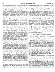
658 MONTHLY WEATHER REVIEW Vol. 96, No. 9
THE EFFECT OF POLAR STEREOGRAPHIC PROJECTION ON THE CALCULATION OF
THE CURVATURE OF HORIZONTAL CURVES*
K. KRISHNA
Poona, India
ABSTRACT
It is shown that, in any secant <strong>polar</strong> <strong>stereographic</strong> <strong>projection</strong>, a small circle on a sphere projects into a circle.
This property provides a simple relationship between KH, the horizontal component of curvature of a horizonal
curve and Kb, the curvature of its <strong>projection</strong> on a secant <strong>polar</strong> <strong>stereographic</strong> map. KH can be computed by sub-
tracting from the map factor times Kh the earth’s curvature multiplied by a correction factor that depends only
on the latitude of the place and inclination of the curve to the latitude circle. This factor vanishes if tho curve is
along a meridian but takes an extreme value if it is along a latitude. For a given orientation of the curve, the value
of this factor incrcases gradually as the location of the curve moves from the Pole to the Equator and more rapidly
after it crosscs the Equator. It is less than 1 in the Northern Hemisphere but can exceed unity in the Southern
Hemisphere.
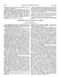
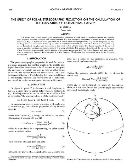
1. INTRODUCTION
The <strong>polar</strong> <strong>stereographic</strong> <strong>projection</strong> is used for several
purposes, especially for weather charts in the middle and
higher latitudes. Sometimes it is of interest to compute
the curvature of certain contours as well as other types
of curves like isobars from the curvature of their <strong>projection</strong>s
on this chart. The following derivation establishes
a relationship between the curvatures of a horizontal
curve and its <strong>projection</strong> on a <strong>polar</strong> <strong>stereographic</strong> chart.
2. DERIVATION
rn figure 1, Point p (colatitude J. and longitude
lies on a circle with its center below point C (colatitude
$o). The longitude of C can be taken as 0’ without loss
of generality. The angular radius, b, of the circle is given by
cos b=cos $o cos $+sin $o sin $ cos A. (1)
In circum<strong>polar</strong> <strong>stereographic</strong> <strong>projection</strong> with scale true
at colatitude $1, the radius of <strong>projection</strong> of any latitude
circle is
r=c tan $12 (2)
where c=a(l+cos $J, a being the radius of the earth.
Eliminating $I between (1) and (2)
2-2rd COS A-C’
which is a quadratic in r representing, in <strong>polar</strong> coordi-
nates, a circle of radius,
rL=c
COS $O-COS b-
cos $o+cos b-’
sin b
(cos tj0+ cos b)
with center at distance from the Pole,
d=c
sin $o
(cos $o+cos b)’
Equation (3) proves that a small circle on a sphere pro-
(3)
(4)
*These results were presented at a meeting of the Poona Branch of the Indian Meteore
logical Society in 1960 in the course of a talk on “Conformal Map Projections Used in
Meteorology .”
(5)
jects into a circle on the <strong>projection</strong> in question. The
curvature Of the latter is
COS $OS COS b
K&=
G sin b
Taking the spherical triangle NCP (fig. I), it can be
shown that
~ ~ (KL- = m
a(l+cos sin
(6)
cos $1) /3 )
where KH is the horizontal curvature of the original
circle, m is the scale factor, and /3 is the angle between the
curve and the latitude
N
I
S
FIGURE 1.-The coordinates of a point on a small circle on a sphere.

September 1968 K. Krishna 659
The values of KH and m are
Equation (6) provides a relationship between KH and
K‘H in terms of m, 0, +, &. In the case of a tangent <strong>polar</strong>
<strong>stereographic</strong> <strong>projection</strong> (+1=0), this reduces to
as given by Haltiner and Martin [l].
Equation (6) provides a value for the error E, the
difference between the curvature of the curve and curva-
ture of its <strong>projection</strong> adjusted for scale.
t 1 *
E=KH-mKH=-- tan - cos /3.
a 2
E is, however, independent of the location of the
standard parallel. It vanishes at points V and V’ (see
fig. 1) where the curve touches the meridian. Its magni-
tude has maximum and minimum values at points X and
M respectively, i.e., when the curve touches a latitude
circle. The magnitude of the extreme value of the error
is tan +/2 times the curvature of the earth. Thus, in the
Northern Hemisphere (for <strong>projection</strong> from the South
Pole) where + is less than go”, the error is always less
than the curvature of the earth and it increases as the
latitude decreases. As the location moves into the South-
ern Hemisphere, it can exceed unity.
3. DISPLACEMENT OF THE CENTER OF CURVATURE
Whereas a circle projects into a circle, its center does not
project into the center of its <strong>projection</strong>. The center of
the <strong>projection</strong> of the circle lies farther away from the
Pole than the <strong>projection</strong> of the center of the circle.
Figure 2 represents a cross section of the sphere shown
in figure 1 along the meridional plane passing through C.
The diameter MX of the small circle projects into M’X’
and the center C into C’. P’ is the midpoint of M’X’.
It is evident that P’ and C’ are not one and the same,
since MC and CX will not project into equal lengths. If
the angular shift of the center of the circle (viz CP) is
a degrees from the Pole, from (2) and (5)
sin +o
tan *0+a -- -
2 (COS +~+COS b)
Expanding the above equation in terms of tangents of
half angles of a, b, and +o and solving for tan a12
If a and b are expressed in degrees we have, for small
values of b, the approximate relationship,
(8)
(9)
[Received December 21, 1967; revised March IS, 19681
N
S
FIGURE 2.-Cross section of a sphere, a small circle and
its <strong>projection</strong>.
If the center of the circle lies on the Equator the appar-
ent shift of the center of the <strong>projection</strong> of a circle is
approximately 15’ and 1’ for circles of radius 5’ and 10’
respectively. The corresponding values for circles with
centers at 30’N. lat. are 9’ and 35’ respectively.
Since the center of the projected circle is not the same
as the <strong>projection</strong> of the center of the small circle, con-
centric small circles other than latitude circles will not
project into concentric circles. The centers of the pro-
jection of these concentric circles will be different and will
lie on the same meridian; the center of a circle with larger
radius will be displaced farther away from Pole.
The complications introduced by the distortions due
to the <strong>projection</strong> can be avoided if the diameter of the
circle of curvature is taken as the difference in the lati-
tudes of the points M and X where the meridian through
the center intersects the circle of curvature and K H is
calculated from its definition (see equation (6)).
ACKNOWLEDGMENT
I am grateful to Dr. Bh. V. Ramana Murty for his meticulous
examination of the manuscript and for the suggestions which led
to considerable improvement in the presentation of the paper.
REFERENCE
1. G. J. Haltiner and F. L. Martin, Dynamical and Physical
Meteorology, McGraw-Hill Book Company, Inc., New York,
1957, 470 pp. (see p. 175).

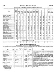
660
Mesoscale cloud patterns are strongly influenced by the
terrain features of an area. A frequently observed example
is the formation of wave clouds in the area of gravity
waves to the lee of mountains. These clouds occur when:
the wind direction .is perpendicular to the mountains
through a deep layer, the mountain top wind is a minimum
of 20 kt., and the atmosphere is stable for vertical dis-
placements of air. Satellite photographs show that the
unique parallel arrangement of small wave clouds is
common to all major mountain chains throughout the
world. In the Uhited States, lee waves are frequently
observed, as in this case, along the northwestern ranges.
On June 21, 1968, the 1200 GMT analysis showed a weak
surface High centered in Wyoming with a low pressure
area off the Washington coast. The 500- and 300-mb.
analysis showed strong zonal flow across the northwestern
United States. At this time, the 200-mb. jet stream was
analyzed to cross the coast near Seattle and follow a path,
due east, along 48'N. through Idaho and Montana and
then northeastward into Canada.
Upper air solindings for 1200 GMT at Lander, Wyo.
(LND), and Great Falls, Mont. (GTF), accompany the
1435 GMT ESSA-2 photograph in figure 1. At this time,
low clouds are present near LND and middle and high
clouds at GTF. Little directional wind shear is indicated
at both these stations.
The ESSA-5 picture (fig. 2), taken at 2309 GMT, shows
that late morning and early afternoon convection in this
area has resulted in a large area of wave clouds through
Idaho, Montana, and Wyoming. The 0000 GMT soundings
at both stations show the lapse rate to be dry adiabatic
up to the base of the inversion. At GTF the winds aloft
have increased due to a shift in the jet stream; now
entering the coast at 49'N., it continues eastward to
115OW. and gradually turns southeastward passing
through the extreme southwest corner of North Dakota.
The brightest group of wave clouds (Q) is found near
the 6,000- to 9,000-ft. Cabinet Mountains and the Bitter
Root Range. The clouds become more widely spaced to
the east in the vicinity of the Rocky Mountains of
Montana. The upper air data at GTF indicates that the
wind at the mountain top level is greater than 26 kt. from
the west-southwest.
~
MONTHLY WEATHER REVIEW
PICTURE OF THE MONTH
FRANCES C. PARMENTER
National Environmental Satellite Center, ESSA, Washington, D.C.
!
i
\
Vol. 96, No. 9
TEMP 8 DEWPDINT
WIND SPEED
TEMP. 8 DEWPDINT WIND SPEED
('t) (Knot.) (.C.) (Knot.)
LND 576 12DDGMT June 21. 1960 GTF 775 1200GMT June 21. 1960
FIGURE 1.-ESSA 2, APT, Orbit 10705, 1436 GMT and 1200 GMT,
The wave cloud pattern to the south (R) is in the umer air soundings for Lander, Wvo. (LND). and Great Falls,
I " . .,
vicinity of the higher Rocky Mountains in Wyoming and Mint. (GTF), JU& 21, 1968.
i '

September 1968 Frances C. Parmenter 661
southern Montana. These clouds lie to the north of
Yellowstone Park, and along the north-south Absaroka
and Wind River Ranges, and farther east along the Big
Horn Mountains. The wind at the top of the 12,000- and
14,000-ft. mountains, indicated by LND, is 40 kt. from
the west.
Another area of wave clouds (S) can be seen along the
eastern edge of the frontal cloudiness approaching Wash-
ington and Oregon, in the vicinity of Mt. Adams and
Mt. Hood.
The presence of wave clouds in satellite photographs
provides the aviation forecaster with visual information
20 I I 'J0' I ',L
TEMP. B DEWPOINT WIND SPEED
I'C) (Knots1
LND 576 OOOOGMT June 22,1968
I 1 1 1 11 I 1 I 1 IIAII 1211 i - dli; I 1;; 1 1 ~ ~ ~
-60 -40 -20
TEMP B DEWPOINT WIND SPEED
(.C I (Knolrl
GTF 771 OOOOGMT June 22.1960
FIGURE 2.-ESSA 5, Orbit 5431, 2309 GMT, June 21, 1968, and 0000
GMT, upper air soundings for Lander, Wyo. (LND), and Great
Falls, Mont. (GTF), June 22, 1968.
about the mesoscale wind patterns and general atmos-
pheric structure in the vicinity of mountainous areas.
Although the distribution of turbulence associated with
lee waves is still under investigation, some preliminary
results indicate that the turbuleiit layer is confined to the
area within and below these clouds. Soaring and glideplane
pilots were among the first to investigate wave clouds,
and by flying these clouds, these pilots have established
new height and distance records. Using the same tech-
nique, light aircraft pilots have found that they can
conserve fuel by "riding" the wave clouds.