Abstract - Project Links - Rensselaer Polytechnic Institute
Abstract - Project Links - Rensselaer Polytechnic Institute
Abstract - Project Links - Rensselaer Polytechnic Institute

Create successful ePaper yourself
Turn your PDF publications into a flip-book with our unique Google optimized e-Paper software.
UMAP<br />
The<br />
Journal<br />
Publisher<br />
COMAP, Inc. Vol. 29, No. 3<br />
Executive Publisher<br />
Solomon A. Garfunkel<br />
ILAP Editor<br />
Chris Arney<br />
Division Chief,<br />
Mathematical Sciences<br />
Program Manager,<br />
Cooperative Systems<br />
Army Research Office<br />
P.O. Box 12211<br />
Research Triangle Park,<br />
NC 27709-2211<br />
david.arney1@arl.army.mil<br />
On Jargon Editor<br />
Yves Nievergelt<br />
Dept. of Mathematics<br />
Eastern Washington Univ.<br />
Cheney, WA 99004<br />
ynievergelt@ewu.edu<br />
Reviews Editor<br />
James M. Cargal<br />
Mathematics Dept.<br />
Troy University—<br />
Montgomery Campus<br />
231 Montgomery St.<br />
Montgomery, AL 36104<br />
jmcargal@sprintmail.com<br />
Chief Operating Officer<br />
Laurie W. Aragón<br />
Production Manager<br />
George W. Ward<br />
Production Editor<br />
Joyce Barnes<br />
Distribution<br />
John Tomicek<br />
Graphic Designer<br />
Daiva Chauhan<br />
Editor<br />
Paul J. Campbell<br />
Beloit College<br />
700 College St.<br />
Beloit, WI 53511–5595<br />
campbell@beloit.edu<br />
Associate Editors<br />
Don Adolphson<br />
Chris Arney<br />
Aaron Archer<br />
Ron Barnes<br />
Arthur Benjamin<br />
Robert Bosch<br />
James M. Cargal<br />
Murray K. Clayton<br />
Lisette De Pillis<br />
James P. Fink<br />
Solomon A. Garfunkel<br />
William B. Gearhart<br />
William C. Giauque<br />
Richard Haberman<br />
Jon Jacobsen<br />
Walter Meyer<br />
Yves Nievergelt<br />
Michael O’Leary<br />
Catherine A. Roberts<br />
John S. Robertson<br />
Philip D. Straffin<br />
J.T. Sutcliffe<br />
Brigham Young Univ.<br />
Army Research Office<br />
AT&T Shannon Res. Lab.<br />
U. of Houston—Downtn<br />
Harvey Mudd College<br />
Oberlin College<br />
Troy U.— Montgomery<br />
U. of Wisc.—Madison<br />
Harvey Mudd College<br />
Gettysburg College<br />
COMAP, Inc.<br />
Calif. State U., Fullerton<br />
Brigham Young Univ.<br />
Southern Methodist U.<br />
Harvey Mudd College<br />
Adelphi University<br />
Eastern Washington U.<br />
Towson University<br />
College of the Holy Cross<br />
Georgia Military College<br />
Beloit College<br />
St. Mark’s School, Dallas
Subscription Rates for 2008 Calendar Year: Volume 29<br />
Institutional Web Membership (Web Only)<br />
Institutional Web Memberships does not provide print materials. Web memberships<br />
allow members to search our online catalog, download COMAP print materials, and reproduce<br />
for classroom use.<br />
(Domestic) #2830 $449 (Outside U.S.) #2830 $449<br />
Institutional Membership (Print Only)<br />
Institutional Memberships receive print copies of The UMAP Journal quarterly, our<br />
annual CD collection UMAP Modules, Tools for Teaching, and our organizational<br />
newsletter Consortium.<br />
(Domestic) #2840 $289 (Outside U.S.) #2841 $319<br />
Institutional Plus Membership (Print Plus Web)<br />
Institutional Plus Memberships receive print copies of the quarterly issues of The UMAP<br />
Journal, our annual collection UMAP Modules, Tools for Teaching, our organizational<br />
newsletter Consortium, and on-line membership that allows members to search our online<br />
catalog, download COMAP print materials, and reproduce for classroom use.<br />
(Domestic) #2870 $569 (Outside U.S.) #2871 $599<br />
For individual membership options visit<br />
www.comap.com for more information<br />
To order, send a check or money order to COMAP, or call toll-free<br />
1-800-77-COMAP (1-800-772-6627).<br />
The UMAP Journal is published quarterly by the Consortium for Mathematics and Its<br />
Applications (COMAP), Inc., Suite 3B, 175 Middlesex Tpke., Bedford, MA, 01730, in cooperation<br />
with the American Mathematical Association of Two-Year Colleges<br />
(AMATYC), the Mathematical Association of America (MAA), the National Council of<br />
Teachers of Mathematics (NCTM), the American Statistical Association (ASA), the<br />
Society for Industrial and Applied Mathematics (SIAM), and The <strong>Institute</strong> for Operations<br />
Research and the Management Sciences (INFORMS). The Journal acquaints readers<br />
with a wide variety of professional applications of the mathematical sciences and<br />
provides a forum for the discussion of new directions in mathematical education<br />
(ISSN 0197-3622).<br />
Periodical rate postage paid at Boston, MA and at additional mailing offices.<br />
Send address changes to: info@comap.com<br />
COMAP, Inc., Suite 3B, 175 Middlesex Tpke., Bedford, MA, 01730<br />
© Copyright 2007 by COMAP, Inc. All rights reserved.
Vol. 29, No. 3 2008<br />
Table of Contents<br />
Publisher’s Editorial<br />
Change<br />
Solomon A. Garfunkel .......................................... 185<br />
About This Issue....................................................... 186<br />
Special Section on the MCM<br />
Results of the 2008 Mathematical Contest<br />
in Modeling<br />
Frank Giordano .................................................... 187<br />
<strong>Abstract</strong>s of the Outstanding Papers<br />
and the Fusaro Papers ......................................... 223<br />
The Impending Effects of North Polar Ice Cap Melt<br />
Benjamin Coate, Nelson Gross,<br />
and Megan Longo................................................. 237<br />
A Convenient Truth: Forecasting Sea Level Rise<br />
Jason Chen, Brian Choi, and ................................. 249<br />
Fighting the Waves: The Effect of North Polar<br />
Ice Cap Melt on Florida<br />
Amy M. Evans and Tracy L. Stepien....................... 267<br />
Erosion in Florida: A Shore Thing<br />
Matt Thies, Bob Liu, and Zachary W. Ulissi ............ 285<br />
Judge’s Commentary: The Polar Melt Problem Papers<br />
John L. Scharf ...................................................... 301<br />
A Difficulty Metric and Puzzle Generator for Sudoku<br />
Christopher Chang, Zhou Fan, and Yi Sun ............. 305<br />
Taking the Mystery Out of Sudoku Difficulty:<br />
An Oracular Model<br />
Sarah Fletcher, Frederick Johnson, and<br />
David R. Morrison ............................................... 327<br />
Difficulty-Driven Sudoku Puzzle Generation<br />
Martin Hunt, Christopher Pong, and<br />
George Tucker ..................................................... 343<br />
Ease and Toil: Analyzing Sudoku<br />
Seth B. Chadwick , Rachel M. Krieg, and<br />
Christopher E. Granade ........................................ 363<br />
Cracking the Sudoku: A Deterministic Approach<br />
David Martin, Erica Cross, and Matt Alexander ..... 381
Publisher’s Editorial<br />
Change<br />
Solomon A. Garfunkel<br />
Executive Director<br />
COMAP, Inc.<br />
175 Middlesex Turnpike, Suite 3B<br />
Bedford , MA 01730–1459<br />
s.garfunkel@mail.comap.com<br />
Publisher’s Editorial 185<br />
This is the season of change—for good and bad. As I write this editorial,<br />
the election is a little less than a month away. The financial markets<br />
are imploding and the country appears more than ready to head in a new<br />
direction, even if it is unsure where that direction will take us. By the time<br />
you read this, many things will be clear. We will have a new administration,<br />
perhaps a very new administration. And we will likely be living<br />
individually and collectively on less—perhaps a lot less.<br />
No matter. Some things still need to be done. I won’t speak in this forum<br />
about health care or infrastructure or other changes in foreign and domestic<br />
policy—but I will speak of mathematics education. As small as our<br />
issues may seem at times of national and international stress, education—<br />
especially technical education—can always provide a way out and up. We<br />
cry out for mathematical and quantitative literacy, not because we are lobbyists<br />
or a special interest group trying to raise teacher salaries. We cry out<br />
for literacy because knowledge is the only way to prevent the abuses whose<br />
consequences we now endure.<br />
How many times in these last few months have we heard about people<br />
who didn’t understand the terms of their mortgages; of managers and<br />
bankers who didn’t understand their degree of risk; of policy makers who<br />
didn’t understand how the dominos could fall? Yes, derivatives are confusing.<br />
And yes, derivatives of derivatives are more confusing. But isn’t this<br />
just a perfect example of why we talk about teaching mathematical modeling<br />
as a life skill? Mathematics education is not a zero-sum game. We<br />
don’t want our students to learn more mathematics than other countries’<br />
students. That is just a foolish argument used to raise money, that is, the<br />
fear that another country will out perform us or another state will take our<br />
The UMAP Journal 29 (3) (2008) 185–186. c○Copyright 2008 by COMAP, Inc. All rights reserved.<br />
Permission to make digital or hard copies of part or all of this work for personal or classroom use<br />
is granted without fee provided that copies are not made or distributed for profit or commercial<br />
advantage and that copies bear this notice. <strong>Abstract</strong>ing with credit is permitted, but copyrights<br />
for components of this work owned by others than COMAP must be honored. To copy otherwise,<br />
to republish, to post on servers, or to redistribute to lists requires prior permission from COMAP.
186 The UMAP Journal 29.3 (2008)<br />
high tech jobs.<br />
The problem is much, much bigger. There simply are not enough<br />
mathematically-trained people in the world to run the world. The proof of<br />
that statement is all around us. And it is as much in our interest that the<br />
world’s people become more quantitatively literate as it is that the citizens<br />
of our city, our state, and our country do. In theory, now there is less money<br />
to fund changes in mathematics education. But we must. We must see the<br />
issues and problems, as global issues and problems and work together to<br />
solve them.<br />
The good news is that the energy and commitment to do the job are<br />
here. At the recent conference on the Future of Mathematics Education,<br />
co-sponsored by Math is More, I met with mathematics and mathematics<br />
education researchers, with college and high school faculty, with state<br />
and local administrators, with policy-makers, and with employers. We no<br />
longer talked about why; we talked about how. The need and desire for<br />
real change was palpable. And the energy was both exciting and challenging.<br />
People kept asking, “What can I do?”—as a classroom teacher, as a<br />
supervisor of mathematics, as a staff developer, as a curriculum developer,<br />
as a policy maker.<br />
So while the times and problems are difficult, the will for positive change<br />
is here. Now is the time for all of us to gather together to make that change<br />
a reality.<br />
About This Issue<br />
Paul J. Campbell<br />
Editor<br />
This issue runs longer than a regular 92-page issue, to more than 200<br />
pages. However, not all of the articles appear in the paper version. Some<br />
appear only on the Tools for Teaching 2008 CD-ROM (and at http://www.<br />
comap.com for COMAP members), which will reach members and subscribers<br />
later and will also contain the entire 2008 year of Journal issues.<br />
All articles listed in the table of contents are regarded as published in<br />
the Journal. The abstract of each appears in the paper version. Pagination<br />
of the issue runs continuously, including in sequence articles that do not<br />
appear in the paper version. So if, say, p. 250 in the paper version is followed<br />
by p. 303, your copy is not necessarily defective! The articles on the intervening<br />
pages are on the CD-ROM.<br />
We hope that you find this arrangement agreeable. It means that we do<br />
not have to procrusteanize the content to fit a fixed number of paper pages.<br />
We might otherwise be forced to select only two or three Outstanding MCM<br />
papers to publish. Instead, we continue to bring you the full content.
Modeling Forum<br />
Results of the 2008 MCM 187<br />
Results of the 2008<br />
Mathematical Contest in Modeling<br />
Frank Giordano, MCM Director<br />
Naval Postgraduate School<br />
1 University Circle<br />
Monterey, CA 93943-5000<br />
frgiorda@nps.navy.mil<br />
Introduction<br />
A total of 1,159 teams of undergraduates, from 338 institutions and 566<br />
departments in 14 countries, spent the first weekend in February working on<br />
applied mathematics problems in the 24th Mathematical Contest in Modeling.<br />
The 2008 Mathematical Contest in Modeling (MCM) began at 8:00 P.M. EST<br />
on Thursday, February 14 and ended at 8:00 P.M. EST on Monday, February 18.<br />
During that time, teams of up to three undergraduates were to research and<br />
submit an optimal solution for one of two open-ended modeling problems.<br />
Students registered, obtained contest materials, downloaded the problems at<br />
the appropriate time, and entered completion data through COMAP’s MCM<br />
Website. After a weekend of hard work, solution papers were sent to COMAP<br />
on Monday. The top papers appear in this issue of The UMAP Journal.<br />
Results and winning papers from the first 23 contests were published in<br />
special issues of Mathematical Modeling (1985–1987) and The UMAP Journal<br />
(1985–2007). The 1994 volume of Tools for Teaching, commemorating the tenth<br />
anniversary of the contest, contains the 20 problems used in the first 10 years<br />
of the contest and a winning paper for each year. That volume and the special<br />
MCM issues of the Journal for the last few years are available from COMAP. The<br />
1994 volume is also available on COMAP’s special Modeling Resource CD-ROM.<br />
Also available is The MCM at 21 CD-ROM, which contains the 20 problems<br />
from the second 10 years of the contest, a winning paper from each year, and<br />
advice from advisors of Outstanding teams. These CD-ROMs can be ordered<br />
from COMAP at http://www.comap.com/product/cdrom/index.html .<br />
The UMAP Journal 29 (3) (2008) 187–222. c○Copyright 2008 by COMAP, Inc. All rights reserved.<br />
Permission to make digital or hard copies of part or all of this work for personal or classroom use<br />
is granted without fee provided that copies are not made or distributed for profit or commercial<br />
advantage and that copies bear this notice. <strong>Abstract</strong>ing with credit is permitted, but copyrights<br />
for components of this work owned by others than COMAP must be honored. To copy otherwise,<br />
to republish, to post on servers, or to redistribute to lists requires prior permission from COMAP.
188 The UMAP Journal 29.3 (2008)<br />
This year’s Problem A asked teams to consider the effects on land from<br />
the melting of the North Polar ice cap due to the predicted increase in global<br />
temperatures. Specifically, teams were asked to model the effects on the coast of<br />
Florida due to the melting every 10 years for the next 50 years, with particular<br />
attention to large metropolitan areas. Additionally, they were asked to propose<br />
appropriate responses to deal with the melting.<br />
Problem B asked teams to develop an algorithm to construct Sudoku puzzles<br />
of varying difficulty. The problem required teams to develop metrics to<br />
define a difficulty level. Further, the team’s algorithm and metrics were to be<br />
extensible to a varying number of difficulty levels, and they should illustrate<br />
their algorithm with at least four difficulty levels. The team’s solution had to<br />
analyze the complexity of their algorithm.<br />
The 9 Outstanding solution papers are published in this issue of The UMAP<br />
Journal, along with relevant commentaries.<br />
In addition to the MCM, COMAP also sponsors the Interdisciplinary Contest<br />
in Modeling (ICM) and the High School Mathematical Contest in Modeling<br />
(HiMCM). The ICM runs concurrently with MCM and offers a modeling problem<br />
involving concepts in operations research, information science, and interdisciplinary<br />
issues in security and safety. The 2009 problem will have an environmental<br />
science theme. Results of this year’s ICM are on the COMAP Website<br />
at http://www.comap.com/undergraduate/contests; results and Outstanding<br />
papers appeared in Vol. 29 (2008), No. 2. The HiMCM offers high<br />
school students a modeling opportunity similar to the MCM. Further details<br />
about the HiMCM are at http://www.comap.com/highschool/contests.<br />
Problem A: Take a Bath<br />
Consider the effects on land from the melting of the North Polar ice cap<br />
due to the predicted increase in global temperatures. Specifically, model the<br />
effects on the coast of Florida every 10 years for the next 50 years due to the<br />
melting, with particular attention given to large metropolitan areas. Propose<br />
appropriate responses to deal with this. A careful discussion of the data used<br />
is an important part of the answer.<br />
Problem B: Creating Sudoku Puzzles<br />
Develop an algorithm to construct Sudoku puzzles of varying difficulty.<br />
Develop metrics to define a difficulty level. The algorithm and metrics should<br />
be extensible to a varying number of difficulty levels. You should illustrate the<br />
algorithm with at least 4 difficulty levels. Your algorithm should guarantee a<br />
unique solution. Analyze the complexity of your algorithm. Your objective<br />
should be to minimize the complexity of the algorithm and meet the above<br />
requirements.
The Results<br />
Results of the 2008 MCM 189<br />
The solution papers were coded at COMAP headquarters so that names<br />
and affiliations of the authors would be unknown to the judges. Each paper<br />
was then read preliminarily by two “triage” judges at either Appalachian State<br />
University (Polar Melt Problem) or at the National Security Agency (Sudoku<br />
Problem). At the triage stage, the summary and overall organization are the<br />
basis for judging a paper. If the judges’ scores diverged for a paper, the judges<br />
conferred; if they still did not agree, a third judge evaluated the paper.<br />
AdditionalRegionalJudgingsites were created at the U.S. MilitaryAcademy<br />
and at the Naval Postgraduate School to support the growing number of contest<br />
submissions.<br />
Final judging took place at the Naval Postgraduate School, Monterey, CA.<br />
The judges classified the papers as follows:<br />
Honorable Successful<br />
Outstanding Meritorious Mention Participation Total<br />
Polar Melt Problem 4 64 182 315 565<br />
Sudoku Problem 5 95 296 198 594<br />
9 159 378 513 1159<br />
The 9 papers that the judges designated as Outstanding appear in this special<br />
issue of The UMAP Journal, together with commentaries. We list those<br />
teams and the Meritorious teams (and advisors) below; the list of all participating<br />
schools, advisors, and results is in the Appendix.<br />
Outstanding Teams<br />
Institution and Advisor Team Members<br />
Polar Melt Papers<br />
“The Impending Effects of North Polar<br />
Ice Cap Melt”<br />
College of Idaho<br />
Caldwell, ID<br />
Michael P. Hitchman<br />
“A Convenient Truth: Forecasting<br />
Sea Level Rise”<br />
Duke University<br />
Durham, NC<br />
Scott McKinley<br />
Benjamin Coate<br />
Nelson Gross<br />
Megan Longo<br />
Jason Chen<br />
Brian Choi<br />
Joonhahn Cho
190 The UMAP Journal 29.3 (2008)<br />
“Fighting the Waves: The Effect of North<br />
Polar Ice Cap Melt on Florida”<br />
University at Buffalo<br />
Buffalo, NY<br />
John Ringland<br />
“Erosion in Florida: A Shore Thing”<br />
University of Delaware<br />
Newark, DE<br />
Louis Frank Rossi<br />
“A Difficulty Metric and<br />
Puzzle Generator for Sudoku”<br />
Harvard University<br />
Cambridge, MA<br />
Clifford H. Taubes<br />
“Taking the Mystery out of Sudoku<br />
Difficulty: An Oracular Model”<br />
Harvey Mudd College<br />
Claremont, CA<br />
Jon Jacobsen<br />
“Difficulty-Driven Sudoku Puzzle<br />
Generation”<br />
Harvey Mudd College<br />
Claremont, CA<br />
Zach Dodds<br />
“Ease and Toil: Analyzing Sudoku”<br />
University of Alaska Fairbanks<br />
Fairbanks, AK<br />
Orion S. Lawlor<br />
“Cracking the Sudoku:<br />
A Deterministic Approach”<br />
Youngstown State University<br />
Youngstown, OH<br />
George T. Yates<br />
Sudoku Papers<br />
Amy M. Evans<br />
Tracy L. Stepien<br />
Matt Thies<br />
Bob Liu<br />
Zachary W. Ulissi<br />
Christopher Chang<br />
Zhou Fan<br />
Yi Sun<br />
Sarah Fletcher<br />
Frederick Johnson<br />
David R. Morrison<br />
Martin Hunt<br />
Christopher Pong<br />
George Tucker<br />
Seth B. Chadwick<br />
Rachel M. Krieg<br />
Christopher E. Granade<br />
David Martin<br />
Erica Cross<br />
Matt Alexander
Meritorious Teams<br />
Results of the 2008 MCM 191<br />
Polar Melt Problem (65 teams)<br />
Ann Arbor Huron High School, Mathematics, Ann Arbor, MI (Peter A. Collins)<br />
Beihang University, Beijing, China (HongYing Liu)<br />
Beijing Normal University, Beijing, Beijing, China (Li Cui)<br />
Beijing Normal University, Beijing, (Laifu Liu)<br />
Beijing University of Posts & Telecommunications, Electronic Engineering, Beijing,<br />
China (Zuguo He)<br />
Beijing University of Posts & Telecommunications, Applied Mathematics, Beijing,<br />
China (Hongxiang Sun)<br />
Central South University, Mechanical Design and Manufacturing Automation,<br />
Changsha, Hunan, China (Xinge Liu)<br />
Central University of Finance and Economics, Applied Mathematics, Beijing, China<br />
(Donghong Li)<br />
China University of Mining and Technology, Beijing, China (Lei Zhang) (two teams)<br />
China University of Petroleum (Beijing), Beijing, China (Ling Zhao)<br />
China University of Petroleum (East China), Qingdao, Shandong, China<br />
(Ziting Wang)<br />
Chongqing University, Applied Chemistry, Chongqing, China (Zhiliang Li)<br />
College of Charleston, Charleston, SC (Amy Langville)<br />
Concordia College–New York, Bronxville, NY (Karen Bucher)<br />
Dalian University of Technology, Software, Dalian, Liaoning, China (Zhe Li)<br />
Donghua University, Shanghai China (Liangjian Hu)<br />
Duke University, Durham, NC ( Mark Huber)<br />
East China University of Science and Technology, Physics, Shanghai, China<br />
(Lu ,hong)<br />
Gannon University, Mathematics, Erie, PA (Jennifer A. Gorman)<br />
Hangzhou Dianzi Unniversity, Information and Mathematics Science, Hangzhou,<br />
Zhejiang, China (Wei Li)<br />
Harbin <strong>Institute</strong> of Technology Shiyan School, Mathematics, Harbin, Heilongjiang,<br />
China (Yunfei Zhang)<br />
Hiram College, Hiram, OH (Brad S. Gubser)<br />
McGill University, Mathematics and Statistics, Montreal, Quebec, Canada<br />
(Nilima Nigam)<br />
Nankai University, Management Science and Engineering, Tianjin, Tianjin, China<br />
(Wenhua Hou)<br />
National University of Defense Technology, Mathematics and Systems Science,<br />
Changsha, Hunan, China (Xiaojun Duan)<br />
National University of Defense Technology, Mathematics and Systems Science,<br />
Changsha, Hunan, China (Yi Wu)<br />
National University of Ireland, Galway, Galway, Ireland (Niall Madden)<br />
National University of Ireland, Galway, Mathematical Physics, Galway, Ireland<br />
(Petri T. Piiroinen)<br />
Ningbo <strong>Institute</strong> of Technology of Zhejiang University, Ningbo, China (Lihui Tu)<br />
Northwestern <strong>Polytechnic</strong>al University, Applied Physics, Xián, Shaanxi, China<br />
(Lei Youming)<br />
Northwestern <strong>Polytechnic</strong>al University, Applied Chemistry, Xián, Shaanxi, China<br />
(Sun Zhongkui)
192 The UMAP Journal 29.3 (2008)<br />
Northwestern<strong>Polytechnic</strong>alUniversity, Natural and AppliedScience, Xián, Shaanxi,<br />
China (Zhao Junfeng)<br />
Oregon State University, Corvallis, OR (Nathan L. Gibson)<br />
Pacific University, Physics, Forest Grove, OR (Juliet Brosing)<br />
Peking University, Beijing, China (Sharon Lynne Murrel)<br />
Providence College, Providence, RI, (Jeffrey T. Hoag)<br />
<strong>Rensselaer</strong> <strong>Polytechnic</strong> <strong>Institute</strong>, Troy, NY (Peter R. Kramer)<br />
University of Electronic Science and Technology of China, Applied Mathematics,<br />
Chengdu, Sichuan, China (Li Mingqi)<br />
Shanghai Foreign Language School, Computer Science, Shanghai, China (Yue Sun)<br />
Shanghai University of Finance & Economics, Applied Mathematics, Shanghai,<br />
China (Zhenyu Zhang)<br />
Sichuan University, Electrical Engineering and Information, Chengdu, Sichuan,<br />
China (Yingyi Tan)<br />
Slippery Rock University, Slippery Rock, PA (Richard J. Marchand)<br />
South China Agricultural University, GuangZhou, Guangdong (ShaoMei Fang)<br />
South China University of Technology, Guangzhou, Guangdong, China<br />
(Qin YongAn)<br />
Sun Yat-Sen (Zhongshan) Univerisity, Guangzhou, Guangdong, China<br />
(GuoCan Feng)<br />
Tsinghua University, Beijing, China (Jun Ye)<br />
Tsinghua University, Beijing, China (Zhiming Hu)<br />
Union College, Schenectady, NY (Jue Wang)<br />
U.S. Military Academy, West Point, NY (Edward Swim)<br />
University College Cork, Cork, Ireland (Benjamin W. McKay)<br />
University College Cork, Cork, Ireland (Liya A. Zhornitskaya)<br />
University of Guangxi, Mathematics & Information Science, Nanning, Guangxi,<br />
China (Ruxue Wu)<br />
University of Guangxi, Mathematics & Information Science, Nanning, Guangxi,<br />
China (Zhongxing Wang)<br />
University of Science and Technology Beijing, Beijing, China (Hu Zhixing)<br />
University of Technology Jamaica, Chemical Engineering, Kingston, Jamaica,<br />
West Indies (Nilza G. Justiz-Smith)<br />
Worcester <strong>Polytechnic</strong> <strong>Institute</strong>, Worcester, MA (Suzanne L. Weekes)<br />
Wuhan University, Wuhan, Hubei, China (Yuanming Hu)<br />
Xi’an Jiaotong University, Xian, Shaanxi, China (Jing Gao)<br />
Xi’an Jiaotong University, Center for Mathematics Teaching and Experiment, Xian,<br />
Shaanxi, China ( Xiaoe Ruan)<br />
Xuzhou <strong>Institute</strong> of Technology, Xuzhou, Jiangsu, (Li Subei)<br />
York University, Mathematics and Statistics, Toronto, ON, Canada, (Hongmei Zhu)<br />
Yunnan University, Computer Science, Kunming, China (Shunfang Wang)<br />
Zhejiang University, Hangzhou, Zhejiang, China (Zhiyi Tan)<br />
Zhuhai College of Jinan University, Computer Science, Zhuhai, Guangdong, China<br />
(Zhang YunBiu)<br />
Sudoku Problem (96 teams)<br />
Beihang University, Beijing, China (Sun Hai Yan)<br />
Beijing <strong>Institute</strong> of Technology, Beijing, China (Guifeng Yan)<br />
Beijing <strong>Institute</strong> of Technology, Beijing, China (Houbao Xu)
Results of the 2008 MCM 193<br />
Beijing Normal University, Beijing, China (Laifu Liu)<br />
Beijing University of Posts & Telecommunications, Electronics Infomation<br />
Engineering, Beijing, China (Jianhua Yuan)<br />
Bethel University, Arden Hills, MN (Nathan M. Gossett)<br />
Cal Poly San Luis Obispo, San Luis Obispo, CA (Lawrence Sze)<br />
Carroll College, Chemistry, Helena, MT (John C. Salzsieder)<br />
Cheshire Academy, Cheshire, CT (Susan M Eident)<br />
Clarkson University, Computer Science, Potsdam, NY (Katie Fowler)<br />
College of Wooster, Wooster, OH (John R. Ramsay)<br />
Dalian Maritime University, Dalian, Liaoning, China (Naxin Chen)<br />
Dalian University of Technology, Software School, Dalian, Liaoning, China (Zhe Li)<br />
(two teams)<br />
Daqing Petroleum <strong>Institute</strong>, Daqing, Heilongjiang, China (Kong Lingbin)<br />
Daqing Petroleum <strong>Institute</strong>, Daqing, Heilongjiang, China (Yang Yunfeng)<br />
Davidson College, Davidson NC (Richard D. Neidinger) (two teams)<br />
East China Normal University, Shanghai, China (Yongming Liu)<br />
East China University of Science and Technology, Shanghai, China (Su Chunjie)<br />
Hangzhou Dianzi University, Information and Mathematics Science, Hangzhou,<br />
Zhejiang, China (Zheyong Qiu)<br />
Harbin <strong>Institute</strong> of Technology, School of Astronautics, ManagementScience, Harbin,<br />
Heilongjiang, China (Bing Wen)<br />
Harbin <strong>Institute</strong> of Technology, School of Science, Mathematics, Harbin, Heilongjiang,<br />
China (Yong Wang)<br />
Harvey Mudd College, Computer Science, Claremont, CA (Zach Dodds)<br />
Humboldt State University, Environmental Resources Engineering, Arcata, CA<br />
(Brad Finney)<br />
James Madison University, Harrisonburg, VA (David B. Walton)<br />
Jilin University, Changchun, Jilin, China (Huang Qingdao)<br />
Jilin Universit, Changchun, Jilin, China (Xianrui Lu)<br />
Korea Advanced <strong>Institute</strong> of Science & Technology, Daejeon, Korea<br />
(Yong-Jung Kim)<br />
Luther College, Computer Science, Decorah, IA (Steven A. Hubbard)<br />
Nanjing Normal University, Computer Science, Nanjing, Jiangsu, China<br />
(Wang Qiong)<br />
Nanjing University, Nanjing, Jiangsu, China (Ze-Chun Hu)<br />
Nanjing University of Posts & Telecommunications, Nanjing, Jiangsu, China<br />
(Jin Xu)<br />
Nanjing University of Posts & Telecommunications, Nanjing, Jiangsu, China<br />
(Jun Ye)<br />
National University of Defense Technology, Mathematics and Systems Science,<br />
Changsha, Hunan, China (Dan Wang)<br />
National University of Defense Technology Mathematics and Systems Science,<br />
Changsha, Hunan, China (Meihua Xie)<br />
National University of Defense Technology, Mathematics and Systems Science,<br />
Changsha, Hunan, China (Yong Luo)<br />
Naval Aeronautical Engineering Academy (Qingdao), Machinery, Qingdao,<br />
Shandong, China (Cao Hua Lin)<br />
North Carolina School of Science and Mathematics, Durham, NC (Daniel J. Teague)<br />
Northwestern <strong>Polytechnic</strong>al University, Xi’an, Shaanxi, China (Xiao Huayong)
194 The UMAP Journal 29.3 (2008)<br />
Northwestern <strong>Polytechnic</strong>al University, Xi’an, Shaanxi, China (Yong Xu)<br />
Northwestern <strong>Polytechnic</strong>al University, Xi’an, Shaanxi, China (Zhou Min)<br />
Oxford University, Oxford, United Kingdom (Jeffrey H. Giansiracusa) (two teams)<br />
Päivölä College of Mathematics, Tarttila, Finland (Janne Puustelli)<br />
Peking University, Beijing, China (Xin Yi)<br />
Peking University, Beijing, China (Xufeng Liu)<br />
Peking University, Beijing, China (Yulong Liu)<br />
Peking University, Financial Mathematics, Beijing, China (Shanjun Lin)<br />
PLA University of Science and Technology, Meteorology, Nanjing, Jiangsu, China<br />
(Shen Jinren)<br />
Princeton University, Operations Research and Financial Engineering, Princeton,<br />
NJ (Warren B. Powell)<br />
Princeton University, Princeton, NJ (Robert Calderbank)<br />
Renmin University of China, Finance, Beijing, China (Gao Jinwu)<br />
<strong>Rensselaer</strong> <strong>Polytechnic</strong> <strong>Institute</strong>, Troy, NY (Donald Drew)<br />
Shandong University, Software, Jinan, Shandong, China (Xiangxu Meng)<br />
Shandong University, Mathematics & System Sciences, Jinan, Shandong, China<br />
(Bao Dong Liu)<br />
Shandong University, Mathematics & System Sciences, Jinan, Shandong, China<br />
(Xiao Xia Rong)<br />
Shandong University at Weihai, Weihai, Shandong, China<br />
(Yang Bing and Song Hui Min)<br />
Shandong University at Weihai, Weihai, Shandong, China (Cao Zhulou and<br />
Xiao Hua)<br />
Shanghai Foreign Language School, Shanghai, China (Liang Tao)<br />
Shanghai Foreign Language School, Shanghai, China (Feng Xu)<br />
Shanghai Sino European School of Technology, Shanghai, China (Wei Huang)<br />
Shanghai University of Finance and Economics, Shanghai, China (Wenqiang Hao)<br />
ShijiazhuangRailway <strong>Institute</strong>, EngineeringMechanics, Shijiazhuang, Hebei, China<br />
(Baocai Zhang)<br />
Sichuan University, Chengdu, China (Qiong Chen)<br />
Slippery Rock University, Physics, Slippery Rock, PA ( Athula R Herat)<br />
South China Normal University, Science of Informationand Computation, Guangzhou,<br />
Guangdong, China (Tan Yang)<br />
noindent South China University of Technology, Guangzhou, Guangdong, China<br />
(Liang ManFa)<br />
South China University of Technology, Guangzhou, Guangdong, China<br />
(Liang ManFa)<br />
South China University of Technology, Guangzhou, Guangdong, China<br />
(Qin YongAn)<br />
Southwest University, Chongqing, China (Lei Deng)<br />
Southwest University, Chongqing, China (Xianning Liu)<br />
Southwestern University of Finance and Economics, Economics and Mathematics,<br />
Chengdu, Sichuan, China (Dai Dai)<br />
Sun Yat-Sen (Zhongshan) University, Guangzhou, Guangdong, China<br />
(XiaoLong Jiang)<br />
Tsinghua University, Beijing, China (Jun Ye)<br />
University of Califonia–Davis, Davis, CA (Eva M. Strawbridge)<br />
University of Colorado–Boulder, Boulder, CO (Anne M. Dougherty)
Results of the 2008 MCM 195<br />
University of Colorado–Boulder, Boulder, CO (Luis Melara)<br />
University of Delaware, Newark, DE (Louis Frank Rossi)<br />
University of Iowa, Iowa City, IA (Ian Besse)<br />
University of New South Wales, Sydney, NSW, Australia (James W. Franklin)<br />
University of Puget Sound, Tacoma, WA (Michael Z. Spivey)<br />
University of Science and Technology Beijing, Computer Science and Technology,<br />
Beijing, China (Zhaoshun Wang)<br />
University of Washington, Applied and Computational Mathematical Sciences,<br />
Seattle, WA (Anne Greenbaum)<br />
University of Western Ontario, London, ON, Canada (Allan B. MacIsaac)<br />
University of Wisconsin–La Crosse, La Crosse, WI (Barbara Bennie)<br />
University of Wisconsin–River Falls, River Falls, WI (Kathy A. Tomlinson)<br />
Wuhan University, Wuhan, Hubei, China (Liuyi Zhong)<br />
Wuhan University, Wuhan, Hubei, China (Yuanming Hu)<br />
Xi’an Communication <strong>Institute</strong>, Xi’an, Shaanxi, China (Xinshe Qi)<br />
Xidian University, Xi’an, Shaanxi, China (Guoping Yang)<br />
Xidian University, Xi’an, Shaanxi, China (Jimin Ye)<br />
Xidian University, Industrial and Applied Mathematics, Xi’an, Shaanxi, China<br />
(Qiang Zhu)<br />
Zhejiang University, Hangzhou, Zhejiang, China (Yong Wu)<br />
Zhejiang University City College, Information and Computing Science, Hangzhou,<br />
Zhejiang, China (Gui Wang)<br />
Zhejiang University of Finance and Economics, Hangzhou, Zhejiang, China (Ji Luo)<br />
Awards and Contributions<br />
Each participating MCM advisor and team member received a certificate<br />
signed by the Contest Director and the appropriate Head Judge.<br />
INFORMS, the <strong>Institute</strong> for Operations Research and the Management<br />
Sciences, recognized the teams from the College of Idaho (Polar Melt Problem)<br />
and University of Alaska Fairbanks (Sudoku Problem) as INFORMS<br />
Outstanding teams and provided the following recognition:<br />
• a letter of congratulations from the current president of INFORMS to<br />
each team member and to the faculty advisor;<br />
• a check in the amount of $300 to each team member;<br />
• a bronze plaque for display at the team’s institution, commemorating<br />
their achievement;<br />
• individual certificates for team members and faculty advisor as a personal<br />
commemoration of this achievement;<br />
• a one-year student membership in INFORMS for each team member,<br />
which includes their choice of a professional journal plus the OR/MS<br />
Today periodical and the INFORMS society newsletter.
196 The UMAP Journal 29.3 (2008)<br />
The Society for Industrial and Applied Mathematics (SIAM) designated<br />
one Outstanding team from each problem as a SIAM Winner. The teams<br />
were from the University at Buffalo (Polar Melt Problem) and Harvard University<br />
(Sudoku Problem). Each of the team members was awarded a $300<br />
cash prize and the teams received partial expenses to present their results<br />
in a special Minisymposium at the SIAM Annual Meeting in San Diego, CA<br />
in July. Their schools were given a framed hand-lettered certificate in gold<br />
leaf.<br />
The Mathematical Association of America (MAA) designated one Outstanding<br />
North American team from each problem as an MAA Winner. The<br />
teams were from Duke University (Polar Melt Problem) and Harvey Mudd<br />
College Team (Hunt, Pong, and Tucker; advisor Dodds) (Sudoku Problem).<br />
With partial travel support from the MAA, the Duke University team presented<br />
their solution at a special session of the MAA Mathfest in Madison,<br />
WI in August. Each team member was presented a certificate by Richard<br />
S. Neal of the MAA Committee on Undergraduate Student Activities and<br />
Chapters.<br />
Ben Fusaro Award<br />
One Meritorious or Outstanding paper was selected for each problem<br />
for the Ben Fusaro Award, named for the Founding Director of the MCM<br />
and awarded for the fifth time this year. It recognizes an especially creative<br />
approach; details concerning the award, its judging, and Ben Fusaro are<br />
in Vol. 25 (3) (2004): 195–196. The Ben Fusaro Award winners were the<br />
University of Buffalo (Polar Melt Problem) and the University of Puget<br />
Sound (Sudoku Problem).<br />
Judging<br />
Director<br />
Frank R. Giordano, Naval Postgraduate School, Monterey, CA<br />
Associate Director<br />
William P. Fox, Dept. of Defense Analysis, Naval Postgraduate School,<br />
Monterey, CA<br />
Polar Melt Problem<br />
Head Judge<br />
Marvin S. Keener, Executive Vice-President, Oklahoma State University,<br />
Stillwater, OK
Results of the 2008 MCM 197<br />
Associate Judges<br />
William C. Bauldry, Chair, Dept. of Mathematical Sciences,<br />
Appalachian State University, Boone, NC (Head Triage Judge)<br />
Patrick J. Driscoll, Dept. of Systems Engineering, U.S. Military Academy,<br />
West Point, NY<br />
Ben Fusaro, Dept. of Mathematics, Florida State University, Tallahassee, FL<br />
(SIAM Judge)<br />
Jerry Griggs, Mathematics Dept., University of South Carolina, Columbia,<br />
SC (Problem Author)<br />
Mario Juncosa, RAND Corporation, Santa Monica, CA (retired)<br />
Michael Moody, Olin College of Engineering, Needham, MA (MAA Judge)<br />
David H. Olwell, Naval Postgraduate School, Monterey, CA<br />
(INFORMS Judge)<br />
John L. Scharf, Mathematics Dept., Carroll College, Helena, MT<br />
(Ben Fusaro Award Judge)<br />
Sudoku Problem<br />
Head Judge<br />
Maynard Thompson, Mathematics Dept., University of Indiana,<br />
Bloomington, IN<br />
Associate Judges<br />
Peter Anspach, National Security Agency, Ft. Meade, MD<br />
(Head Triage Judge)<br />
Kelly Black, Mathematics Dept., Union College, Schenectady, NY<br />
Karen D. Bolinger, Mathematics Dept., Clarion University of Pennsylvania,<br />
Clarion, PA<br />
Jim Case (SIAM Judge)<br />
Veena Mendiratta, Lucent Technologies, Naperville, IL (Problem Author)<br />
Peter Olsen, Johns Hopkins Applied Physics Laboratory, Baltimore, MD<br />
Kathleen M. Shannon, Dept. of Mathematics and Computer Science,<br />
Salisbury University, Salisbury, MD (MAA Judge)<br />
Dan Solow, Mathematics Dept., Case Western Reserve University,<br />
Cleveland, OH (INFORMS Judge)<br />
Michael Tortorella, Dept. of Industrial and Systems Engineering,<br />
Rutgers University, Piscataway, NJ<br />
Marie Vanisko, Dept. of Mathematics, Carroll College, Helena MT<br />
(Ben Fusaro Award Judge)<br />
Richard Douglas West, Francis Marion University, Florence, SC<br />
Dan Zwillinger, Raytheon Company, Sudbury, MA
198 The UMAP Journal 29.3 (2008)<br />
Regional Judging Session at U.S. Military Academy<br />
Head Judge<br />
Patrick J. Driscoll, Dept. of Systems Engineering, United States Military<br />
Academy (USMA), West Point, NY<br />
Associate Judges<br />
Tim Elkins, Dept. of Systems Engineering, USMA<br />
Michael Jaye, Dept. of Mathematical Sciences, USMA<br />
Tom Meyer, Dept. of Mathematical Sciences, USMA<br />
Steve Henderson, Dept. of Systems Engineering, USMA<br />
Regional Judging Session at Naval Postgraduate School<br />
Head Judge<br />
William P. Fox, Dept. of Defense Analysis, Naval Postgraduate School<br />
(NPS), Monterey, CA<br />
Associate Judges<br />
William Fox, NPS<br />
Frank Giordano, NPS<br />
Triage Session for Polar Melt Problem<br />
Head Triage Judge<br />
William C. Bauldry, Chair, Dept. of Mathematical Sciences,<br />
Appalachian State University, Boone, NC<br />
Associate Judges<br />
Jeff Hirst, Rick Klima, and and René Salinas<br />
—all from Dept. of Mathematical Sciences, Appalachian State University,<br />
Boone, NC<br />
Triage Session for Sudoku Problem<br />
Head Triage Judge<br />
Peter Anspach, National Security Agency (NSA), Ft. Meade, MD<br />
Associate Judges<br />
Other judges from inside and outside NSA, who wish not to be named.<br />
Sources of the Problems<br />
The Polar Melt Problem was contributed by Jerry Griggs (Mathematics<br />
Dept., University of South Carolina, Columbia, SC), and the Sudoku<br />
Problem by Veena Mendiratta (Lucent Technologies, Naperville, IL).
Acknowledgments<br />
Results of the 2008 MCM 199<br />
Major funding for the MCM is provided by the National Security Agency<br />
(NSA) and by COMAP. We thank Dr. Gene Berg of NSA for his coordinating<br />
efforts. Additional support is provided by the <strong>Institute</strong> for Operations<br />
Research and the Management Sciences (INFORMS), the Society for Industrial<br />
and Applied Mathematics (SIAM), and the Mathematical Association<br />
of America (MAA). We are indebted to these organizations for providing<br />
judges and prizes.<br />
We also thank for their involvement and support the MCM judges and<br />
MCM Board members for their valuable and unflagging efforts, as well as<br />
• Two Sigma Investments. (This group of experienced, analytical, and<br />
technical financial professionals based in New York builds and operates<br />
sophisticated quantitative trading strategies for domestic and international<br />
markets. The firm is successfully managing several billion dollars<br />
using highly automated trading technologies. For more information<br />
about Two Sigma, please visit http://www.twosigma.com .)<br />
Cautions<br />
To the reader of research journals:<br />
Usually a published paper has been presented to an audience, shown<br />
to colleagues, rewritten, checked by referees, revised, and edited by a journal<br />
editor. Each paper here is the result of undergraduates working on<br />
a problem over a weekend. Editing (and usually substantial cutting) has<br />
taken place; minor errors have been corrected, wording altered for clarity<br />
or economy, and style adjusted to that of The UMAP Journal. The student<br />
authors have proofed the results. Please peruse their efforts in that context.<br />
To the potential MCM Advisor:<br />
It might be overpowering to encounter such output from a weekend<br />
of work by a small team of undergraduates, but these solution papers are<br />
highly atypical. A team that prepares and participates will have an enriching<br />
learning experience, independent of what any other team does.<br />
COMAP’sMathematicalContest in Modelingand InterdisciplinaryContest<br />
in Modeling are the only international modeling contests in which<br />
students work in teams. Centering its educational philosophy on mathematical<br />
modeling, COMAP uses mathematical tools to explore real-world<br />
problems. It serves the educational community as well as the world of work<br />
by preparing students to become better-informed and better-prepared citizens.
200 The UMAP Journal 29.3 (2008)<br />
Appendix: Successful Participants<br />
KEY:<br />
P = Successful Participation<br />
H = Honorable Mention<br />
M = Meritorious<br />
O = Outstanding (published in this special issue)<br />
INSTITUTION DEPT. CITY ADVISOR<br />
ALASKA<br />
U. Alaska Fairbanks CS Fairbanks Orion S. Lawlor B H<br />
U. Alaska Fairbanks CS Fairbanks Orion S. Lawlor B O<br />
ARIZONA<br />
Northern Arizona U. Math & Stats Flagstaff Terence R. Blows A H<br />
CALIFORNIA<br />
Cal Poly San Luis Obispo Math San Luis Obispo Lawrence Sze B M<br />
Cal Poly San Luis Obispo Math San Luis Obispo Lawrence Sze B H<br />
California State Poly. U. Physics Pomona Kurt Vandervoort B P<br />
California State Poly. U. Math & Stats Pomona Joe Latulippe B P<br />
Calif. State U. at Monterey Bay Math & Stats Seaside Hongde Hu A H<br />
Calif. State U. at Monterey Bay Math & Stats Seaside Hongde Hu A H<br />
Calif. State U. Northridge Math Northridge Gholam-Ali Zakeri B P<br />
Cal-Poly Pomona Math Pomona Hubertus F. von Bremen A H<br />
Cal-Poly Pomona Physics Pomona Nina Abramzon B P<br />
Harvey Mudd C. Math Claremont Jon Jacobsen A H<br />
Harvey Mudd C. Math Claremont Jon Jacobsen B O<br />
Harvey Mudd C. CS Claremont Zach Dodds B M<br />
Harvey Mudd C. CS Claremont Zach Dodds B O<br />
Humboldt State U. Env’l Res. Eng. Arcata Brad Finney A H<br />
Humboldt State U. Env’l Res. Eng. Arcata Brad Finney B M<br />
Irvine Valley C. Math Irvine Jack Appleman A P<br />
Pomona C. Math Claremont Ami E. Radunskaya A H<br />
Saddleback C. Math Mission Viejo Karla Westphal A P<br />
U. of Califonia Davis Math Davis Eva M. Strawbridge A P<br />
U. of Califonia Davis Math Davis Eva M. Strawbridge B M<br />
U. of California Merced Natural Sci. Merced Arnold D. Kim B H<br />
U. of San Diego Math San Diego Cameron C. Parker A P<br />
U. of San Diego Math San Diego Cameron C. Parker B H<br />
COLORADO<br />
U. of Colorado - Boulder Appl. Math. Boulder Anne M. Dougherty A H<br />
U. of Colorado - Boulder Appl. Math. Boulder Bengt Fornberg A H<br />
U. of Colorado - Boulder Appl. Math. Boulder Anne Dougherty B M<br />
U. of Colorado - Boulder Appl. Math. Boulder Bengt Fornberg B H<br />
U. of Colorado - Boulder Appl. Math. Boulder Luis Melara B M<br />
U. of Colorado Denver Math Denver Gary A. Olson A P<br />
CONNECTICUT<br />
Cheshire Acad. Math Cheshire Susan M. Eident B M<br />
Connecticut C. Math New London Sanjeeva Balasuriya A P<br />
Sacred Heart U. Math Fairfield Peter Loth B P<br />
Southern Connecticut State U. Math New Haven Ross B. Gingrich A H<br />
Southern Connecticut State U. Math New Haven Ross B. Gingrich B H<br />
DELAWARE<br />
U. of Delaware Math Sci. Newark Louis Frank Rossi A O<br />
U. of Delaware Math Sci. Newark John A. Pelesko B P<br />
U. of Delaware Math Sci, Newark Louis Rossi B M<br />
FLORIDA<br />
Bethune-Cookman U. Math Daytona Beach Deborah Jones A P<br />
Jacksonville U. Math Jacksonville Robert A. Hollister A H
INSTITUTION DEPT. CITY ADVISOR<br />
Results of the 2008 MCM 201<br />
GEORGIA<br />
Georgia Southern U. Math Sci. Statesboro Goran Lesaja A P<br />
Georgia Southern U. Math Sci. Statesboro Goran Lesaja B H<br />
U. of West Georgia Math Carrollton Scott Gordon A H<br />
IDAHO<br />
C. of Idaho Math/Phys. Sci. Caldwell Michael P. Hitchman A O<br />
ILLINOIS<br />
Greenville C. Math Greenville George R. Peters A P<br />
INDIANA<br />
Goshen C. Math Goshen Patricia A. Oakley B H<br />
Rose-Hulmann Inst. of Tech. Chemistry Terre Haute Michael Mueller B H<br />
Rose-Hulman Inst. of Tech. Chemistry Terre Haute Michael Mueller B H<br />
Rose-Hulman Inst. of Tech. Math Terre Haute William S. Galinaitis A H<br />
Rose-Hulman Inst. of Tech. Math Terre Haute William S. Galinaitis B P<br />
Saint Mary’s C. Math Notre Dame Natalie K. Domelle A H<br />
Saint Mary’s C. Math Notre Dame Natalie K. Domelle B H<br />
IOWA<br />
Coe C. Math Sci. Cedar Rapids Calvin R. Van Niewaal B H<br />
Grand View C. Math & CS Des Moines Sergio Loch A H<br />
Grand View C. Math & CS Des Moines Sergio Loch A H<br />
Grinnell C. Math & Stats Grinnell Karen L. Shuman A H<br />
Luther C. CS Decorah Steven A. Hubbard B H<br />
Luther C. CS Decorah Steven A. Hubbard B M<br />
Luther C. Math Decorah Reginald D. Laursen B H<br />
Luther C. Math Decorah Reginald D. Laursen B H<br />
Simpson C. Comp. Sci. Indianola Paul Craven A H<br />
Simpson C. Comp. Sci. Indianola Paul Craven A P<br />
Simpson C. Math Indianola William Schellhorn A H<br />
Simpson C. Math Indianola Debra Czarneski A P<br />
Simpson C. Math Indianola Rick Spellerberg A P<br />
Simpson C. Physics Indianola David Olsgaard A P<br />
Simpson C. Math Indianola Murphy Waggoner B P<br />
Simpson C. Math Indianola Murphy Waggoner B H<br />
U. of Iowa Math Iowa City Benjamin J. Galluzzo A H<br />
U. of Iowa Math Iowa City Kevin Murphy A H<br />
U. of Iowa Math Iowa City Ian Besse B M<br />
U. of Iowa Math Iowa City Scott Small B H<br />
U. of Iowa Math Iowa City Benjamin Galluzzo B H<br />
KANSAS<br />
Kansas State U. Math Manhattan David R. Auckly B H<br />
Kansas State U. Math Manhattan David R. Auckly B H<br />
KENTUCKY<br />
Asbury C. Math & CS Wilmore David L. Coulliette A H<br />
Asbury C. Math & CS Wilmore David L. Coulliette B H<br />
Morehead State U. Math & CS Morehead Michael Dobranski B P<br />
Northern Kentucky U. Math Highl& Heights Lisa Joan Holden A H<br />
Northern Kentucky U. Math Highl& Heights Lisa Holden B P<br />
Northern Kentucky U. Phys. & Geo. Highl& Heights Sharmanthie Fernando A P<br />
LOUISIANA<br />
Centenary C. Math & CS Shreveport Mark H. Goadrich B P<br />
Centenary C. Math & CS Shreveport Mark H. Goadrich B H<br />
MAINE<br />
Colby C. Math Waterville Jan Holly A P
202 The UMAP Journal 29.3 (2008)<br />
INSTITUTION DEPT. CITY ADVISOR<br />
MARYLAND<br />
Hood C. Math Frederick Betty Mayfield A P<br />
Loyola C. Math Sci. Baltimore Jiyuan Tao A H<br />
Loyola C. Math Sci. Baltimore Jiyuan Tao B H<br />
Mount St. Mary’s U. Math Emmitsburg Fred Portier B P<br />
Salisbury U. Math & CS Salisbury Troy V. Banks B P<br />
Villa Julie C. Math Stevenson Eileen C. McGraw A H<br />
Washington C. Math & CS Chestertown Eugene P. Hamilton A P<br />
MASSACHUSETTS<br />
Bard C./Simon’s Rock Math Great Barrington Allen B. Altman A P<br />
Bard C./Simon’s Rock Math Great Barrington Allen Altman B P<br />
Bard C./Simon’s Rock Physics Great Barrington Michael Bergman A P<br />
Harvard U. Math Cambridge Clifford H. Taubes B O<br />
Harvard U. Math Cambridge Clifford H. Taubes B H<br />
U. of Mass. Lowell Math Sci. Lowell James Graham-Eagle B P<br />
Worcester Poly. Inst. Math Sci. Worcester Suzanne L. Weekes A M<br />
Worcester Poly. Inst. Math Sci. Worcester Suzanne L. Weekes A H<br />
MICHIGAN<br />
Ann Arbor Huron HS Math Ann Arbor Peter A. Collins A M<br />
Lawrence Tech. U. Math & CS Southfield Ruth G. Favro A H<br />
Lawrence Tech. U. Math & CS Southfield Guang-Chong Zhu A P<br />
Lawrence Tech. U. Math & CS Southfield Guang-Chong Zhu A P<br />
Lawrence Tech. U. Math & CS Southfield Ruth Favro B H<br />
Siena Heights U. Math Adrian Jeff C. Kallenbach A P<br />
Siena Heights U. Math Adrian Tim H. Husband A P<br />
Siena Heights U. Math Adrian Tim H. Husband B P<br />
MINNESOTA<br />
Bethel U. Math & CS Arden Hills Nathan M. Gossett B M<br />
Carleton C. Math Northfield Laura M. Chihara A H<br />
Northwestern C. Sci. & Math. St. Paul Jonathan A. Zderad A P<br />
MISSOURI<br />
Drury U. Math & CS Springfield Keith James Coates A H<br />
Drury U. Math & CS Springfield Keith James Coates A P<br />
Drury U. Physics Springfield Bruce W. Callen A P<br />
Drury U. Physics Springfield Bruce W. Callen A H<br />
Saint Louis U. Math & CS St. Louis David A. Jackson B H<br />
Saint Louis U. Eng., Aviation & Tech. St. Louis Manoj S. Patankar A H<br />
Truman State U. Math & CS Kirksville Steve Jay Smith B H<br />
U. of Central Missouri Math & CS Warrensburg Nicholas R. Baeth A P<br />
U. of Central Missouri Math & CS Warrensburg Nicholas R. Baeth B P<br />
MONTANA<br />
Carroll C. Chemistry Helena John C. Salzsieder B M<br />
Carroll C. Chemistry Helena John C. Salzsieder A P<br />
Carroll C. Math., Eng. , & CS Helena Holly S. Zullo B H<br />
Carroll C. Math., Eng., & CS Helena Mark Parker A H<br />
NEBRASKA<br />
Nebraska Wesleyan U. Math & CS Lincoln Melissa Claire Erdmann A P<br />
Wayne State C. Math Wayne Tim Hardy A P<br />
NEW JERSEY<br />
Princeton U. Math Princeton Robert Calderbank B M<br />
Princeton U. OR & Fin. Eng. Princeton Robert J. Vanderbei B H<br />
Princeton U. OR & Fin. Eng. Princeton Robert J. Vanderbei B H<br />
Princeton U. OR & Fin. Eng. Princeton Warren B. Powell B P<br />
Princeton U. OR & Fin. Eng. Princeton Warren B. Powell B M
INSTITUTION DEPT. CITY ADVISOR<br />
Results of the 2008 MCM 203<br />
Richard Stockton C. Math Pomona Brandy L. Rapatski A H<br />
Rowan U. Math Glassboro Paul J. Laumakis B P<br />
Rowan U. Math Glassboro Christopher Jay Lacke B H<br />
NEW MEXICO<br />
NM Inst. Mining & Tech. Math Socorro John D. Starrett B P<br />
New Mexico State U. Math Sci. Las Cruces Caroline P. Sweezy A P<br />
NEW YORK<br />
Clarkson U. Comp. Sci. Potsdam Katie Fowler B H<br />
Clarkson U. Comp. Sci. Potsdam Katie Fowler B M<br />
Clarkson U. Math Potsdam Joseph D. Skufca A H<br />
Clarkson U. Math Potsdam Joseph D. Skufca B P<br />
Colgate U. Math Hamilton Dan Schult B H<br />
Concordia C. Bio. Chem. Math. Bronxville Karen Bucher A M<br />
Concordia C. Math Bronxville John F. Loase A H<br />
Concordia C. Math Bronxville John F. Loase B H<br />
Cornell U. Math Ithaca Alexander Vladimirsky B H<br />
Cornell U. OR & Ind’l Eng. Ithaca Eric Friedman B H<br />
Ithaca C. Math Ithaca John C. Maceli B H<br />
Ithaca C. Physics Ithaca Bruce G. Thompson B H<br />
Nazareth C. Math Rochester Daniel Birmajer A P<br />
<strong>Rensselaer</strong> Poly. Inst. Math Sci. Troy Peter R. Kramer A M<br />
<strong>Rensselaer</strong> Poly. Inst. Math Sci. Troy Peter R. Kramer B H<br />
<strong>Rensselaer</strong> Poly. Inst. Math Sci. Troy Donald Drew B M<br />
<strong>Rensselaer</strong> Poly.Inst. Math Sci. Troy Donald Drew B H<br />
Union C. Math Schenectady Jue Wang A M<br />
U.S. Military Acad. Math Sci. West Point Edward Swim A M<br />
U.S. Military Acad. Math Sci. West Point Robert Burks B H<br />
U. at Buffalo Math Buffalo John Ringland A O<br />
U. at Buffalo Math Buffalo John Ringland B H<br />
Westchester Comm. Coll. Math Valhalla Marvin Littman B P<br />
NORTH CAROLINA<br />
Davidson C. Math Davidson Donna K. Molinek B H<br />
Davidson C. Math Davidson Donna K. Molinek B H<br />
Davidson C. Math Davidson Richard D. Neidinger B M<br />
Davidson C. Math Davidson Richard D. Neidinger B M<br />
Duke U. Math Durham Scott McKinley A O<br />
Duke U. Math Durham Mark Huber A M<br />
Duke U. Math Durham David Kraines B H<br />
Duke U. Math Durham Dan Lee B P<br />
Duke U. Math Durham Lenny Ng B H<br />
Duke U. Math Durham Bill Pardon B H<br />
Meredith C. Math & CS Raleigh Cammey Cole Manning A H<br />
NC Schl of Sci. & Math. Math Durham Daniel J. Teague B M<br />
NC Schl of Sci. & Math. Math Durham Daniel J. Teague B H<br />
U. of North Carolina Math Chapel Hill Sarah A. Williams A H<br />
U. of North Carolina Math Chapel Hill Brian Pike A H<br />
Wake Forest U. Math Winston Salem Miaohua Jiang A H<br />
Western Carolina U. Math & CS Cullowhee Jeff Lawson A H<br />
Western Carolina U. Math & CS Cullowhee Erin K. McNelis B H<br />
OHIO<br />
C. of Wooster Math & CS Wooster John R. Ramsay B M<br />
Hiram C. Math Hiram Brad S. Gubser A M<br />
Kenyon C. Math Gambier Dana C. Paquin A H<br />
Malone C. Math & CS Canton David W. Hahn A H<br />
Malone C. Math & CS Canton David W. Hahn B H
204 The UMAP Journal 29.3 (2008)<br />
INSTITUTION DEPT. CITY ADVISOR<br />
Miami U. Math & Stats Oxford Doug E. Ward A P<br />
Miami U. Math & Stats Oxford Doug E. Ward B H<br />
U. of Dayton Math Dayton Youssef N. Raffoul B H<br />
Xavier U. Math & CS Cincinnati Bernd E. Rossa A H<br />
Xavier U. Math & CS Cincinnati Bernd E. Rossa B H<br />
Youngstown State U. Math & Stats Youngstown George T. Yates A H<br />
Youngstown State U. Math & Stats Youngstown Angela Spalsbury A H<br />
Youngstown State U. Math & Stats Youngstown Angela Spalsbury A H<br />
Youngstown State U. Math & Stats Youngstown Gary J. Kerns A H<br />
Youngstown State U. Math & Stats Youngstown Paddy W. Taylor A P<br />
Youngstown State U. Math & Stats Youngstown Paddy W. Taylor A H<br />
Youngstown State U. Math & Stats Youngstown George Yates B O<br />
Youngstown State U. Math & Stats Youngstown Gary Kerns B H<br />
OKLAHOMA<br />
Oklahoma State U. Math Stillwater Lisa A. Mantini B H<br />
SE Okla. State U. Math Durant Karl H. Frinkle A P<br />
OREGON<br />
Lewis & Clark Coll. Math Sci. Portland Liz Stanhope A P<br />
Linfield C. Comp. Sci. McMinnville Daniel K. Ford B H<br />
Linfield C. Math McMinnville Jennifer Nordstrom A H<br />
Linfield C. Math McMinnville Jennifer Nordstrom B H<br />
Oregon State U. Math Corvallis Nathan L. Gibson A M<br />
Oregon State U. Math Corvallis Nathan L. Gibson A P<br />
Oregon State U. Math Corvallis Vrushali A. Bokil B H<br />
Pacific U. Math Forest Grove Michael Boardman B H<br />
Pacific U. Math Forest Grove John August A H<br />
Pacific U. Physics Forest Grove Juliet Brosing A M<br />
Pacific U. Physics Forest Grove Steve Hall A P<br />
PENNSYLVANIA<br />
Bloomsburg U. Math, CS, & Stats Bloomsburg Kevin Ferland A H<br />
Bucknell U. Math Lewisburg Peter McNamara B H<br />
Gannon U. Math Erie Jennifer A. Gorman A M<br />
Gettysburg C. Math Gettysburg Benjamin B. Kennedy B H<br />
Gettysburg C. Math Gettysburg Benjamin B. Kennedy B P<br />
Juniata C. Math Huntingdon John F. Bukowski A H<br />
Shippensburg U. Math Shippensburg Paul T. Taylor A H<br />
Slippery Rock U. Math Slippery Rock Richard J. Marchand A M<br />
Slippery Rock U. Math Slippery Rock Richard J. Marchand B H<br />
Slippery Rock U. Physics Slippery Rock Athula R. Herat B M<br />
U. of Pittsburgh Math Pittsburgh Jonathan Rubin B H<br />
Westminster C. Math & CS New Wilmington Barbara T. Faires A H<br />
Westminster C. Math & CS New Wilmington Barbara T. Faires A H<br />
Westminster C. Math & CS New Wilmington Warren D. Hickman B H<br />
Westminster C. Math & CS New Wilmington Carolyn K. Cuff B P<br />
RHODE ISLAND<br />
Providence C. Math Providence Jeffrey T. Hoag A M<br />
SOUTH CAROLINA<br />
C. of Charleston Math Charleston Amy Langville A M<br />
C. of Charleston Math Charleston Amy Langville B H<br />
Columbia C. Math & Comp. Columbia Nieves A. McNulty B H<br />
Francis Marion U. Math Florence David W. Szurley B H<br />
Midlands Technical Coll. Math Columbia John R. Long A H<br />
Midlands Technical Coll. Math Columbia John R. Long B P<br />
Wofford C. Comp. Sci. Spartanburg Angela B. Shiflet B H
INSTITUTION DEPT. CITY ADVISOR<br />
Results of the 2008 MCM 205<br />
SOUTH DAKOTA<br />
SD Schl of Mines & Tech. Math & CS Rapid City Kyle Riley B P<br />
TENNESSEE<br />
Belmont U. Math & CS Nashville Andrew J. Miller A H<br />
Tennessee Tech U. Math Cookeville Andrew J. Hetzel B H<br />
U. of Tennessee MAth Knoxville Suzanne Lenhart A P<br />
TEXAS<br />
Angelo State U. Math San Angelo Karl J. Havlak B H<br />
Angelo State U. Math San Angelo Karl J. Havlak B P<br />
Texas A& M–Commerce Math Commerce Laurene V. Fausett A H<br />
Trinity U. Math San Antonio Peter Olofsson B P<br />
Trinity U. Math San Antonio Diane Saphire B H<br />
VIRGINIA<br />
James Madison U. Math & Stats Harrisonburg Ling Xu A P<br />
James Madison U. Math & Stats Harrisonburg David B. Walton B M<br />
Longwood U. Math & CS Farmville M. Leigh Lunsford A P<br />
Longwood U. Math & CS Farmville M. Leigh Lunsford B H<br />
Maggie Walker Gov. Schl Math Richmond John Barnes B H<br />
Mills E. Godwin HS Sci. Math Tech. Richmond Ann W. Sebrell B H<br />
Mills E. Godwin HS Sci. Math Tech. Richmond Ann W. Sebrell B P<br />
Roanoke C. Math CS Phys. Salem David G. Taylor A P<br />
U. of Richmond Math & CS Richmond Kathy W. Hoke B H<br />
U. of Virginia Math Charlottesville Irina Mitrea B H<br />
U. of Virginia Math Charlottesville Tai Melcher B H<br />
Virginia Tech Math Blacksburg Henning S. Mortveit B H<br />
Virginia Western Math Roanoke Steve Hammer A P<br />
WASHINGTON<br />
Central Washington U. Math Ellensburg James Bisgard A P<br />
Heritage U. Math Toppenish Richard W. Swearingen B H<br />
Pacific Lutheran U. Math Tacoma Rachid Benkhalti A H<br />
Pacific Lutheran U. Math Tacoma Rachid Benkhalti B H<br />
Seattle Pacific U. Electr. Eng. Seattle Melani Plett B H<br />
Seattle Pacific U. Math Seattle Wai Lau B H<br />
Seattle Pacific U. Math Seattle Wai Lau B H<br />
U. of Puget Sound Math Tacoma Michael Z. Spivey A H<br />
U. of Puget Sound Math Tacoma Michael Z. Spivey B M<br />
U. of Washington Appl./Comp’l Math. Seattle Anne Greenbaum B M<br />
U. of Washington Appl./Comp’l Math. Seattle Anne Greenbaum A H<br />
U. of Washington Math Seattle James Morrow B H<br />
U. of Washington Math Seattle James Allen Morrow A H<br />
Washington State U. Math Pullman Mark F. Schumaker B H<br />
Western Washington U. Math Bellingham Tjalling Ypma A H<br />
Western Washington U. Math Bellingham Tjalling Ypma A H<br />
WISCONSIN<br />
Beloit C. Math & CS Beloit Paul J. Campbell B H<br />
U. of Wisc.–La Crosse Math La Crosse Barbara Bennie B M<br />
U. of Wisc.–Eau Claire Math Eau Claire Simei Tong B H<br />
U. of Wisc.–River Falls Math River Falls Kathy A. Tomlinson B M
206 The UMAP Journal 29.3 (2008)<br />
INSTITUTION DEPT. CITY ADVISOR<br />
AUSTRALIA<br />
U. of New South Wales Math & Stats Sydney James W. Franklin A H<br />
U. of New South Wales Math & Stats Sydney James W. Franklin B M<br />
U. of S. Queensland Math & Comp. Toowoomba Sergey A. Suslov B H<br />
CANADA<br />
McGill U. Math & Stats Montreal Nilima Nigam A M<br />
McGill U. Math & Stats Montreal Nilima Nigam A P<br />
U. Toronto at Scarborough CS & Math. Toronto Paul S. Selick A H<br />
U. of Western Ontario Appl. Math. London Allan B. MacIsaac B M<br />
York U. Math & Stats Toronto Hongmei Zhiu A M<br />
CHINA<br />
Anhui<br />
Anhui U. Appl. Math Hefei Ranchao Wu B H<br />
Anhui U. Appl. Math Hefei Quanbing Zhang B H<br />
Anhui U. Electr. Eng. Hefei Quancal Gan B H<br />
Anhui U. Electr. Eng. Hefei Quancal Gan B H<br />
Hefei U. of Tech. Appl. Math Hefei Yongwu Zhou B P<br />
Hefei U. of Tech. Comp’l Math Hefei Youdu Huang A H<br />
Hefei U. of Tech. Math Hefei Xueqiao Du A H<br />
Hefei U. of Tech. Math Hefei Huaming Su B P<br />
Hefei U. of Tech. Math Hefei Huaming Su A P<br />
Hefei U. of Tech. Math Hefei Xueqiao Du B P<br />
U. of Sci. & Tech. of China CS Hefei Lixin Duan A H<br />
U. of Sci. & Tech. of China Electr. Eng./InfoSci. Hefei Xing Gong B P<br />
U. of Sci. & Tech. of China Gifted Young Hefei Weining Shen A P<br />
U. of Sci. & Tech. of China Modern Physics Hefei Kai Pan A P<br />
U. of Sci. & Tech. of China InfoSci. & Tech. HeFei Dong Li B P<br />
U. of Sci. & Tech. of China Physics Hefei Zhongmu Deng A P<br />
Beijing<br />
Acad. of Armored Force Eng. Funda. Courses Beijing Chen Jianhua B P<br />
Acad. of Armored Force Eng. Funda. Courses Beijing Chen Jianhua B H<br />
Acad. of Armored Force Eng. Mech. Eng. Beijing Han De A P<br />
Beihang U. Advanced Eng. Beijing Wu San Xing B H<br />
Beihang U. Astronautics Beijing Sanxing Wu B P<br />
Beihang U. Astronautics Beijing Jian Ma B P<br />
Beihang U. Sci. Beijing Linping Peng A P<br />
Beihang U. Sci. Beijing Sun Hai Yan B M<br />
Beihang U. Sci. Beijing Sun Hai Yan B H<br />
Beihang U. Sci. Beijing HongYing Liu A M<br />
Beijing Electr. Sci. & Tech. Inst. Basic Education Beijing Cui Meng A P<br />
Beijing Electr. Sci. & Tech. Inst. Basic Education Beijing Cui Meng A P<br />
Beijing Forestry U. Info Beijing Jie Ma B H<br />
Beijing Forestry U. Info Beijing Xiaochun Wang A P<br />
Beijing Forestry U. Math Beijing Mengning Gao B P<br />
Beijing Forestry U. Math Beijing Li Hongjun A P<br />
Beijing Forestry U. Math Beijing Xiaochun Wang B H<br />
Beijing Forestry U. Mech. Eng. Beijing Zhao Dong B H<br />
Beijing Forestry U. Sci. Beijing Xiaochun Wang A P<br />
Beijing Forestry U. Sci. Beijing Mengning Gao A P<br />
Beijing High Schl Four Math Beijing Jinli Miao A P<br />
Beijing High Schl Four Math Beijing Jinli Miao B H<br />
Beijing Inst. of Tech. InfoTech. Beijing Hongzhou Wang A P<br />
Beijing Inst. of Tech. Math Beijing Houbao XU B P<br />
Beijing Inst. of Tech. Math Beijing Hua-Fei Sun A H<br />
Beijing Inst. of Tech. Math Beijing Bing-Zhao Li A P<br />
Beijing Inst. of Tech. Math Beijing Hongzhou Wang A P
Results of the 2008 MCM 207<br />
INSTITUTION DEPT. CITY ADVISOR<br />
Beijing Inst. of Tech. Math Beijing Chunguang Xiong A P<br />
Beijing Inst. of Tech. Math Beijing Xuewen Li A H<br />
Beijing Inst. of Tech. Math Beijing Xiuling Ma A P<br />
Beijing Inst. of Tech. Math Beijing Xiaoxia Yan B H<br />
Beijing Inst. of Tech. Math Beijing Guifeng Yan B M<br />
Beijing Inst. of Tech. Math Beijing Hongzhou Wang B H<br />
Beijing Inst. of Tech. Math Beijing Houbao XU B M<br />
Beijing Jiaotong U. Appl. Math Beijing Jing Zhang A P<br />
Beijing Jiaotong U. Math Beijing Weijia Wang A P<br />
Beijing Jiaotong U. Math Beijing Hong Zhang A P<br />
Beijing Jiaotong U. Math Beijing Faen Wu A P<br />
Beijing Jiaotong U. Math Beijing Pengjian Shang A P<br />
Beijing Jiaotong U. Math Beijing Xiaoxia Wang A P<br />
Beijing Jiaotong U. Math Beijing Zhonghao Jiang A P<br />
Beijing Jiaotong U. Math Beijing Bingli Fan A P<br />
Beijing Jiaotong U. Math Beijing Bingtuan Wang B P<br />
Beijing Jiaotong U. Math Beijing Weijia Wang B P<br />
Beijing Jiaotong U. Math Beijing Keqian Dong B P<br />
Beijing Jiaotong U. Math Beijing Bingli Fan B P<br />
Beijing Jiaotong U. Math Beijing Shangli Zhang A P<br />
Beijing Jiaotong U. Math Beijing Jun Wang B H<br />
Beijing Jiaotong U. Math Beijing Minghui Liu A P<br />
Beijing Jiaotong U. Math Beijing Xiaoming Huang A H<br />
Beijing Jiaotong U. Math Beijing Minghui Liu B H<br />
Beijing Jiaotong U. Statistics Beijing Weidong Li B H<br />
Beijing Lang. & Culture U. CS Beijing Guilong Liu B H<br />
Beijing Normal U. Geography Beijing Yongjiu Dai A P<br />
Beijing Normal U. Math Beijing Yingzhe Wang A H<br />
Beijing Normal U. Math Beijing He Qing A H<br />
Beijing Normal U. Math Beijing Li Cui A M<br />
Beijing Normal U. Math Beijing Laifu Liu B M<br />
Beijing Normal U. Math Beijing Liu Yuming A P<br />
Beijing Normal U. Math Beijing Laifu Liu A M<br />
Beijing Normal U. Math Beijing Zhengru Zhang B H<br />
Beijing Normal U. Math Beijing Haiyang Huang A P<br />
Beijing Normal U. Math Beijing Haiyang Huang A P<br />
Beijing Normal U. Resources Beijing Jianjun Wu A P<br />
Beijing Normal U. Stats Beijing Chun Yang A P<br />
Beijing Normal U. Stats & Financial Math. Beijing Xingwei Tong A P<br />
Beijing Normal U. Stats & Financial Math. Beijing Cui Hengjian A P<br />
Beijing Normal U. Stats & Financial Math. Beijing Jacob King B H<br />
Beijing Normal U. Stats & Financial Math. Beijing Shumei Zhang B H<br />
Beijing Normal U. Sys. Sci. Beijing Zengru Di A P<br />
Beijing U. of Aero. & Astro. Aero. Sci. & Eng. Beijing Linping Peng A H<br />
Beijing U. of Aero. & Astro. Instr. Sci. & Opto-electr. Eng. Beijing Linping Peng A H<br />
Beijing U. of Chem. Tech. Electr. Sci. Beijing Xiaoding Shi B P<br />
Beijing U. of Chem. Tech. Electr. Sci. Beijing Guangfeng Jiang A P<br />
Beijing U. of Chem. Tech. Math Beijing Jinyang Huang A P<br />
Beijing U. of Chem. Tech. Math Beijing Xinhua Jiang A H<br />
Beijing U. of Chem. Tech. Math & InfoSci. Beijing Hui Liu B P<br />
Beijing U. of Posts & Tele. Appl. Math Beijing Zuguo He A H<br />
Beijing U. of Posts & Tele. Appl. Math Beijing Hongxiang Sun A M<br />
Beijing U. of Posts & Tele. Appl. Math Beijing Hongxiang Sun A P<br />
Beijing U. of Posts & Tele. Automation Beijing Jianhua Yuan B H<br />
Beijing U. of Posts & Tele. Automation Beijing Jianhua Yuan B P<br />
Beijing U. of Posts & Tele. Comm. Eng. Beijing Xiaoxia Wang A P<br />
Beijing U. of Posts & Tele. Comm. Eng. Beijing Xiaoxia Wang A P
208 The UMAP Journal 29.3 (2008)<br />
INSTITUTION DEPT. CITY ADVISOR<br />
Beijing U. of Posts & Tele. Comm. Eng. Beijing Zuguo He B H<br />
Beijing U. of Posts & Tele. CS & Tech. Beijing Hongxiang Sun B H<br />
Beijing U. of Posts & Tele. Econ. & Mgmnt Beijing Tianping Shuai A P<br />
Beijing U. of Posts & Tele. Electr. Eng. Beijing Qing Zhou A P<br />
Beijing U. of Posts & Tele. Electr. Eng. Beijing Zuguo He A M<br />
Beijing U. of Posts & Tele. Electr. Eng. Beijing Zuguo He B P<br />
Beijing U. of Posts & Tele. Electr. & Information Eng. Beijing Xinchao Zhao B H<br />
Beijing U. of Posts & Tele. Electr. & Information Eng. Beijing Jianhua Yuan B M<br />
Beijing U. of Tech. Appl. Sci. Beijing Xue Yi A P<br />
Beijing Wuzi U. Info Beijing Advisor Group A P<br />
Beijing Wuzi U. Info Beijing Advisor Group A P<br />
Beijing Wuzi U. Math Beijing Advisor Group B P<br />
Beijing Wuzi U. Math Beijing Advisor Group B H<br />
Central U. of Finance & Econ. Appl. Math Beijing Xiuguo Wang A P<br />
Central U. of Finance & Econ. Appl. Math Beijing Xiuguo Wang A H<br />
Central U. of Finance & Econ. Appl. Math Beijing Zhaoxu Sun A P<br />
Central U. of Finance & Econ. Appl. Math Beijing Donghong Li A M<br />
Central U. of Finance & Econ. Appl. Math Beijing Xiaoming Fan B H<br />
China Agricultural U. Sci. Beijing Zou Hui A P<br />
China Agricultural U. Sci. Beijing Li GuoHui B P<br />
China Agricultural U. Sci. Beijing Shi YuanChang B P<br />
China Agricultural U. Sci. Beijing Yang JianPing B H<br />
China U. of GeoSci. InfoTech. Beijing Cuixiang Wang A P<br />
China U. of GeoSci. InfoTech. Beijing Shuai Zhang A P<br />
China U. of GeoSci. InfoTech. Beijing Cuixiang Wang B H<br />
China U. of GeoSci. InfoTech. Beijing Shuai Zhang B P<br />
China U. of GeoSci. Math Beijing Linlin Zhao A P<br />
China U. of GeoSci. Math Beijing Huang B H<br />
China U. of Mining & Tech. Math Sci. Beijing Lei Zhang A M<br />
China U. of Mining & Tech. Math Sci. Beijing Lei Zhang A M<br />
China U. of Mining & Tech. Sci. Beijing Ping Jing A P<br />
China U. of Mining & Tech. Sci. Beijing Ping Jing A P<br />
China U. of Petroleum Math & Physics Beijing Ling Zhao A M<br />
China U. of Petroleum Math & Physics Beijing Xiaoguang Lu A H<br />
China U. of Petroleum Math & Physics Beijing Pei Wang B H<br />
China Youth U. for Polit. Sci. Econ. Beijing Yanxia Zheng B P<br />
North China Electr. Power U. Automation Beijing Xiangjie Liu A H<br />
North China Electr. Power U. Automation Beijing Guotian Yang B H<br />
North China Electr. Power U. Electr. Eng. Beijing Yini Xie B P<br />
North China Electr. Power U. Electr. Eng. Beijing Yongqiang Zhu B H<br />
North China Electr. Power U. Math & Physics beijing Qirong Qiu A P<br />
North China Electr. Power U. Math & Physics Beijing Qirong Qiu B H<br />
North China U. of Tech. Math & InfoSci. Beijing Quan Zheng B H<br />
Peking U. Ctr for Econ. Res. Beijing Qiang Gong B H<br />
Peking U. CS BeiJing Lida Zhu B P<br />
Peking U. Econ. Beijing Dong Zhiyong B H<br />
Peking U. Financial Math Beijing Shanjun Lin A H<br />
Peking U. Financial Math Beijing Shanjun Lin B M<br />
Peking U. Journalism & Comm. Beijing Hua Sun B H<br />
Peking U. Life Sci. Beijing Chengcai An A P<br />
Peking U. Machine Intelligence Beijing Juan Huang B P<br />
Peking U. Machine Intelligence Beijing Juan Huang B P<br />
Peking U. Math Sci. Beijing Xufeng Liu A P<br />
Peking U. Math Sci. Beijing Yulong Liu B H<br />
Peking U. Math Sci. Beijing Yulong Liu B M<br />
Peking U. Math Sci. Beijing Minghua Deng B P<br />
Peking U. Math Sci. Beijing Sharon Lynne Murrel A M
Results of the 2008 MCM 209<br />
INSTITUTION DEPT. CITY ADVISOR<br />
Peking U. Math Sci. Beijing Xin Yi B M<br />
Peking U. Math Sci. Beijing Xin Yi B P<br />
Peking U. Math Sci. Beijing Xufeng Liu B M<br />
Peking U. Math Sci. Beijing Minghua Deng A P<br />
Peking U. Mechanics Beijing Zhi Li A P<br />
Peking U. Physics Beijing Xiaodong Hu A P<br />
Peking U. Physics Beijing Xiaodong Hu B H<br />
Peking U. Physics Beijing Yongqiang Sun B P<br />
Peking U. Quantum Electronics Beijing Zhigang Zhang B H<br />
Peking U. Sci. & Eng. Comp. Beijing Peng He B H<br />
Renmin U. of China Finance Beijing Gao Jinwu B M<br />
Renmin U. of China Info Beijing Yonghong Long A P<br />
Renmin U. of China Info Beijing Yong Lin B H<br />
Renmin U. of China Info Beijing Yong Lin B H<br />
Renmin U. of China Info Beijing Litao Han B P<br />
Renmin U. of China Math Beijing Jinwu Gao A H<br />
Tsinghua U. Math Beijing Jun Ye A M<br />
Tsinghua U. Math Beijing Zhiming Hu A M<br />
Tsinghua U. Math Beijing Zhiming Hu A P<br />
Tsinghua U. Math Beijing Jun Ye B M<br />
U. of Sci. & Tech. Beijing Appl. Math Beijing Wang Hui A P<br />
U. of Sci. & Tech. Beijing Appl. Math Beijing Hu Zhixing A M<br />
U. of Sci. & Tech. Beijing Appl. Math Beijing Zhu Jing A P<br />
U. of Sci. & Tech. Beijing Appl. Math Beijing Hu Zhixing B H<br />
U. of Sci. & Tech. Beijing CS & Tech. Beijing Zhaoshun Wang B M<br />
U. of Sci. & Tech. Beijing Math Beijing Zhu Jing B H<br />
U. of Sci. & Tech. Beijing Math Beijing Wang Hui A H<br />
Chongqin<br />
Chongqing Normal U. Math & CS Chongqing Xuewen Liu B P<br />
Chongqing Normal U. Math & CS Chongqing Yan Wei B P<br />
Chongqing U. Appl. Chemistry Chongqing Zhiliang Li A M<br />
Chongqing U. Math & Phys., Info. & CS Chongqing Li Fu A H<br />
Chongqing U. Software Eng. Chongqing Xiaohong Zhang A P<br />
Chongqing U. Stats & Act’l Sci. Chongqing Tengzhong Rong A P<br />
Chongqing U. Stats & Act’l Sci. Chongqing Zhengmin Duan A H<br />
Chongqing U. Stats & Act’l Sci. Chongqing Zhengmin Duan B H<br />
Southwest U. Appl. Math Chongqing Yangrong Li B H<br />
Southwest U. Appl. Math Chongqing Xianning Liu B M<br />
Southwest U. Math Chongqing Lei Deng B M<br />
Southwest U. Math Chongqing Lei Deng B H<br />
Fujian<br />
Fujian Agri. & Forestry U. Comp. & InfoTech. Fuzhou Lurong Wu A H<br />
Fujian Agri. & Forestry U. Comp. & InfoTech. Fuzhou Lurong Wu B H<br />
Fujian Normal U. CS Fuzhou Chen Qinghua B H<br />
Fujian Normal U. Education Tech. Fuzhou Lin Muhui B P<br />
Fujian Normal U. Math Fuzhou Zhiqiang Yuan A P<br />
Fujian Normal U. Math Fuzhou Zhiqiang Yuan B H<br />
Quanzhou Normal U. Math Quanzhou Xiyang Yang A H<br />
Guangdong<br />
Jinan U. Electr. Guangzhou Shiqi Ye B H<br />
Jinan U. Math Guangzhou Shizhuang Luo A P<br />
Jinan U. Math Guangzhou Daiqiang Hu B H<br />
Shenzhen Poly. Electr. & InfoEng. Shenzhen JianLong Zhong B H<br />
Shenzhen Poly. Ind’l Training Ctr Shenzhen Dong Ping Wei A P
210 The UMAP Journal 29.3 (2008)<br />
INSTITUTION DEPT. CITY ADVISOR<br />
Shenzhen Poly. Ind’l Training Ctr Shenzhen Hong Mei Tian A H<br />
Shenzhen Poly. Ind’l Training Ctr Shenzhen ZhiYong Liu A P<br />
Shenzhen Poly. Ind’l Training Ctr Shenzhen Jue Wang B P<br />
South China Agricultural U. Math Guangzhou ShaoMei Fang A M<br />
South China Agricultural U. Math Guangzhou ShaoMei Fang B H<br />
South China Agricultural U. Math Guangzhou ShengXiang Zhang B P<br />
South China Agricultural U. Math Guangzhou ShengXiang Zhang B P<br />
South China Normal U. Info & Computation Guangzhou Tan Yang B M<br />
South China Normal U. Math Guangzhou Henggeng Wang A H<br />
South China Normal U. Math Guangzhou Shaohui Zhang B P<br />
South China Normal U. Math Guangzhou Hunan Li B H<br />
South China U. of Tech. Appl. Math Guangzhou Qin YongAn A M<br />
South China U. of Tech. Appl. Math Guangzhou Huang Ping A P<br />
South China U. of Tech. Appl. Math Guangzhou Qin YongAn B M<br />
South China U. of Tech. Appl. Math Guangzhou Liang ManFa B M<br />
South China U. of Tech. Appl. Math Guangzhou Liang ManFa B M<br />
Sun Yat-Sen (Zhongshan) U. Comp. Sci. Guangzhou ZePeng Chen B H<br />
Sun Yat-Sen (Zhongshan) U. Math Guangzhou GuoCan Feng A M<br />
Sun Yat-Sen (Zhongshan) U. Math Guangzhou GuoCan Feng B H<br />
Sun Yat-Sen (Zhongshan) U. Math Guangzhou ZhengLu Jiang B H<br />
Sun Yat-Sen (Zhongshan) U. Math Guangzhou XiaoLong Jiang B M<br />
Zhuhai C. of Jinan U. CS Zhuhai Zhang YunBiu A M<br />
Zhuhai C. of Jinan U. CS Zhuhai Zhang YunBiu A P<br />
Zhuhai C. of Jinan U. Packaging Eng. Zhuhai Zhiwei Wang A P<br />
Guangxi<br />
GuangXi Teachers Educ. U. Math & CS Nanning Mai Xiongfa A P<br />
GuangXi Teachers Educ. U. Math & CS Nanning Wei Chengdong A P<br />
GuangXi Teachers Educ. U. Math & CS Nanning Su Huadong B P<br />
GuangXi Teachers Educ. U. Math & CS Nanning Chen Jianwei B P<br />
Guilin U. of Electr. Tech. Math & Comp’l Sci. Guilin Yongxiang Mo A P<br />
Guilin U. of Electr. Tech. Math & Comp’l Sci. Guilin Ning Zhu A P<br />
Guilin U. of Electr. Tech. Math & Comp’l Sci. Guilin Ning Zhu B P<br />
U. of Guangxi Math & InfoSci. Nanning Ruxue Wu A M<br />
U. of Guangxi Math & InfoSci. Nanning Ruxue Wu A P<br />
U. of Guangxi Math & InfoSci. Nanning Zhongxing Wang A M<br />
U. of Guangxi Math & InfoSci. Nanning Chunhong Li A P<br />
U. of Guangxi Math & InfoSci. Nanning Yuejin Lv B P<br />
Hebei<br />
Hebei Poly. U. Light Industry Tangshan Lihui Zhou A P<br />
Hebei Poly. U. Light Industry Tangshan Yan Yan B H<br />
Hebei Poly. U. Light Industry Tangshan Shaohong YAN B P<br />
Hebei Poly. U. Sci. Tangshan Yamian Peng B H<br />
Hebei Poly. U. Sci. Tangshan Lihong LI B P<br />
Hebei U. Math & CS Baoding Qiang Hua A P<br />
Hebei U. Math & CS Baoding Qiang Hua B H<br />
North China Electr. Power U. Funda. Courses Baoding JinWei Shi A P<br />
North China Electr. Power U. Funda. Courses Baoding Gendai Gu A P<br />
North China Electr. Power U. Math & Physics Baoding Po Zhang B H<br />
North China Electr. Power U. Math & Physics Baoding Jinggang Liu A P<br />
North China Electr. Power U. Math & Physics Baoding Huifeng Shi A P<br />
North China Electr. Power U. Math & Physics Baoding Yagang Zhang A P<br />
North China Electr. Power U. Math & Physics Baoding Jinggang Liu B H<br />
Shijiazhuang Railway Inst. Eng. Mechanics Shijiazhuang Baocai Zhang B M<br />
Shijiazhuang Railway Inst. Eng. Mechanics Shijiazhuang Baocai Zhang B H
Results of the 2008 MCM 211<br />
INSTITUTION DEPT. CITY ADVISOR<br />
Helongjiang<br />
Daqing Petroleum Inst. Math Daqing Yang Yunfeng A P<br />
Daqing Petroleum Inst. Math Daqing Yang Yunfeng B M<br />
Daqing Petroleum Inst. Math Daqing Kong Lingbin B M<br />
Harbin Eng. U. Appl. Math Harbin Gao Zhenbin A P<br />
Harbin Eng. U. Appl. Math Harbin Gao Zhenbin A P<br />
Harbin Eng. U. Info & CS Harbin Zhang Xiaowei A H<br />
Harbin Eng. U. Info & CS Harbin Zhang Xiaowei A P<br />
Harbin Eng. U. Math Harbin Luo Yuesheng B H<br />
Harbin Inst. of Tech. Astro: Mgmt Sci. Harbin Bing Wen B M<br />
Harbin Inst. of Tech. Astro: Mgmt Sci. Harbin Bing Wen A H<br />
Harbin Inst. of Tech. Astro: Math Harbin Dongmei Zhang B H<br />
Harbin Inst. of Tech. Astro: Math Harbin Jiqyun Shao A P<br />
Harbin Inst. of Tech. Astro: Math Harbin Jiqyun Shao B H<br />
Harbin Inst. of Tech. CS Harbin Zheng Kuang A P<br />
Harbin Inst. of Tech. CS & Tech. Harbin Lili Zhang A H<br />
Harbin Inst. of Tech. EE & Aut.: Math. Harbin Guanghong Jiao A P<br />
Harbin Inst. of Tech. Mgmnt Sci. Harbin Jianguo Bao A P<br />
Harbin Inst. of Tech. Mgmnt Sci. Harbin Jianguo Bao B H<br />
Harbin Inst. of Tech. Mgmnt: Math Harbin Boping Tian B H<br />
Harbin Inst. of Tech. Mgmnt Sci. & Eng. Harbin Hong Ge A P<br />
Harbin Inst. of Tech. Mgmnt Sci. & Eng. Harbin Wei Shang A P<br />
Harbin Inst. of Tech. Mgmnt Sci. & Eng. Harbin Wei Shang B H<br />
Harbin Inst. of Tech. Math Harbin Xianyu Meng B P<br />
Harbin Inst. of Tech. Math Harbin Xianyu Meng B P<br />
Harbin Inst. of Tech. Math Harbin Yong Wang B H<br />
Harbin Inst. of Tech. Math Harbin Yong Wang B M<br />
Harbin Inst. of Tech. Math Harbin Chiping Zhang B P<br />
Harbin Inst. of Tech. Math Harbin Guofeng Fan A P<br />
Harbin Inst. of Tech. Math Harbin Shouting Shang B H<br />
Harbin Inst. of Tech. Math Harbin Guofeng Fan B P<br />
Harbin Inst. of Tech. Math Harbin Daohua Li A H<br />
Harbin Inst. of Tech. Math Harbin Daohua Li B P<br />
Harbin Inst. of Tech. Math Harbin Baodong Zheng A P<br />
Harbin Inst. of Tech. Math Harbin Boying Wu A P<br />
Harbin Inst. of Tech. Math Harbin Bo Han B P<br />
Harbin Inst. of Tech. Math Harbin Bo Han B P<br />
Harbin Inst. of Tech. Network <strong>Project</strong> Harbin Xiaoping Ji A P<br />
Harbin Inst. of Tech. Sci. Harbin Boying Wu B H<br />
Harbin Inst. of Tech. Software Eng. Harbin Yan Liu A P<br />
Harbin Inst. of Tech. Software Eng. Harbin Yan Liu A P<br />
Harbin Inst. of Tech., Shiyan School Math Harbin Xiaofeng Shi B H<br />
Harbin Inst. of Tech., Shiyan School Math Harbin Kean Liu A H<br />
Harbin Inst. of Tech., Shiyan School Math Harbin Kean Liu B P<br />
Harbin Inst. of Tech., Shiyan School Math Harbin Yunfei Zhang A H<br />
Harbin Inst. of Tech., Shiyan School Math Harbin Yunfei Zhang A M<br />
Harbin U. of Sci. & Tech. Math Harbin Dongmei Li A P<br />
Harbin U. of Sci. & Tech. Math Harbin Fengqiu Liu A P<br />
Harbin U. of Sci. & Tech. Math Harbin Dongyan Chen B H<br />
Harbin U. of Sci. & Tech. Math Harbin Shuzhong Wang B H<br />
Harbin U. of Sci. & Tech. Math Harbin Guangyue Tian B H<br />
Heilongjiang Inst. of Sci. & Tech. Math & Mech. Harbin Hongyan Zhang A H<br />
Heilongjiang Inst. of Sci. & Tech. Math & Mech. Harbin Hui Chen A P<br />
Heilongjiang Inst. of Sci. & Tech. Math & Mech. Harbin Yanhua Yuan B P<br />
Heilongjiang Inst. of Tech. Math Harbin Dalu Nie B P<br />
Heilongjiang Inst. of Tech. Math Harbin Dalu Nie B P
212 The UMAP Journal 29.3 (2008)<br />
INSTITUTION DEPT. CITY ADVISOR<br />
Henan<br />
Zhengzhou Inst. of Electr. Tech. The Second Zhengzhou Xiaoyong Zhang A P<br />
Zhengzhou Inst. of Electr. Tech. The Second Zhengzhou Xiaoyong Zhang B H<br />
Zhengzhou Inst. of Electr. Tech. The Third Zhengzhou Lixin Jia B H<br />
Zhengzhou Inst. of Electr. Tech. The Third Zhengzhou Lixin Jia B H<br />
Zhengzhou Inst. of Survey/Map. Cart./Geo. InfoEng. Zhengzhou Shi Bin A P<br />
Zhengzhou Inst. of Survey/Map. Cart./Geo. InfoEng. Zhengzhou Shi Bin B P<br />
Zhengzhou Inst. of Survey/Map. Geod./Navig. Eng. Zhengzhou Li Guohui A P<br />
Zhengzhou Inst. of Survey/Map. Geod./Navig. Eng. Zhengzhou Li Guohui B P<br />
Zhengzhou Inst. of Sci. Appl. Math Zhengzhou Jianfeng Guo B P<br />
Zhengzhou Inst. of Sci. Appl. Math Zhengzhou Zhibo Lu B H<br />
Zhengzhou Inst. of Sci. Appl. Physics Zhengzhou Yuan Tian A H<br />
Hubei<br />
Huazhong Normal U. Math & Stats Wuhan Bo Li A P<br />
Huazhong U. of Sci. & Tech. Electr. & InfoEng. Wuhan Yan Dong B P<br />
Huazhong U. of Sci. & Tech. Ind’l & Mfg SysEng. Wuhan Haobo Qiu A P<br />
Huazhong U. of Sci. & Tech. Ind’l & Mfg SysEng. Wuhan Liang Gao B P<br />
Huazhong U. of Sci. & Tech. Math Wuhan Zhengyang Mei B P<br />
Huazhong U. of Sci. & Tech. Math Wuhan Zhengyang Mei B H<br />
Three Gorges U. Math Yichang City Qin Chen A P<br />
Wuhan U. Appl. Math Wuhan Yuanming Hu B P<br />
Wuhan U. Appl. Math Wuhan Yuanming Hu B M<br />
Wuhan U. Civil Eng.: Math Wuhan Yuanming Hu A H<br />
Wuhan U. CS Wuhan Hu Yuanming B P<br />
Wuhan U. Electr. Info Wuhan Yuanming Hu B P<br />
Wuhan U. InfoSecurity Wuhan Xinqi Hu A H<br />
Wuhan U. Math Wuhan Yuanming Hu A M<br />
Wuhan U. Math & Appl. Math Wuhan Chengxiu Gao B P<br />
Wuhan U. Math & Stats Wuhan Hu Yuanming A H<br />
Wuhan U. Math & Stats Wuhan Shihua Chen A H<br />
Wuhan U. Math & Stats Wuhan Liuyi Zhong B M<br />
Wuhan U. Math & Stats Wuhan Xinqi Hu B P<br />
Wuhan U. Math & Stats Wuhan Gao Chengxiu B P<br />
Wuhan U. Math & Stats Wuhan Yuanming Hu B P<br />
Wuhan U. Software Eng. Wuhan Liuyi Zhong A P<br />
Wuhan U. of Sci. & Tech. Sci. Wuhan Advisor Team B P<br />
Wuhan U. of Sci. & Tech. Sci. Wuhan Advisor Team B P<br />
Wuhan U. of Tech. Math Wuhan Huang Xiaowei A P<br />
Wuhan U. of Tech. Math Wuhan Zhu Huiying A P<br />
Wuhan U. of Tech. Math Wuhan Chu Yangjie A P<br />
Wuhan U. of Tech. Math Wuhan Liu Yang B H<br />
Wuhan U. of Tech. Physics Wuhan He Lang B P<br />
Wuhan U. of Tech. Physics Wuhan Chen Jianye A P<br />
Wuhan U. of Tech. Physics Wuhan Chen Jianye B P<br />
Wuhan U. of Tech. Physics Wuhan He Lang B P<br />
Wuhan U. of Tech. Stats Wuhan Mao Shuhua B P<br />
Wuhan U. of Tech. Stats Wuhan Chen Jiaqing B P<br />
Wuhan U. of Tech. Stats Wuhan Li Yuguang A P<br />
Hunan<br />
Central South U. Automation Changsha He Wei A P<br />
Central South U. Biomedicial Eng. Changsha Hou Muzhou A H<br />
Central South U. Civil Eng. Changsha Shihua Zhu A P<br />
Central South U. CS Changsha Xuanyun Qin B H<br />
Central South U. CS Changsha Xuanyun Qin B H<br />
Central South U. Eng. Mgmnt Changsha Zhoushun Zheng A P
Results of the 2008 MCM 213<br />
INSTITUTION DEPT. CITY ADVISOR<br />
Central South U. Infomation & CS Changsha Zhoushun Zheng B H<br />
Central South U. Info-phys. & Geo. Eng. Changsha Zhang Yan A P<br />
Central South U. Info-phys. & Geo. Eng. Changsha Zhang Yan A P<br />
Central South U. Material Physics Changsha Xuanyun Qin B H<br />
Central South U. Math & Appl. Math. Chang sha Cheng Liu A H<br />
Central South U. Math Changsha He Wei A P<br />
Central South U. Mech. Des. & Mfg Aut. Changsha Xin Ge Liu A M<br />
Central South U. Mech. Des. & Mfg Aut. Changsha Xin Ge Liu A P<br />
Central South U. Traffic & Info. Eng. Changsha Cheng Liu A P<br />
Changsha U. of Sci. & Tech. Math & CS Changsha Zhang Tong A P<br />
Changsha U. of Sci. & Tech. Math & CS Changsha Liang Dai B P<br />
Changsha U. of Sci. & Tech. Math & CS Changsha Quan Xie B P<br />
Changsha U. of Sci. & Tech. Math & CS Changsha Liu Tan B P<br />
Hunan Inst. of Humanities Sci. & Tech. Math Loudi DiChen Yang A H<br />
Hunan U. Math & Econometrics Changsha Huahui Yan A P<br />
Hunan U. Math & Econometrics Changsha Yizhao Chen B H<br />
Hunan U. Math & Econometrics Changsha Yuanbei Deng B H<br />
Hunan U. Math & Econometrics Changsha Changrong Liu B P<br />
National U. of Defense Tech. Math & Sys. Sci. Changsha Mengda Wu A H<br />
National U. of Defense Tech. Math & Sys. Sci. Changsha Lizhi Cheng A H<br />
National U. of Defense Tech. Math & Sys. Sci. Changsha Meihua Xie A H<br />
National U. of Defense Tech. Math & Sys. Sci. Changsha Yi Wu A M<br />
National U. of Defense Tech. Math & Sys. Sci. Changsha Xiaojun Duan A H<br />
National U. of Defense Tech. Math & Sys. Sci. Changsha Yong Luo A H<br />
National U. of Defense Tech. Math & Sys. Sci. Changsha Xiaojun Duan A M<br />
National U. of Defense Tech. Math & Sys. Sci. Changsha Lizhi Cheng B P<br />
National U. of Defense Tech. Math & Sys. Sci. Changsha Meihua Xie B M<br />
National U. of Defense Tech. Math & Sys. Sci. Changsha Dan Wang B H<br />
National U. of Defense Tech. Math & Sys. Sci. Changsha Dan Wang B M<br />
National U. of Defense Tech. Math & Sys. Sci. Changsha Yong Luo B M<br />
Inner Mongolia<br />
Inner Mongolia U. Math Huhhot Zhuang Ma A P<br />
Inner Mongolia U. Math Huhhot Mei Wang A P<br />
Inner Mongolia U. Math Huhhot Zhuang Ma B P<br />
Jiangsu<br />
Huaiyin Inst. of Tech. Comp. Sci. Huaian Zhuang Yuming A P<br />
Huaiyin Inst. of Tech. Comp. Sci. Huaian Zhuang Yuming B P<br />
Nanjing Normal U. CS Nanjing Wang Qiong B M<br />
Nanjing Normal U. CS Nanjing Wang Qiong B H<br />
Nanjing Normal U. Financial Math Nanjing Wang Xiao Qian A H<br />
Nanjing Normal U. Financial Math Nanjing Wang Xiao Qian B H<br />
Nanjing Normal U. Math Nanjing Zhu Qun Sheng A P<br />
Nanjing Normal U. Math Nanjing Zhu Qun Sheng B P<br />
Nanjing U. Chem. & Chem. Eng. Nanjing Xujie Shen B P<br />
Nanjing U. Electr. Sci. & Eng. Nanjing Haodong Wu A H<br />
Nanjing U. Electr. Eng. Nanjing Jianchun Cheng B H<br />
Nanjing U. Env’t Nanjing Xin Qian A H<br />
Nanjing U. Intensive Instruction Nanjing Weihua Huang B H<br />
Nanjing U. Intensive Instruction Nanjing Weiyi Su A P<br />
Nanjing U. Math Nanjing Ze-Chun Hu B M<br />
Nanjing U. Math Nanjing Guo Fei Zhou A P<br />
Nanjing U. Math Nanjing Weihua Huang B H<br />
Nanjing U. Math Nanjing Ming Kong B P<br />
Nanjing U. Math Nanjing Ming Kong B H<br />
Nanjing U. Math Nanjing Zechun Hu B H
214 The UMAP Journal 29.3 (2008)<br />
INSTITUTION DEPT. CITY ADVISOR<br />
Nanjing U. of Finance & Econ. Finance Economy Nanjing Chen Meixia B P<br />
Nanjing U. of Posts & Tele. Math & Physics Nanjing Aiju Shi B P<br />
Nanjing U. of Posts & Tele. Math & Physics Nanjing Kong Gaohua B H<br />
Nanjing U. of Posts & Tele. Math & Physics Nanjing Kong Gaohua B H<br />
Nanjing U. of Posts & Tele. Math & Physics Nanjing LiWei Xu B H<br />
Nanjing U. of Posts & Tele. Math & Physics Nanjing Qiu Zhonghua A P<br />
Nanjing U. of Posts & Tele. Math & Physics Nanjing Jun Ye B M<br />
Nanjing U. of Posts & Tele. Math & Physics Nanjing Zhong Hua Qiu B P<br />
Nanjing U. of Posts & Tele. Math & Physics Nanjing Jin Xu B M<br />
Nanjing U. of Sci. & Tech. Appl. Math Nanjing Peibiao Zhao B P<br />
Nanjing U. of Sci. & Tech. Appl. Math Nanjing Chungen Xu B H<br />
Nanjing U. of Sci. & Tech. Math Nanjing Zhipeng Qiu B H<br />
Nanjing U. of Sci. & Tech. Stats Nanjing Liwei Liu A P<br />
Nantong U. Arch. & Civil Eng. Nantong Hongmei Liu A P<br />
Nantong U. Electr. Eng. Nantong Guoping Lu A P<br />
Nantong U. Sci. NanTong Xiaojian Zhou B P<br />
PLA U. of Sci. & Tech. Comm. Eng. Nanjing Yao Kui A P<br />
PLA U. of Sci. & Tech. Meteor.: Appl. Math & Phys. Nanjing Shen Jinren B M<br />
PLA U. of Sci. & Tech. Sci.: Appl. Math & Phys. Nanjing Liu Shousheng B H<br />
PLA U. of Sci. & Tech. Sci,: Appl. Math & Physics Nanjing Teng Jiajun A H<br />
Southeast U. at Jiulonghu Math Nanjing Jun Huang A H<br />
Southeast U. at Jiulonghu Math Nanjing Enshui Chen A P<br />
Southeast U. at Jiulonghu Math Nanjing Jianhua Zhou B P<br />
Southeast U. at Jiulonghu Math Nanjing Xiang Yin B H<br />
Southeast U. Math Nanjing Feng Wang A P<br />
Southeast U. Math Nanjing Xingang Jia B H<br />
Southeast U. Math Nanjing Xingang Jia B H<br />
Southeast U. Math Nanjing Dan He A P<br />
Southeast U. Math Nanjing Liyan Wang A P<br />
Southeast U. Math Nanjing Dan He A H<br />
Southeast U. Math Nanjing Liyan Wang B H<br />
Xi’an Jiaotong–Liverpool U. E-Finance Suzhou Annie Zhu A P<br />
Xi’an Jiaotong–Liverpool U. Financial Math Suzhou Ming Ying A P<br />
Xi’an Jiaotong–Liverpool U. Info & Comp. Suzhou Liying Liu A H<br />
Xi’an Jiaotong–Liverpool U. Telecomm. Suzhou Jingming Guo A P<br />
Xuhai C./China U. Mining & Tech. Math Xuzhou Peng Hongjun A P<br />
Xuhai C./China U. Mining & Tech. Math Xuzhou Peng Hongjun A H<br />
Xuhai C./China U. Mining & Tech. Physics Xuzhou Zhang Wei A P<br />
Xuzhou Inst. of Tech. Math Xuzhou Li Subei A M<br />
Yangzhou U. Guangling C. Yangzhou Tao Cheng B P<br />
Yangzhou U. InfoEng. Yangzhou Weijun Lin A P<br />
Yangzhou U. Math Yangzhou Fan Cai B H<br />
Jianxi<br />
Gannan Normal U. Comp. GanZhou Yan Shen Hai A H<br />
Gannan Normal U. Comp. Ganzhou Zhan JI Zhou A H<br />
Gannan Normal U. Math Ganzhou Xie Xian Hua B P<br />
Gannan Normal U. Math Ganzhou Xu Jing Fei B P<br />
Jiangxi U. of Finance & Econ. InfoTech. Nanchang Changsheng Hua B P<br />
Nanchang Hangkong U. Appl. Math Nanchang Gensheng Qiu A H<br />
Nanchang U. Math Nanchang Qingyu Luo A P<br />
Nanchang U. Math Nanchang Tao Chen A H<br />
Nanchang U. Math Nanchang Liao Chuanrong A P<br />
Nanchang U. Math Nanchang Yang Zhao A P<br />
Nanchang U. Math Nanchang Chen Yuju A H<br />
Nanchang U. Math Nanchang Xianjiu Huang B H
Results of the 2008 MCM 215<br />
INSTITUTION DEPT. CITY ADVISOR<br />
Jilin<br />
Beihua U. Math Jilin Li Tingbin A H<br />
Beihua U. Math Jilin City Wei Yuncai A P<br />
Beihua U. Math Jilin City Wei Yuncai A P<br />
Beihua U. Math Jilin City Chen Zhaojun A P<br />
Beihua U. Math Jilin City Zhao Hongwei A H<br />
Beihua U. Math Jilin City Yang Yueting A P<br />
Beihua U. Math Jilin City Zhang Wei A P<br />
Jilin Arch. & Civil Eng. Inst. Basic Sci. Changchun JinLin & Lin Ding A P<br />
Jilin U. Math Changchun Huang Qingdao B M<br />
Jilin U. Math Changchun Cao Yang B H<br />
Jilin U. Math Changchun Yao Xiuling B H<br />
Jilin U. Math Changchun Liu Mingji A P<br />
Jilin U. Math Changchun Xianrui Lv B M<br />
Jilin U. Math Changchun Xianrui Lv B P<br />
Jilin U. Math Changchun Shishun Zhao B H<br />
Liaoning<br />
Anshan Normal U. Math Anshan Li Pi Yu A P<br />
Anshan Normal U. Math Anshan Zhang Chun B P<br />
Anshan Normal U. Math Anshan Liu Hui Min A P<br />
Anshan Normal U. Math Anshan Liu Hui Min B P<br />
Dalian Fisheries U. Sci. Dalian Zhang Lifeng A P<br />
Dalian Jiaotong U. Sci. Dalian Guocan Wang A P<br />
Dalian Jiaotong U. Sci. Dalian Guocan Wang B P<br />
Dalian Jiaotong U. Sci. Dalian Da-yong Zhou A P<br />
Dalian Jiaotong U. Sci. Dalian Da-yong Zhou B P<br />
Dalian Maritime U. Appl. Math Dalian Y. Zhang B P<br />
Dalian Maritime U. Appl. Math Dalian Y. Zhang B H<br />
Dalian Maritime U. Appl. Math Dalian Xinnian Wang B H<br />
Dalian Maritime U. Appl. Math Dalian Xinnian Wang A P<br />
Dalian Maritime U. Appl. Math Dalian Dong Yu A P<br />
Dalian Maritime U. Math Dalian Shuqin Yang B P<br />
Dalian Maritime U. Math Dalian Guoyan Chen B H<br />
Dalian Maritime U. Math Dalian Naxin Chen B M<br />
Dalian Maritime U. Math Dalian Sheng Bi B H<br />
Dalian Maritime U. Math Dalian Yun Jie Zhang A H<br />
Dalian Nationalities U. CS Dalian Xiaoniu Li B H<br />
Dalian Nationalities U. CS Dalian Xiaoniu Li B P<br />
Dalian Nationalities U. CS & Eng. Dalian Xiangdong Liu A P<br />
Dalian Nationalities U. CS & Eng. Dalian Liming Wang A P<br />
Dalian Nationalities U. CS & Eng. Dalian Dejun Yan A H<br />
Dalian Nationalities U. CS & Eng. Dalian Liming Wang B H<br />
Dalian Nationalities U. Dean’s Office Dalian Hengbo Zhang B P<br />
Dalian Nationalities U. Dean’s Office Dalian Fu Jie B H<br />
Dalian Nationalities U. Dean’s Office Dalian Rendong Ge B P<br />
Dalian Nationalities U. Dean’s Office Dalian Rendong Ge B P<br />
Dalian Nationalities U. Dean’s Office Dalian Yumei Ma B H<br />
Dalian Nationalities U. Dean’s Office Dalian Yumei Ma B P<br />
Dalian Nationalities U. Innovation Ed. Dalian Rixia Bai A P<br />
Dalian Nationalities U. Innovation Ed. Dalian Xinwen Chen B H<br />
Dalian Nationalities U. Innovation Ed. Dalian Tian Yun B H<br />
Dalian Nationalities U. Innovation Ed. Dalian Tian Yun B P<br />
Dalian Naval Acad. Math Dalian Feng Jie A H<br />
Dalian Naval Acad. Math Dalian Feng Jie B H<br />
Dalian Neusoft Inst. of Info InfoTech & Business Mgmt Dalian Sheng Guan B H<br />
Dalian Neusoft Inst. of Info InfoTech & Business Mgmt Dalian Qian Wang B P
216 The UMAP Journal 29.3 (2008)<br />
INSTITUTION DEPT. CITY ADVISOR<br />
Dalian U. Info. & Eng. Dalian He Sun A P<br />
Dalian U. Math Dalian Tan Xinxin A P<br />
Dalian U. Math Dalian Gang Jiatai A P<br />
Dalian U. Math Dalian Gang Jiatai A P<br />
Dalian U. Math Dalian Liu Guangzhi A P<br />
Dalian U. Math Dalian Zhang Cheng A H<br />
Dalian U. of Tech. Appl. Math Dalian Qiuhui Pan A P<br />
Dalian U. of Tech. Appl. Math Dalian Liang Zhang A P<br />
Dalian U. of Tech. Appl. Math Dalian Liang Zhang A P<br />
Dalian U. of Tech. Appl. Math Dalian Qiuhui Pan B P<br />
Dalian U. of Tech. Appl. Math Dalian Mingfeng He B H<br />
Dalian U. of Tech. Appl. Math Dalian Zhenyu Wu B H<br />
Dalian U. of Tech. Appl. Math Dalian Mingfeng He B P<br />
Dalian U. of Tech. Appl. Math Dalian Liang Zhang B H<br />
Dalian U. of Tech. Appl. Math Dalian Mingfeng He B P<br />
Dalian U. of Tech. City Inst. Dalian Xubin Gao A H<br />
Dalian U. of Tech. City Inst. Dalian Xubin Gao A H<br />
Dalian U. of Tech. City Inst. Dalian Hongzeng Wang A P<br />
Dalian U. of Tech. City Inst. Dalian Lina Wan B H<br />
Dalian U. of Tech. Innovation Experiment Dalian Wanwu Xi B H<br />
Dalian U. of Tech. Innovation Experiment Dalian Lin Feng B P<br />
Dalian U. of Tech. Innovation Experiment Dalian Qiuhui Pan A P<br />
Dalian U. of Tech. Software Schl Dalian Zhe Li A H<br />
Dalian U. of Tech. Software Schl Dalian Zhe Li A M<br />
Dalian U. of Tech. Software Schl Dalian Zhe Li B M<br />
Dalian U. of Tech. Software Schl Dalian Zhe Li B M<br />
Dalian U. of Tech. Software Schl Dalian Zhe Li B H<br />
Northeastern U. Autocontrol Shenyang Yunzhou Zhang B H<br />
Northeastern U. Autocontrol Shenyang Feng Pan B H<br />
Northeastern U. Comp. Shenyang Huilin Liu B H<br />
Northeastern U. InfoSci. & Eng. Shenyang Chengdong Wu A H<br />
Northeastern U. InfoSci. & Eng. Shenyang Shuying Zhao A H<br />
Northeastern U. Modern Design & Analysis Shenyang Xuehong He A H<br />
Northeastern U. Sci. Shenyang Ping Sun A P<br />
Northeastern U. Sys. Simulation Shenyang JianJiang Cui A P<br />
Shenyang Inst. of Aero. Eng. Electr. Shenyang Weifang Liu A P<br />
Shenyang Inst. of Aero. Eng. Electr. Shenyang Na Yin A P<br />
Shenyang Inst. of Aero. Eng. Electr. Shenyang Lin Li B H<br />
Shenyang Inst. of Aero. Eng. Info & CS Shenyang Shiyun Wang A H<br />
Shenyang Inst. of Aero. Eng. Info & CS Shenyang Li Wang A P<br />
Shenyang Inst. of Aero. Eng. Info & CS Shenyang Yong Jiang A P<br />
Shenyang Inst. of Aero. Eng. North Schl of Sci. & Tech. Shenyang Li Lin A P<br />
Shenyang Inst. of Aero. Eng. North Schl of Sci. & Tech. Shenyang Wang Xiaoyuan A P<br />
Shenyang Inst. of Aero. Eng. North Schl of Sci. & Tech. Shenyang Wang Xiaoyuan A P<br />
Shenyang Inst. of Aero. Eng. North Schl of Sci. & Tech. Shenyang Liu Weifang B P<br />
Shenyang Inst. of Aero. Eng. Sci. Shenyang Feng Shan A P<br />
Shenyang Inst. of Aero. Eng. Sci. Shenyang Limei Zhu A H<br />
Shenyang Normal U. Math & Sys. Sci. Shenyang Xiaoyi Li A P<br />
Shenyang Normal U. Math & Sys. Sci. Shenyang Yuzhong Liu A P<br />
Shenyang Normal U. Math & Sys. Sci. Shenyang Xianji Meng B P<br />
Shenyang Pharmaceutical U. Basic Courses Shenyang Rongwu Xiang A P<br />
Shenyang Pharmaceutical U. Basic Courses Shenyang Rongwu Xiang B P<br />
Shenyang U. of Tech. Basic Sci. Shenyang Chen Yan A P<br />
Shenyang U. of Tech. Basic Sci. Shenyang Chen Yan A P<br />
Shenyang U. of Tech. Math Shenyang Yan Chen A H<br />
Shenyang U. of Tech. Math Shenyang Wang Bo A P<br />
Shenyang U. of Tech. Math Shenyang Yan Chen B P<br />
Shenyang U. of Tech. Math Shenyang Du Hong Bo B H
Results of the 2008 MCM 217<br />
INSTITUTION DEPT. CITY ADVISOR<br />
Shaanxi<br />
Inst. of Modern Physics Computational Physics Xi’an Jihong Dou A H<br />
Inst. of Modern Physics Computational Physics Xi’an Jihong Dou B H<br />
Inst. of Visualization InfoTech. Xi’an Liantang Wang B H<br />
North U. of China Math Taiyuan Lei YingJie B H<br />
North U. of China Math TaiYuan Yang Ming B H<br />
North U. of China Math Taiyuan Bi Yong A P<br />
North U. of China Sci. Taiyuan Xue Yakui A P<br />
Northwest A& F U. Sci. Xi’an Zheng Zheng Ren A P<br />
Northwest A& F U. Sci. Yangling Wang Jingmin A H<br />
Northwest U. Ctr Nonlin. Studies Xi’an Bo Zhang B H<br />
Northwest U. Ctr Nonlin. Studies Xi’an Ming Gou A P<br />
Northwest U. Math Xi’an Ruichan He A P<br />
Northwest U. Math Xi’an Bo Zhang B H<br />
Northwest U. Physics Xi’an YongFeng Xu B P<br />
Northwestern Poly. U. Appl. Chemistry Xi’an Sun Zhongkui A M<br />
Northwestern Poly. U. Appl. Chemistry Xi’an Tang Yaning B H<br />
Northwestern Poly. U. Appl. Math Xi’an Yufeng Nie B H<br />
Northwestern Poly. U. Appl. Math Xi’an Zheng Hongchan B P<br />
Northwestern Poly. U. Appl. Physics Xi’an Lu Quanyi B H<br />
Northwestern Poly. U. Appl. Physics Xi’an Lei Youming A M<br />
Northwestern Poly. U. Natural & Appl. Sci. Xi’an Xiao Huayong B M<br />
Northwestern Poly. U. Natural & Appl. Sci. Xi’an Zhou Min B M<br />
Northwestern Poly. U. Natural & Appl. Sci. Xi’an Yong Xu B M<br />
Northwestern Poly. U. Natural & Appl. Sci. Xi’an Zhao Junfeng A M<br />
Xi’an Jiaotong U. Math Teaching & Exp’t Xian Xiaoe Ruan A M<br />
Xi’an Jiaotong U. Sci. Comp. & Appl. Sftwr Xi’an Jian Su A H<br />
Xi’an Comm. Inst. CS Xi’an Hong Wang B H<br />
Xi’an Comm. Inst. Electr. Eng. Xi’an Jianhang Zhang B P<br />
Xi’an Comm. Inst. Math Xi’an Xinshe Qi B M<br />
Xi’an Comm. Inst. Physics Xi’an Li Hao B H<br />
Xi’an Comm. Inst. Physics Xi’an Dongsheng Yang A H<br />
Xi’an Jiaotong U. Appl. Math Xi’an Jing Gao A M<br />
Xi’an Jiaotong U. Sci. Comp. & Appl. Sftwr Xi’an Wei Wang B H<br />
Xidian U. Appl. Math Xi’an Hailin Feng A H<br />
Xidian U. Comp’l Math Xi’an Houjian Tang B H<br />
Xidian U. Ind’l & Appl. Math. Xi’an Qiang ZHU B M<br />
Xidian U. Sci. Xi’an Guoping Yang B M<br />
Xidian U. Sci. Xi’an Jimin Ye B M<br />
Taiyuan Inst. of Tech. Electr. Ass’n Sci. & Tech. Taiyuan Fan Xiaoren B P<br />
Taiyuan Inst. of Tech. Electr. Eng. Taiyuan Xiao Ren Fan B P<br />
Taiyuan U. of Tech. Math Taiyuan Yi-Qiang Wei B P<br />
Shandong<br />
China U. of Petroleum Math & Comp’l Sci. Qingdao Ziting Wang A P<br />
China U. of Petroleum Math & Comp’l Sci. Qingdao Ziting Wang A M<br />
Liaocheng U. Math Sci. Liaocheng Xianyang Zeng A P<br />
Linyi Normal U. Math Linyi Zhaozhong Zhang A P<br />
Linyi Normal U. Math Linyi Zhaozhong Zhang A P<br />
Linyi Normal U. Stats Linyi Lifeng Gao B H<br />
Naval Aero. Eng. Acad. Machinery Qingdao Cao Hua Lin B M<br />
QiLu Software C. (SDU) CS & Tech. Jinan Jun Feng Luan A P<br />
Qufu Normal U. Math Sci. Qufu Yuzhen Bai B P<br />
Shandong U. CS & Tech. Jinan Heji Zhao A P<br />
Shandong U. Econ. Jinan Wei Chen B H<br />
Shandong U. Math Finance Jinan Yufeng Shi A P
218 The UMAP Journal 29.3 (2008)<br />
INSTITUTION DEPT. CITY ADVISOR<br />
Shandong U. Math & Sys. Sci. Jinan Bao Dong Liu B H<br />
Shandong U. Math & Sys. Sci. Jinan Bao Dong Liu B M<br />
Shandong U. Math & Sys. Sci. Jinan Shu Xiang Huang B P<br />
Shandong U. Math & Sys. Sci. Jinan Shu Xiang Huang B H<br />
Shandong U. Math & Sys. Sci. Jinan Xiao Xia Rong B M<br />
Shandong U. Math & Sys. Sci. Jinan Huang Shu Xiang B H<br />
Shandong U. Physics Jinan Xiucai Zheng B P<br />
Shandong U. Software Jinan Zhang SiHua B P<br />
Shandong U. Software Jinan Xiangxu Meng B M<br />
Shandong U. at Weihai Appl. Math Weihai YangBing & SongHuiMin B M<br />
Shandong U. at Weihai Appl. Math Weihai Cao Zhulou & Xiao Hua B M<br />
Shandong U. at Weihai Appl. Math Weihai Zhulou Cao A P<br />
Shandong U. at Weihai InfoSci. & Eng. Weihai Huaxiang Zhao B P<br />
Shandong U. at Weihai InfoSci. & Eng. Weihai Hua Xiao A H<br />
Shandong U. at Weihai InfoSci. & Eng. Weihai Zengchao Mu B P<br />
Shandong U. of Sci. & Tech. Fund. Courses Qingdao Fangfang Ma A H<br />
Shandong U. of Sci. & Tech. InfoSci. & Eng. Qingdao Xinzeng Wang B H<br />
Shandong U. of Sci. & Tech. InfoSci. & Eng. Qingdao Pang Shan Chen B H<br />
U. of Jinan Math Jinan Zhenyu Xu A P<br />
U. of Jinan Math Jinan Baojian Qiu A P<br />
U. of Jinan Math Jinan Honghua Wu B H<br />
Shanghai<br />
Donghua U. Appl. Math Shanghai Yunsheng Lu A P<br />
Donghua U. Info. Shanghai Xie Shijie A P<br />
Donghua U. InfoSci. & Tech. Shanghai Xianhui Zeng A P<br />
Donghua U. InfoSci. & Tech. Shanghai Hongrui Shi A P<br />
Donghua U. Sci. Shanghai Liangjian Hu A M<br />
East China Normal U. Finance & Stats Shanghai Linyi Qian A H<br />
East China Normal U. Finance & Stats Shanghai Yiming Cheng A H<br />
East China Normal U. InfoSci. & Tech. Shanghai Ming Li A P<br />
East China Normal U. Math Shanghai Yongming Liu B M<br />
East China Normal U. Math Shanghai Changhong Lu B P<br />
East China U. of Sci. & Tech. Math Shanghai Liu Zhaohui B H<br />
East China U. of Sci. & Tech. Math Shanghai Su Chunjie B M<br />
East China U. of Sci. & Tech. Physics Shanghai Qin Yan A H<br />
East China U. of Sci. & Tech. Physics Shanghai Lu Yuanhong A M<br />
Fudan U. Econ. Shanghai Yan Zhang B H<br />
Fudan U. Int’l Finance Shanghai Pan Deng B H<br />
Fudan U. Math Sci. Shanghai Yuan Cao B H<br />
Fudan U. Math Sci. Shanghai Zhijie Cai B P<br />
Fudan U. Physics Shanghai Jiping Huang A P<br />
Nanyang Model HS Math Shanghai Tuqing Cao A P<br />
Nanyang Model HS Math Shanghai Tuqing Cao B P<br />
Shanghai Finance U. Math Shanghai Yumei Liang A P<br />
Shanghai Finance U. Math Shanghai Rongqiang Che A P<br />
Shanghai Finance U. Math Shanghai Xiaobin Li B P<br />
Shanghai Finance U. Math Shanghai Keyan Wang A P<br />
Shanghai Foreign Lang. Schl CS Shanghai Yue Sun A P<br />
Shanghai Foreign Lang. Schl CS Shanghai Yue Sun A M<br />
Shanghai Foreign Lang. Schl Math Shanghai Liang Tao A P<br />
Shanghai Foreign Lang. Schl Math Shanghai Gan Chen A P<br />
Shanghai Foreign Lang. Schl Math Shanghai Gan Chen A H<br />
Shanghai Foreign Lang. Schl Math Shanghai Yu Sun A H<br />
Shanghai Foreign Lang. Schl Math Shanghai Liang Tao B M<br />
Shanghai Foreign Lang. Schl Math Shanghai Yu Sun B H<br />
Shanghai Foreign Lang. Schl Math Shanghai Jian Tian B P
INSTITUTION DEPT. CITY ADVISOR<br />
Results of the 2008 MCM 219<br />
Shanghai Foreign Lang. Schl Math Shanghai Liqun Pan B H<br />
Shanghai Foreign Lang. Schl Math Shanghai Liqun Pan B H<br />
Shanghai Foreign Lang. Schl Math Shanghai Feng Xu B P<br />
Shanghai Foreign Lang. Schl Math Shanghai Feng Xu B M<br />
Shanghai Foreign Lang. Schl Math Shanghai Weiping Wang B P<br />
Shanghai Foreign Lang. Schl Math Shanghai Weiping Wang B H<br />
Shanghai High Schl Math Shanghai Xinyi Yang A H<br />
Shanghai Jiading No. 1 Sr. HS Math Shanghai Xilin Xie Yunping Fang B H<br />
Shanghai Jiading No. 1 Sr. HS Math Shanghai Xilin Xie Yunping Fang B H<br />
Shanghai Jiaotong U. Math Shanghai Baorui Song A H<br />
Shanghai Jiaotong U. Math Shanghai Jianguo Huang A P<br />
Shanghai Jiaotong U. Math Shanghai Baorui Song B P<br />
Shanghai Jiaotong U. Math Shanghai Jianguo Huang B P<br />
Shanghai Normal U. Math & Sci. C. Shanghai Jizhou Zhang A P<br />
Shanghai Normal U. Math & Sci. C. Shanghai Rongguan Liu A P<br />
Shanghai Normal U. Math & Sci. C. Shanghai Xiaobo Zhang B H<br />
Shanghai Sino Euro Schl of Tech. Math Shanghai Wei Huang A P<br />
Shanghai Sino Euro Schl of Tech. Math Shanghai Wei Huang B M<br />
Shanghai Sino Euro Schl of Tech. Math Shanghai Bingwu He B P<br />
Shanghai Sino Euro Schl of Tech. Math Shanghai Fuping Tan B P<br />
Shanghai U. of Finance & Econ. Appl. Math Shanghai Wenqiang Hao B M<br />
Shanghai U. of Finance & Econ. Appl. Math Shanghai Ling Qiu A H<br />
Shanghai U. of Finance & Econ. Appl. Math Shanghai Xing Zhang B H<br />
Shanghai U. of Finance & Econ. Appl. Math Shanghai Zhenyu Zhang A M<br />
Shanghai U. of Finance & Econ. Appl. Math Shanghai Zhenyu Zhang A P<br />
Shanghai U. of Finance & Econ. Econ. Shanghai Siheng Cao A P<br />
Shanghai U. of Finance & Econ. Econ. Shanghai Yan Sun A H<br />
Shanghai U. of Finance & Econ. Finance Shanghai Hao Cha B P<br />
Shanghai U. of Finance & Econ. Stats Shanghai Chunjie Wu A P<br />
Shanghai U. of Finance & Econ. Stats Shanghai Jialun Du B P<br />
Shanghai U. Math Shanghai Yongjian Yang B P<br />
Shanghai U. Math Shanghai Yongjian Yang B P<br />
Shanghai U. Math Shanghai Donghua Wu A P<br />
Shanghai U. Math Shanghai Donghua Wu B H<br />
Shanghai U. Math Shanghai Yuandi Wang A P<br />
Shanghai U. Math Shanghai Yuandi Wang A P<br />
Shanghai Youth Ctr Sci. & Tech. Ed. Appl. Math Shanghai Gan Chen A H<br />
Shanghai Youth Ctr Sci. & Tech. Ed. Sci. Training Shanghai Gan Chen A P<br />
Shanghai Youth Ctr Sci. & Tech. Ed. Sci. Training Shanghai Gan Chen B P<br />
Sydney Inst. of Lang. & Commerce Math Shanghai Youhua He A P<br />
Sydney Inst. of Lang. & Commerce Math Shanghai Youhua He A P<br />
Tongji U. Civil Eng. Shanghai Jialiang Xiang A P<br />
Tongji U. Math Shanghai Jin Liang A H<br />
Tongji U. Math Shanghai Hualong Zhang A P<br />
Tongji U. Software Shanghai Changshui Huang B P<br />
Xuhui Branch/Shanghai Jiaotong U. Math Shanghai Liuqing Xiao A H<br />
Xuhui Branch/Shanghai Jiaotong U. Math Shanghai Xiaojun Liu B P<br />
Yucai Senior High Schl Math Shanghai Zhenwei Yang A H<br />
Yucai Senior High Schl Math Shanghai Xiaodong Zhou A P<br />
Yucai Senior High Schl Math Shanghai Zhenwei Yang B H<br />
Yucai Senior High Schl Math Shanghai Xiaodong Zhou B H<br />
Sichuan<br />
Chengdu U. of Tech. InfoMgmnt Chengdu Huang Guang Xin A H<br />
Chengdu U. of Tech. InfoMgmnt Chengdu Yuan Yong B P
220 The UMAP Journal 29.3 (2008)<br />
INSTITUTION DEPT. CITY ADVISOR<br />
Sichuan U. Electr. Eng. & Info. Chengdu Yingyi Tan A M<br />
Sichuan U. Electr. Eng. & Info. Chengdu Yingyi Tan B P<br />
Sichuan U. Math Chengdu unknown A P<br />
Sichuan U. Math Chengdu Yonghong Zhao A P<br />
Schuan U. Math Chengdu Huilei Han B H<br />
Sichuan U. Math Chengdu Hai Niu B H<br />
Sichuan U. Math Chengdu Qiong Chen B M<br />
Sichuan U. Math Chengdu HuiLei Han A P<br />
Southwest Jiaotong U. Math Chengdu Wang Lu A P<br />
Southwest Jiaotong U. Math Chengdu Wang Lu B H<br />
Southwest Jiaotong U. Math Chengdu Yueliang Xu B P<br />
Southwest Jiaotong U. Math Chengdu Yueliang Xu B H<br />
Southwest U. of Sci. & Tech. Sci. Mianyang Ke Long Zheng A P<br />
Southwestern U. of Finance & Econ. Econ. Math Chengdu Dai Dai B M<br />
Southwestern U. of Finance & Econ. Econ. Math Chengdu Dai Dai B H<br />
Southwestern U. of Finance & Econ. Econ. Math Chengdu Sun Yunlong B H<br />
Southwestern U. of Finance & Econ. Econ. Math Chengdu Chuan Ding B H<br />
U. of Elec. Sci. & Tech. of China Appl. Math Chengdu Li Mingqi A M<br />
U. of Elec. Sci. & Tech. of China Appl. Math Chengdu He GuoLiang A P<br />
U. of Elec. Sci. & Tech. of China Appl. Math Chengdu Li Mingqi A P<br />
U. of Electr. Sci. & Tech. of China Chengdu C.: CS Chengdu Qiu Wei B P<br />
U. of Elec. Sci. & Tech. of China Info & CS Chengdu Qin Siyi A P<br />
Tianjin<br />
Civil Aviation U. of China Air Traffic Mgmnt Tianjin Zhaoning Zhang B H<br />
Civil Aviation U. of China CS Tianjin Xia Feng B H<br />
Civil Aviation U. of China CS & Tech. Tianjin Yuxiang Zhang A H<br />
Civil Aviation U. of China CS & Tech. Tianjin Chunli Li B P<br />
Civil Aviation U. of China Sci. C. Tianjin Zhang Chunxiao B H<br />
Civil Aviation U. of China Sci. C. Tianjin Di Shang Chen B P<br />
Nankai U. Automation Tianjin Chen Wanyi B H<br />
Nankai U. Econ. Tianjin Qi Bin A H<br />
Nankai U. Finance Tianjin Fang Wang B P<br />
Nankai U. Informatics & Prob. Tianjin Jishou Ruan A P<br />
Nankai U. Informatics & Prob. Tianjin Jishou Ruan A P<br />
Nankai U. Info & CS & Tech. Tianjin Zhonghua Wu A H<br />
Nankai U. Insurance Tianjin Bin Qi A P<br />
Nankai U. Mgmnt Sci. & Eng. Tianjin Wenhua Hou A M<br />
Nankai U. Physics Tianjin LiYing Zhang A H<br />
Nankai U. Physics Tianjin Liying Zhang B H<br />
Nankai U. Software Tianjin Wei Zhang B P<br />
Nankai U. Stats Tianjin Min-qian Liu A H<br />
Tianjin Poly. U. Sci. Tianjin unknown A P<br />
Tianjin Poly. U. Sci. Tianjin unknown B H<br />
Yunnan<br />
Chuxiong Normal U. Math Chuxiong Jiade Tang B H<br />
Yunnan U. Comm. Eng’ing Kunming Haiyan LI B P<br />
Yunnan U. CS Kunming Shunfang Wang A P<br />
Yunnan U. CS Kunming Shunfang Wang A M<br />
Yunnan U. Electr. Eng. Kunming Haiyan Li A P<br />
Yunnan U. Electr. Eng. Kunming Haiyan Li B P<br />
Yunnan U. InfoSci. & Tech. Kunming Hong Wei B H<br />
Yunnan U. Stats Kunming Bo Zhang B P<br />
Yunnan U. Stats Kunming Jie Meng A H<br />
Yunnan U. Stats Kunming Jie Meng A H
Results of the 2008 MCM 221<br />
INSTITUTION DEPT. CITY ADVISOR<br />
Zhejiang<br />
Hangzhou Dianzi U. Appl. Physics Hangzhou Jianlan Chen A H<br />
Hangzhou Dianzi U. Appl. Physics Hangzhou Zhifeng Zhang B H<br />
Hangzhou Dianzi U. Info & Math Sci. Hangzhou Wei Li A M<br />
Hangzhou Dianzi U. Info & Math Sci. Hangzhou Zheyong Qiu B M<br />
Ningbo Inst. of Zhejiang U. Fund. Courses Ningbo Jufeng Wang A H<br />
Ningbo Inst. of Zhejiang U. Fund. Courses Ningbo Zhening Li A P<br />
Ningbo Inst. of Zhejiang U. Fund. Courses Ningbo Lihui Tu A H<br />
Ningbo Inst. of Zhejiang U. Fund. Courses Ningbo Lihui Tu A M<br />
Ningbo Inst. of Zhejiang U. Fund. Courses Ningbo Jufeng Wang B P<br />
Shaoxing U. Math Shaoxing he jinghui A P<br />
Shaoxing U. Math Shaoxing lu jue A P<br />
Zhejiang Gongshang U. Appl. Math Hangzhou Zhao Heng A P<br />
Zhejiang Gongshang U. Appl. Math Hangzhou Zhao Heng B H<br />
Zhejiang Gongshang U. Info & Comp. Sci. Hangzhou Hua Jiukun A P<br />
Zhejiang Gongshang U. Info & Comp. Sci. Hangzhou Hua Jiukun B H<br />
Zhejiang Gongshang U. Math Hangzhou Ding Zhengzhong A P<br />
Zhejiang Gongshang U. Math Hangzhou Ding Zhengzhong B H<br />
Zhejiang Normal U. CS Jinhua Qiusheng Qiu A P<br />
Zhejiang Normal U. CS Jinhua Zuxiang Sheng B P<br />
Zhejiang Normal U. CS & Tech. Jinhua Ying Zhang A H<br />
Zhejiang Normal U. Math Jinhua Guolong He B P<br />
Zhejiang Normal U. Math Jinhua Yuehua Bu A P<br />
Zhejiang Normal U. Math Jinhua Wenqing Bao B H<br />
Zhejiang Normal U. Math Jinhua Yuanheng Wang B H<br />
Zhejiang Normal U. Math Jinhua Dong Chen B H<br />
Zhejiang Sci-Tech U. Math Hangzhou Shi Guosheng A P<br />
Zhejiang Sci-Tech U. Math Hangzhou Jiang Yiwei B P<br />
Zhejiang Sci-Tech U. Math Hangzhou Luo Hua B P<br />
Zhejiang Sci-Tech U. Psychology Hangzhou Hu Jueliang B H<br />
Zhejiang U. Math Hangzhou Zhiyi Tan A M<br />
Zhejiang U. Math Hangzhou Qifan Yang A H<br />
Zhejiang U. Sci. Hangzhou Shengyi Cai A P<br />
Zhejiang U. Sci. Hangzhou Shengyi Cai B P<br />
Zhejiang U. Sci. Hangzhou Yong Wu B M<br />
Zhejiang U. City C. Info & CS Hangzhou Xusheng Kang A H<br />
Zhejiang U. City C. Info & CS Hangzhou Gui Wang A P<br />
Zhejiang U. City C. Info & CS Hangzhou Xusheng Kang B P<br />
Zhejiang U. City C. Info & CS Hangzhou Gui Wang B M<br />
Zhejiang U. of Finance & Econ. Math & Stats Hangzhou Ji Luo B M<br />
Zhejiang U. of Finance & Econ. Math & Stats Hangzhou Ji Luo B H<br />
Zhejiang U. of Finance & Econ. Math & Stats Hangzhou Fulai Wang B H<br />
Zhejiang U. of Sci. & Tech. Math Hangzhou Yongzhen Zhu B H<br />
Zhejiang U. of Tech. Jianxing C. Hangzhou Shiming Wang A P<br />
Zhejiang U. of Tech. Jianxing C. Hangzhou Shiming Wang A P<br />
Zhejiang U. of Tech. Jianxing C. Hangzhou Wenxin Zhuo A P<br />
Zhejiang U. of Tech. Jianxing C. Hangzhou Wenxin Zhuo B H
222 The UMAP Journal 29.3 (2008)<br />
INSTITUTION DEPT. CITY ADVISOR<br />
FINLAND<br />
Helsingin matematiikkalukio Math Helsinki Esa I. Lappi B H<br />
Helsinki U. of Tech. Math/Sys. Anal. Helsinki Kenrick Bingham A H<br />
Helsinki Upper Sec. Schl Math Helsinki Ville Tilvis A H<br />
Helsinki Upper Sec. Schl Math Helsinki Ville Tilvis A H<br />
Päivölä C. of Math Math Tarttila Janne Puustelli B M<br />
Päivölä C. of Math Math Tarttila Janne Puustelli B H<br />
Päivölä C. of Math Math Tarttila Merikki Lappi B P<br />
U. of Helsinki Math & Stats Helsinki Petri Ola A P<br />
GERMANY<br />
Jacobs U. Eng. & Sci. Bremen Marcel Oliver B H<br />
HONG KONG<br />
Chinese U. of Hong Kong CS & Eng. Shatin Fung Yu Young B P<br />
Chinese U. of Hong Kong Sys. Eng. Shatin Nan Chen A H<br />
Hong Kong Baptist U. Math Kowloon Wai Chee Shiu A P<br />
Hong Kong Baptist U. Math Kowloon Chong Sze Tong B P<br />
Hong Kong U. of Sci. & Tech. Math Hong Kong Min Yan B H<br />
INDONESIA<br />
Institut Teknologi Bandung Math Bandung Agus Yodl Gunawan A H<br />
Institut Teknologi Bandung Math Bandung Rieske Hadianti A H<br />
IRELAND<br />
U. C. Cork Appl. Math Cork Liya A. Zhornitskaya A M<br />
U. C. Cork Math Cork Benjamin W. McKay A M<br />
U. C. Cork Stats Cork Supratik Roy A H<br />
National U. of Ireland Math Galway Niall Madden A M<br />
National U. of Ireland Math Galway Niall Madden A H<br />
National U. of Ireland Math’l Physics Galway Petri T. Piiroinen A M<br />
National U. of Ireland Math’l Physics Galway Petri T. Piiroinen B H<br />
JAMAICA<br />
U. of Tech. Chem. Eng. Kingston Nilza G. Justiz-Smith A M<br />
U. of Tech. Chem. Eng. Kingston Nilza G. Justiz-Smith B H<br />
KOREA<br />
Korea Adv. Inst. of Sci. & Tech. Math Sci. Daejeon Yong-Jung Kim B M<br />
Korea Adv. Inst. of Sci. & Tech. Math Sci. Daejeon Yong-Jung Kim B H<br />
MEXICO<br />
U. Autónoma de Yucatán Math Mérida Eric J. Avila-Vales B H<br />
SINGAPORE<br />
National U. of Singapore Math Singapore Gongyun Zhao A H<br />
National U. of Singapore Math Singapore Karthik Natarajan B H<br />
SOUTH AFRICA<br />
Stellenbosch U. Math Sci. Stellenbosch Jacob A.C. Weideman A H<br />
Stellenbosch U. Math Sci. Stellenbosch Jacob A.C. Weideman A P<br />
UNITED KINGDOM<br />
Oxford U. Math Oxford Jeffrey H. Giansiracusa B M<br />
Oxford U. Math Oxford Jeffrey H. Giansiracusa B M
<strong>Abstract</strong>s 223<br />
The Impending Effects of North Polar<br />
Ice Cap Melt<br />
Benjamin Coate<br />
Nelson Gross<br />
Megan Longo<br />
College of Idaho<br />
Caldwell, ID<br />
Advisor: Michael P. Hitchman<br />
<strong>Abstract</strong><br />
Because of rising global temperatures, the study of North Polar ice melt<br />
has become increasingly important.<br />
• How will the rise in global temperatures affect the melting polar ice caps<br />
and the level of the world’s oceans?<br />
• Given the resulting increase in sea level, what problems should metropolitan<br />
areas in a region such as Florida expect in the next 50 years?<br />
We develop a model to answer these questions.<br />
Sea level will not be affected by melting of the floating sea ice that makes<br />
up most of the North Polar ice cap, but it will be significantly affected by the<br />
melting of freshwater land ice found primarily on Greenland, Canada, and<br />
Alaska. Our model begins with the current depletion rate of this freshwater<br />
land ice and takes into account<br />
• the exponentialincrease in melting rate due to rising global temperatures,<br />
• the relative land/oceanratios of the Northernand SouthernHemispheres,<br />
• the percentage of freshwater land ice melt that stays in the Northern<br />
Hemisphere due to ocean currents, and<br />
• thermal expansions of the ocean due to increased temperatures on the<br />
top layer.<br />
The UMAP Journal 29 (3) (2008) 223–224. c○Copyright 2008 by COMAP, Inc. All rights reserved.<br />
Permission to make digital or hard copies of part or all of this work for personal or classroom use<br />
is granted without fee provided that copies are not made or distributed for profit or commercial<br />
advantage and that copies bear this notice. <strong>Abstract</strong>ing with credit is permitted, but copyrights<br />
for components of this work owned by others than COMAP must be honored. To copy otherwise,<br />
to republish, to post on servers, or to redistribute to lists requires prior permission from COMAP.
224 The UMAP Journal 29.3 (2008)<br />
We construct best- and worst-case scenarios. We find that in the next 50<br />
years, the relative sea level will rise 12 cm to 36 cm.<br />
To illustrate the consequences of such a rise, we consider four Florida<br />
coastal cities: Key West, Miami, Daytona Beach, and Tampa. The problems<br />
that will arise in many areas are<br />
• the loss of shoreline property,<br />
• a rise of the water table,<br />
• instability of structures,<br />
• overflowing sewers,<br />
• increased flooding in times of tropical storms, and<br />
• drainage problems.<br />
Key West and Miami are the most susceptible to all of these effects. While<br />
Daytona Beach and Tampa are relatively safe from catastrophic events, they<br />
will still experience several of these problems to a lesser degree.<br />
The effects of the impending rise in sea level are potentially devastating;<br />
however, there are steps and precautions to take to prevent and minimize<br />
destruction. We suggest several ways for Florida to combat the effects of<br />
rising sea levels: public awareness, new construction codes, and preparedness<br />
for natural disasters.<br />
The text of this paper appears on pp. 237–247.
A Convenient Truth:<br />
Forecasting Sea Level Rise<br />
Jason Chen<br />
Brian Choi<br />
Joonhahn Cho<br />
Duke University<br />
Durham, NC<br />
Advisor: Scott McKinley<br />
<strong>Abstract</strong><br />
<strong>Abstract</strong>s 225<br />
Greenhouse-gas emissions have produced global warming, including<br />
melting in the Greenland Ice Sheet (GIS), resulting in sea-level rise, a trend<br />
that could devastate coastal regions. A model is needed to quantify effects<br />
for policy assessments.<br />
We present a model that predicts sea-level trends over a 50-year period,<br />
based on mass balance and thermal expansion acting on a simplified icesheet<br />
geometry. Mass balance is represented using the heat equation with<br />
Neumann conditions and sublimation rate equations. Thermal expansion<br />
is estimated by an empirically-derived equation relating volume expansion<br />
to temperature increase. Thus, the only exogenous variables are time and<br />
temperature.<br />
We apply the model to varying scenariosof greenhouse-gas-concentration<br />
forcings. We solve the equations numerically to yield sea-level increase<br />
projections. We then project the effects on Florida, as modeled from USGS<br />
geospatial elevation data and metropolitan population data.<br />
The results of our model agree well with past measurements, strongly<br />
supporting its validity. The strong linear trend shown by our scenarios<br />
indicates both insensitivity to errors in inputs and robustness with respect<br />
to the temperature function.<br />
Based on our model, we provide a cost-benefit analysis showing that<br />
small investments in protective technology could spare coastal regions from<br />
flooding. Finally, the predictions indicate that reductions in greenhouse-gas<br />
emissions are necessary to prevent long-term sea-level-rise disasters.<br />
The text of this paper appears on pp. 249–265.<br />
The UMAP Journal 29 (3) (2008) 225. c○Copyright 2008 by COMAP, Inc. All rights reserved.<br />
Permission to make digital or hard copies of part or all of this work for personal or classroom use<br />
is granted without fee provided that copies are not made or distributed for profit or commercial<br />
advantage and that copies bear this notice. <strong>Abstract</strong>ing with credit is permitted, but copyrights<br />
for components of this work owned by others than COMAP must be honored. To copy otherwise,<br />
to republish, to post on servers, or to redistribute to lists requires prior permission from COMAP.
226 The UMAP Journal 29.3 (2008)<br />
Fighting the Waves: The Effect of<br />
North Polar Ice Cap Melt on Florida<br />
Amy M. Evans<br />
Tracy L. Stepien<br />
University at Buffalo, The State University of New York<br />
Buffalo, NY<br />
Advisor: John Ringland<br />
<strong>Abstract</strong><br />
A consequence of global warming that directly impacts U.S. citizens is<br />
the threat of rising sea levels due to melting of the North Polar ice cap.<br />
One of the many states in danger of losing coastal land is Florida. Its<br />
low elevations and numerous sandy beaches will lead to higher erosion<br />
rates as sea levels increase. The direct effect on sea level of only the North<br />
Polar ice cap melting would be minimal, yet the indirect effects of causing<br />
other bodies of ice to melt would be crucial. We model individually the<br />
contributions of various ice masses to rises in sea level, using ordinary<br />
differential equations to predict the rate at which changes would occur.<br />
For small ice caps and glaciers, we propose a model based on global<br />
mean temperature. Relaxation time and melt sensitivity to temperature<br />
change are included in the model. Our model of the Greenland and Antarctica<br />
ice sheets incorporates ice mass area, volume, accumulation, and loss<br />
rates. Thermal expansion of water also influences sea level, so we include<br />
this too. Summing all the contributions, sea levels could rise 11–27 cm in<br />
the next half-century.<br />
A rise in sea level of one unit is equivalent to a horizontal loss of coastline<br />
of 100 units. We investigate how much coastal land would be lost, by<br />
analyzing relief and topographic maps. By 2058, in the worst-case scenario,<br />
there is the potential to lose almost 27 m of land. Florida would lose most<br />
of its smaller islands and sandy beaches. Moreover, the ports of most major<br />
cities, with the exception of Miami, would sustain some damage.<br />
Predictionsfrom the IntergovernmentalPanel on ClimateChange (IPCC)<br />
and from the U.S. Environmental Protection Agency (EPA) and simulations<br />
The UMAP Journal 29 (3) (2008) 226–227. c○Copyright 2008 by COMAP, Inc. All rights reserved.<br />
Permission to make digital or hard copies of part or all of this work for personal or classroom use<br />
is granted without fee provided that copies are not made or distributed for profit or commercial<br />
advantage and that copies bear this notice. <strong>Abstract</strong>ing with credit is permitted, but copyrights<br />
for components of this work owned by others than COMAP must be honored. To copy otherwise,<br />
to republish, to post on servers, or to redistribute to lists requires prior permission from COMAP.
<strong>Abstract</strong>s 227<br />
from the Global Land One-km Base Elevation (GLOBE) digital elevation<br />
model (DEM) match our results and validate our models.<br />
While the EPA and the Florida state government have begun to implement<br />
plans of action, further measures need to be put into place, because<br />
there will be a visible sea-level rise of 3–13 cm in only 10 years (2018).<br />
The text of this paper appears on pp. 267–284.
228 The UMAP Journal 29.3 (2008)<br />
Erosion in Florida: A Shore Thing<br />
Matt Thies<br />
Bob Liu<br />
Zachary W. Ulissi<br />
University of Delaware<br />
Newark, DE<br />
Advisor: Louis Frank Rossi<br />
<strong>Abstract</strong><br />
Rising sea levels and beach erosion are an increasingly important problems<br />
for coastal Florida. We model this dynamic behavior in four discrete<br />
stages: global temperature, global sea level, equilibrium beach profiles, and<br />
applications to Miami and Daytona Beach. We use the Intergovernmental<br />
Panel on Climate Change (IPCC) temperature models to establish predictions<br />
through 2050. We then adapt models of Arctic melting to identify a<br />
model for global sea level. This model predicts a likely increase of 15 cm<br />
within 50 years.<br />
We then model the erosion of the Daytona and Miami beaches to identify<br />
beach recession over the next 50 years. The model predicts likely recessions<br />
of 66 m in Daytona and 72 m in Miami by 2050, roughly equal to a full city<br />
block in both cases. Regions of Miami are also deemed to be susceptible to<br />
flooding from these changes. Without significant attention to future solutions<br />
as outlined, large-scale erosion will occur. These results are strongly<br />
dependent on the behavior of the climate over this time period, as we verify<br />
by testing several models.<br />
The text of this paper appears on pp. 285–300.<br />
The UMAP Journal 29 (3) (2008) 228. c○Copyright 2008 by COMAP, Inc. All rights reserved.<br />
Permission to make digital or hard copies of part or all of this work for personal or classroom use<br />
is granted without fee provided that copies are not made or distributed for profit or commercial<br />
advantage and that copies bear this notice. <strong>Abstract</strong>ing with credit is permitted, but copyrights<br />
for components of this work owned by others than COMAP must be honored. To copy otherwise,<br />
to republish, to post on servers, or to redistribute to lists requires prior permission from COMAP.
A Difficulty Metric and<br />
Puzzle Generator for Sudoku<br />
Christopher Chang<br />
Zhou Fan<br />
Yi Sun<br />
Harvard University<br />
Cambridge, MA<br />
Advisor: Clifford H. Taubes<br />
<strong>Abstract</strong><br />
<strong>Abstract</strong>s 229<br />
We present here a novel solution to creating and rating the difficulty<br />
of Sudoku puzzles. We frame Sudoku as a search problem and use the<br />
expected search time to determine the difficulty of various strategies. Our<br />
method is relatively independent from external views on the relative difficulties<br />
of strategies.<br />
Validating our metric with a sample of 800 puzzles rated externally into<br />
eight gradations of difficulty, we found a Goodman-Kruskal γ coefficient<br />
of 0.82, indicating significant correlation [ Goodman and Kruskal 1954].<br />
An independent evaluation of 1,000 typical puzzles produced a difficulty<br />
distribution similar to the distribution of solve times empirically created by<br />
millions of users at http://www.websudoku.com.<br />
Based upon this difficulty metric, we created two separate puzzle generators.<br />
One generates mostly easy to medium puzzles; when run with four<br />
difficulty levels, it creates puzzles (or boards) of those levels in 0.25, 3.1, 4.7,<br />
and 30 min. The other puzzle generator modifies difficult boards to create<br />
boards of similar difficulty; when tested on a board of difficulty 8,122, it<br />
created 20 boards with average difficulty 7,111 in 3 min.<br />
The text of this paper appears on pp. 305–326.<br />
The UMAP Journal 29 (3) (2008) 229. c○Copyright 2008 by COMAP, Inc. All rights reserved.<br />
Permission to make digital or hard copies of part or all of this work for personal or classroom use<br />
is granted without fee provided that copies are not made or distributed for profit or commercial<br />
advantage and that copies bear this notice. <strong>Abstract</strong>ing with credit is permitted, but copyrights<br />
for components of this work owned by others than COMAP must be honored. To copy otherwise,<br />
to republish, to post on servers, or to redistribute to lists requires prior permission from COMAP.
230 The UMAP Journal 29.3 (2008)<br />
Taking the Mystery Out of Sudoku<br />
Difficulty: An Oracular Model<br />
Sarah Fletcher<br />
Frederick Johnson<br />
David R. Morrison<br />
Harvey Mudd College<br />
Claremont, CA<br />
Advisor: Jon Jacobsen<br />
<strong>Abstract</strong><br />
In the last few years, the 9-by-9 puzzle grid known as Sudoku has gone<br />
from being a popular Japanese puzzle to a global craze. As its popularity<br />
has grown, so has the demand for harder puzzles whose difficulty level has<br />
been rated accurately.<br />
We devise a new metric for gauging the difficulty of a Sudoku puzzle.<br />
We use an oracle to model the growing variety of techniques prevalent in the<br />
Sudoku community. This approach allows our metric to reflect the difficulty<br />
of the puzzle itself rather than the difficulty with respect to some particular<br />
set of techniques or some perception of the hierarchy of the techniques. Our<br />
metric assigns a value in the range [0, 1] to a puzzle.<br />
We also develop an algorithm that generates puzzles with unique solutions<br />
across the full range of difficulty. While it does not produce puzzles<br />
of a specified difficulty on demand, it produces the various difficulty levels<br />
frequently enough that, as long as the desired score range is not too narrow,<br />
it is reasonable simply to generate puzzles until one of the desired difficulty<br />
is obtained. Our algorithm has exponential running time, necessitated by<br />
the fact that it solves the puzzle it is generating to check for uniqueness.<br />
However, we apply an algorithm known as Dancing <strong>Links</strong> to produce a<br />
reasonable runtime in all practical cases.<br />
The text of this paper appears on pp. 327–341.<br />
The UMAP Journal 29 (3) (2008) 230. c○Copyright 2008 by COMAP, Inc. All rights reserved.<br />
Permission to make digital or hard copies of part or all of this work for personal or classroom use<br />
is granted without fee provided that copies are not made or distributed for profit or commercial<br />
advantage and that copies bear this notice. <strong>Abstract</strong>ing with credit is permitted, but copyrights<br />
for components of this work owned by others than COMAP must be honored. To copy otherwise,<br />
to republish, to post on servers, or to redistribute to lists requires prior permission from COMAP.
Difficulty-Driven Sudoku Puzzle<br />
Generation<br />
Martin Hunt<br />
Christopher Pong<br />
George Tucker<br />
Harvey Mudd College<br />
Claremont, CA<br />
Advisor: Zach Dodds<br />
<strong>Abstract</strong><br />
<strong>Abstract</strong>s 231<br />
Many existing Sudoku puzzle generators create puzzles randomly by<br />
starting with either a blank grid or a filled-in grid. To generate a puzzle<br />
of a desired difficulty level, puzzles are made, graded, and discarded until<br />
one meets the required difficulty level, as evaluated by a predetermined<br />
difficulty metric. The efficiency of this process relies on randomness to<br />
span all difficulty levels.<br />
We describe generation and evaluation methods that accurately model<br />
human Sudoku-playing. Instead of a completely random puzzle generator,<br />
we propose a new algorithm, Difficulty-Driven Generation, that guides<br />
the generation process by adding cells to an empty grid that maintain the<br />
desired difficulty.<br />
We encapsulate the most difficult technique required to solve the puzzle<br />
and number of available moves at any given time into a rounds metric. A<br />
round is a single stage in the puzzle-solving process, consisting of a single<br />
high-level move or a maximal series of low-level moves. Our metric counts<br />
the numbers of each type of rounds.<br />
Implementing our generator algorithm requires using an existing metric,<br />
which assigns a puzzle a difficulty corresponding to the most difficult<br />
technique required to solve it. We propose using our rounds metric as a<br />
method to further simplify our generator.<br />
The text of this paper appears on pp. 343–362.<br />
The UMAP Journal 29 (3) (2008) 231. c○Copyright 2008 by COMAP, Inc. All rights reserved.<br />
Permission to make digital or hard copies of part or all of this work for personal or classroom use<br />
is granted without fee provided that copies are not made or distributed for profit or commercial<br />
advantage and that copies bear this notice. <strong>Abstract</strong>ing with credit is permitted, but copyrights<br />
for components of this work owned by others than COMAP must be honored. To copy otherwise,<br />
to republish, to post on servers, or to redistribute to lists requires prior permission from COMAP.
232 The UMAP Journal 29.3 (2008)<br />
Ease and Toil: Analyzing Sudoku<br />
Seth B. Chadwick<br />
Rachel M. Krieg<br />
Christopher E. Granade<br />
University of Alaska Fairbanks<br />
Fairbanks, AK<br />
Advisor: Orion S. Lawlor<br />
<strong>Abstract</strong><br />
Sudoku is a logic puzzle in which the numbers 1 through 9 are arranged<br />
in a 9 × 9 matrix, subject to the constraint that there are no repeated numbers<br />
in any row, column, or designated 3 × 3 square.<br />
In addition to being entertaining, Sudoku promises insight into computer<br />
science and mathematical modeling. Since Sudoku-solving is an NPcomplete<br />
problem, algorithms to generate and solve puzzles may offer new<br />
approaches to a whole class of computational problems. Moreover, Sudoku<br />
construction is essentially an optimization problem.<br />
We propose an algorithm to construct unique Sudoku puzzles with four<br />
levels of difficulty. We attempt to minimize the complexity of the algorithm<br />
while still maintaining separate difficulty levels and guaranteeing unique<br />
solutions.<br />
To accomplish our objectives, we develop metrics to analyze the difficulty<br />
of a puzzle. By applying our metrics to published control puzzles<br />
with specified difficulty levels, we develop classification functions. We use<br />
the functions to ensure that our algorithm generates puzzles with difficulty<br />
levels analogous to those published. We also seek to measure and reduce<br />
the computational complexity of the generation and metric measurement<br />
algorithms.<br />
Finally, we analyze and reduce the complexity involved in generating<br />
puzzles while maintaining the ability to choose the difficulty level of the<br />
puzzles generated. To do so, we implement a profiler and perform statistical<br />
hypothesis-testing to streamline the algorithm.<br />
The text of this paper appears on pp. 363–379.<br />
The UMAP Journal 29 (3) (2008) 232. c○Copyright 2008 by COMAP, Inc. All rights reserved.<br />
Permission to make digital or hard copies of part or all of this work for personal or classroom use<br />
is granted without fee provided that copies are not made or distributed for profit or commercial<br />
advantage and that copies bear this notice. <strong>Abstract</strong>ing with credit is permitted, but copyrights<br />
for components of this work owned by others than COMAP must be honored. To copy otherwise,<br />
to republish, to post on servers, or to redistribute to lists requires prior permission from COMAP.
<strong>Abstract</strong>s 233<br />
A Crisis to Rival Global Warming:<br />
Sudoku Puzzle Generation<br />
Jake Linenthal<br />
Alex Twist<br />
Andy Zimmer<br />
University of Puget Sound<br />
Tacoma, WA<br />
Advisor: Michael Z. Spivey<br />
<strong>Abstract</strong><br />
We model solution techniques and their application by an average Sudoku<br />
player. A simulation based on our model determines a likely solution<br />
path for the player. We define a metric that is linear in the length of this path<br />
and proportional to a measure of average difficulty of the techniques used.<br />
We use this metric to define seven difficulty levels for Sudoku puzzles.<br />
We confirm the accuracy and consistency of our metric by considering<br />
rated puzzles from USA Today and Sudoku.org.uk. Our metric is superior<br />
to a metric defined by the count of initial hints, as well to a metric that<br />
measures the constraints placed on the puzzle by the initial hints.<br />
We develop an algorithm that produces puzzles with unique solutions<br />
with varying numbers of initial hints. Our puzzle generator starts with a<br />
random solved Sudoku board, removes a number of hints, and employs<br />
a fast solver to ensure a unique solution. We improve the efficiency of<br />
puzzle generation by reducing the expected number of calls to the solver.<br />
On average, our generation algorithm performs more than twice as fast as<br />
the baseline generation algorithm.<br />
We apply our metric to generated puzzles until one matches the desired<br />
difficulty level. Since certain initial board configurations result in puzzles<br />
that are more difficult on average than a random configuration, we modify<br />
our generation algorithm to restrict the initial configuration of the board,<br />
thereby reducing the amount of time required to generate a puzzle of a<br />
certain difficulty.<br />
The UMAP Journal 29 (3) (2008) 233–234. c○Copyright 2008 by COMAP, Inc. All rights reserved.<br />
Permission to make digital or hard copies of part or all of this work for personal or classroom use<br />
is granted without fee provided that copies are not made or distributed for profit or commercial<br />
advantage and that copies bear this notice. <strong>Abstract</strong>ing with credit is permitted, but copyrights<br />
for components of this work owned by others than COMAP must be honored. To copy otherwise,<br />
to republish, to post on servers, or to redistribute to lists requires prior permission from COMAP.
234 The UMAP Journal 29.3 (2008)<br />
[Editor’s Note: This Meritorious paper won the Ben Fusaro Award<br />
for the Sudoku Problem. The full text of the paper does not appear in this<br />
issue of the Journal.]
Cracking the Sudoku:<br />
A Deterministic Approach<br />
David Martin<br />
Erica Cross<br />
Matt Alexander<br />
Youngstown State University<br />
Youngstown, OH<br />
Advisor: George T. Yates<br />
Summary<br />
<strong>Abstract</strong>s 235<br />
We formulate a Sudoku-puzzle-solving algorithm that implements a<br />
hierarchy of four simple logical rules commonly used by humans. The<br />
difficulty of a puzzle is determined by recording the sophistication and<br />
relative frequency of the methods required to solve it. Four difficulty levels<br />
are established for a puzzle, each pertaining to a range of numerical values<br />
returned by the solving function.<br />
Like humans, the program begins solving each puzzle with the lowest<br />
level of logic necessary. When all lower methods have been exhausted, the<br />
next echelon of logic is implemented. After each step, the program returns<br />
to the lowest level of logic. The procedure loops until either the puzzle is<br />
completely solved or the techniques of the program are insufficient to make<br />
further progress.<br />
The construction of a Sudoku puzzle begins with the generation of a solution<br />
by means of a random-number-based function. Working backwards<br />
from the solution, numbers are removed one by one, at random, until one<br />
of several conditions, such as a minimum difficulty rating and a minimum<br />
number of empty squares, has been met. Following each change in the grid,<br />
the difficulty is evaluated. If the program cannot solve the current puzzle,<br />
then either there is not a unique solution, or the solution is beyond the<br />
grasp of the methods of the solver. In either case, the last solvable puzzle<br />
is restored and the process continues.<br />
Uniqueness is guaranteed because the algorithm never guesses. If there<br />
The UMAP Journal 29 (3) (2008) 235–236. c○Copyright 2008 by COMAP, Inc. All rights reserved.<br />
Permission to make digital or hard copies of part or all of this work for personal or classroom use<br />
is granted without fee provided that copies are not made or distributed for profit or commercial<br />
advantage and that copies bear this notice. <strong>Abstract</strong>ing with credit is permitted, but copyrights<br />
for components of this work owned by others than COMAP must be honored. To copy otherwise,<br />
to republish, to post on servers, or to redistribute to lists requires prior permission from COMAP.
236 The UMAP Journal 29.3 (2008)<br />
is not sufficient information to draw further conclusions—for example, an<br />
arbitrary choice must be made (which must invariably occur for a puzzle<br />
with multiple solutions)—the solver simply stops. For obvious reasons,<br />
puzzles lacking a unique solution are undesirable. Since the logical techniques<br />
of the program enable it to solve most commercial puzzles (for example,<br />
most “evil” puzzles from Greenspan and Lee [2008]), we assume<br />
that demand for puzzles requiring logic beyond the current grasp of the<br />
solver is low. Therefore, there is no need to distinguish between puzzles<br />
requiring very advanced logic and those lacking unique solutions.<br />
The text of this paper appears on pp. 381–394.<br />
Pp. 237–248 can be found on the Tools for Teaching 2008 CD-ROM.
The Impending Effects 237<br />
The Impending Effects of North Polar<br />
Ice Cap Melt<br />
Benjamin Coate<br />
Nelson Gross<br />
Megan Longo<br />
College of Idaho<br />
Caldwell, ID<br />
Advisor: Michael P. Hitchman<br />
<strong>Abstract</strong><br />
Because of rising global temperatures, the study of North Polar ice melt<br />
has become increasingly important.<br />
• How will the rise in global temperatures affect the melting polar ice caps<br />
and the level of the world’s oceans?<br />
• Given the resulting increase in sea level, what problems should metropolitan<br />
areas in a region such as Florida expect in the next 50 years?<br />
We develop a model to answer these questions.<br />
Sea level will not be affected by melting of the floating sea ice that makes<br />
up most of the North Polar ice cap, but it will be significantly affected by the<br />
melting of freshwater land ice found primarily on Greenland, Canada, and<br />
Alaska. Our model begins with the current depletion rate of this freshwater<br />
land ice and takes into account<br />
• the exponentialincrease in melting rate due to rising global temperatures,<br />
• the relative land/oceanratios of the Northernand SouthernHemispheres,<br />
• the percentage of freshwater land ice melt that stays in the Northern<br />
Hemisphere due to ocean currents, and<br />
• thermal expansions of the ocean due to increased temperatures on the<br />
top layer.<br />
The UMAP Journal 29 (3) (2008) 237–247. c○Copyright 2008 by COMAP, Inc. All rights reserved.<br />
Permission to make digital or hard copies of part or all of this work for personal or classroom use<br />
is granted without fee provided that copies are not made or distributed for profit or commercial<br />
advantage and that copies bear this notice. <strong>Abstract</strong>ing with credit is permitted, but copyrights<br />
for components of this work owned by others than COMAP must be honored. To copy otherwise,<br />
to republish, to post on servers, or to redistribute to lists requires prior permission from COMAP.
238 The UMAP Journal 29.3 (2008)<br />
We construct best- and worst-case scenarios. We find that in the next 50<br />
years, the relative sea level will rise 12 cm to 36 cm.<br />
To illustrate the consequences of such a rise, we consider four Florida<br />
coastal cities: Key West, Miami, Daytona Beach, and Tampa. The problems<br />
that will arise in many areas are<br />
• the loss of shoreline property,<br />
• a rise of the water table,<br />
• instability of structures,<br />
• overflowing sewers,<br />
• increased flooding in times of tropical storms, and<br />
• drainage problems.<br />
Key West and Miami are the most susceptible to all of these effects. While<br />
Daytona Beach and Tampa are relatively safe from catastrophic events, they<br />
will still experience several of these problems to a lesser degree.<br />
The effects of the impending rise in sea level are potentially devastating;<br />
however, there are steps and precautions to take to prevent and minimize<br />
destruction. We suggest several ways for Florida to combat the effects of<br />
rising sea levels: public awareness, new construction codes, and preparedness<br />
for natural disasters.<br />
Introduction<br />
We consider for the next 50 years the effects on the Florida coast of<br />
melting of the North Polar ice cap, with particular attention to the cities<br />
noted. This question can be broken down into two more-detailed questions:<br />
• What is the melting rate, and its effects on sea level?<br />
• How will the rising water affect the Florida cities, and what can they do<br />
to counteract and prepare?<br />
Our models use the geophysical data in Table 1 and the elevations of<br />
cities in Table 2.<br />
Table 1.<br />
Geophysical data.<br />
Entity Value Unit<br />
Total volume of ice caps 2.422 × 10 7 km 3<br />
Surface area of world’s oceans 3.611 × 10 8 km 2<br />
Surface area of ice on Greenland 1.756 × 10 6 km 2<br />
Volume of ice on Greenland 2.624 × 10 6 km 3
Table 2.<br />
Elevations of Florida cities.<br />
City Average Maximum<br />
elevation (m) elevation (m)<br />
Key West 2.44 5.49<br />
Miami 2.13 12.19<br />
Daytona Beach 2.74 10.36<br />
Preliminary Discussion of Polar Ice<br />
There are two types of polar ice:<br />
• frozen sea ice, as in the North Polar ice cap; and<br />
The Impending Effects 239<br />
• freshwater land ice, primarily in Greenland, Canada, and Alaska.<br />
Frozen Seawater<br />
Melting of frozen seawater has little effect because it is already floating.<br />
According to the Archimedean principle of buoyancy, an object immersed<br />
in a fluid is buoyed up by a force equal to the weight of the fluid that is<br />
displaced by the object. About 10% of sea ice is above water, since the<br />
densities of seawater and solid ice are 1026 kg/m 3 and 919 kg/m 3 . So, if<br />
this ice were to melt, 10% of the original volume would be added as water<br />
to the ocean. There would be little effect on relative sea level if the entire<br />
North Polar ice cap were to melt.<br />
The Ice Caps<br />
Although the melting of the ice caps will not cause a significant rise in<br />
the sea level, several problems will indeed arise if they disappear.<br />
• Initially there will be a small decrease in the average temperature of the<br />
oceans in the Northern Hemisphere.<br />
• The ice caps reflect a great deal of sunlight, which in turn helps to reduce<br />
temperature in that region. When that ice is gone, additional energy will<br />
be absorbed and over time we will see a significant increase in global<br />
temperatures, both in the oceans and the air.<br />
Freshwater Ice on Land<br />
When freshwater ice on land melts and runs into the ocean, that water is<br />
added permanently to the ocean. The total volume of the ice on Greenland<br />
alone is 2.624 × 10 6 km 3 . If all of this ice were to melt and add to the ocean<br />
(not taking into account possible shifting/depressing of the ocean floor or
240 The UMAP Journal 29.3 (2008)<br />
added surface area of the ocean), the average global sea level would rise<br />
6.7 m—just from the ice on Greenland.<br />
Our question now becomes:<br />
How will the melting of freshwater land ice affect the relative level of the<br />
world’s oceans over the next 50 years?<br />
Model 1: Constant Temperature<br />
Predicted Increase in Sea Level<br />
To model the effects of ice-cap melt on Florida, we develop a model that<br />
provides a quick estimate of expected flooding. We assume:<br />
• No increase in the rate of current ice-melt.<br />
• Uniform distribution of the water from the ice melt throughout the<br />
world’s oceans.<br />
• No significant change in global temperatures and weather conditions.<br />
We use the notation:<br />
% Melt = percentage of land ice melting per decade<br />
VI = current volume of land ice in Northern Hemisphere<br />
CI→W = conversion factor volume of ice to volume of water = 0.919<br />
SAWO = surface area of the world’s oceans = 3.611 × 10 8 km 2<br />
For a given decade, our equation becomes<br />
Increase in ocean sea level = % Melt × VI × CI→W<br />
.<br />
SAWO<br />
Data from satellite images show a decrease in the Greenland ice sheet<br />
of 239 km 3 per year [Cockrell School of Engineering 2006]. Extrapolating<br />
linearly, after 50 years we get an increase in sea level of 3.3 cm.<br />
We must also take into account the contributions of smaller land ice<br />
masses in Alaska and Canada, whose melting is contributing to the ocean<br />
sea level rises of 0.025 cm and 0.007 cm per year [Abdalati 2005]. Extrapolating<br />
linearly over 50 years, the total from the two is 1.6 cm, giving a total<br />
increase in sea level of 4.9 cm ≈ 5 cm ≈ 2 in. by 2058.<br />
Effects on Major Metropolitan Areas of Florida<br />
Even after 50 years there will not be any significant effect on the coastal<br />
regions of Florida, since all of these coastal cites are at least 2 m above sea
The Impending Effects 241<br />
level on average. There will, however, be correspondingly higher flooding<br />
during storms and hurricanes.<br />
Unfortunately, these results are based on simple assumptions that do<br />
not account for several factors that play a role in the rising sea level. We<br />
move on to a second model, which gets us closer to a realistic value.<br />
Model 2: Variable-Temperature Model<br />
Our next model takes into account the effect of a variable temperature<br />
on the melting of the polar ice caps. Our basic model assumes constant<br />
overall temperature in the polar regions, which will not be the case.<br />
Predicted Increase in Temperature<br />
The average global temperature rose about 1 ◦ C in the 20th century, but<br />
over the last 25 years the rate has inreased to approximately ◦ C per century<br />
[National Oceanic and Atmospheric Administration (NOAA) 2008]. In<br />
addition, much of the added heat and carbon dioxide gas will be absorbed<br />
by the ocean, which will increase its temperature.<br />
Consequently, scientists project an increase in the world’s temperature<br />
by 0.7 to 2.9 ◦ C over the next 50 years [Ekwurzel 2007]. An increase in<br />
overall temperature will cause freshwater land ice to melt faster, which in<br />
turn will cause the ocean to rise higher than predicted by the basic model.<br />
We examine how an increase of 0.7 to 2.9 ◦ C over the next 50 years will<br />
affect sea level.<br />
Model Results<br />
We consider best- and worst-case scenarios. Again, we linearize; for<br />
example, for the best-case scenario of 0.7 ◦ C over 50 years, we assume an<br />
increase of 0.14 ◦ C per decade.<br />
Best-Case Scenario: Increase of 0.7 ◦ C Over 50 Years<br />
The ice caps will absorb more heat and melt more rapidly. We calculate<br />
sea-level rise at 10-year intervals.<br />
The extra heat Qx absorbed can be quantified as<br />
where<br />
x is the duration (yrs),<br />
m is mass of the ice cap (g),<br />
Qx = msT,
242 The UMAP Journal 29.3 (2008)<br />
s is the specific heat of ice (2.092 J/g- ◦ C), and<br />
T is the change in overall global temperature ( ◦ C).<br />
We find<br />
Q50 = 4.85 × 10 18 kJ.<br />
To determine how much extra ice will melt in the freshwater land-ice<br />
regions due to an overall increase in 0.7 ◦ C, we divide the amount of heat<br />
absorbed by the ice by the specific latent heat of fusion for water, 334 kJ/kg<br />
at 0 ◦ C, getting a mass of ice melted of 1.45 × 10 16 kg.<br />
Since water has a mass of 1,000 kg per cubic meter, the total volume of<br />
water added to the ocean is 1.45 × 10 13 m 3 . Dividing by the surface area<br />
of the ocean gives a corresponding sea-level rise of 4.0 cm.<br />
This volume is in addition to the height of 4.9 cm calculated in the steadytemperature<br />
Model 1. Thus, in our best-case scenario, in 50 years the ocean<br />
will rise about 9 cm.<br />
Worst-Case Scenario: Increase of 2.9 ◦ C Over 50 Years<br />
Using the same equations, we find in our worst-case scenario that in 50<br />
years the ocean will rise about 21 cm.<br />
Model 3: Ocean Volume under Warming<br />
The previous two models determined the total volume of water to be<br />
added to the world’s oceans as a result of the melting of freshwater land<br />
ice. However, they do not take into account the relative surface areas of the<br />
oceans of the Northern Hemisphere and the Southern Hemisphere. The<br />
difference in the ratios of land area to ocean area in the two hemispheres is<br />
quite striking and gives a way of improving our model of water distribution.<br />
Northern Hemisphere Ocean Surface Area<br />
Approximately 44% of the world’s ocean surface area is located in the<br />
Northern Hemisphere and 56% in the Southern Hemisphere [Pidwirny<br />
2008]. The surface area of the ocean in the Northern Hemisphere is 1.58 ×<br />
10 8 km 2 .<br />
Percentage of Ice Melt Staying in the Northern Hemisphere<br />
Similar melting freshwater land-ice is occurring in southern regions.<br />
So, we have water pouring down from the North Pole and water rushing<br />
up from the South Pole. There is very little information regarding flow
The Impending Effects 243<br />
rates and distributions of water throughout the world’s oceans. Since most<br />
of the ice melt is added to the top layer of the ocean, that water will be<br />
subject to the major ocean currents, under which water in the Northern<br />
Hemisphere mainly stays in the north. For the sake of argument, we assume<br />
conservatively that just half of the melted freshwater land ice from the north<br />
stays in the Northern Hemisphere.<br />
Expanding Volume Due to Increasing Ocean Temperatures<br />
Several factors contribute to warming the ocean:<br />
• The rising air temperature too will warm the ocean.<br />
• As the polar ice caps melt, they will reflect less and less sunlight, meaning<br />
that the ocean will absorb a great deal of that heat.<br />
• Progressively higher levels of carbon dioxide will be forced into the<br />
ocean.<br />
In the ocean below 215 m, the pressure and lack of sunlight counteract<br />
increases in temperature. The water in the top 215 m of the ocean, however,<br />
will warm and expand in volume. Water at that temperature (15 ◦ C) has a<br />
coefficient of thermal expansion of 2.00 × 10 −4 K −1 . We estimate the water<br />
level rise for the best and worst-case scenarios via:<br />
where<br />
• Vstart = initial volume,<br />
• Vchange = change in volume,<br />
Vchange = VstartBTchange,<br />
• B = the thermal expansion factor (2.00 × 10 −4 K −1 ), and<br />
• Tchange = the change in temperature.<br />
By dividing out the surface area of both volumes (roughly equal), we<br />
find a change in depth: 2 cm in the best-case scenario, and 12.5 cm in the<br />
worst case, after 50 years.<br />
Putting It All Together<br />
Figure 1 shows the results from Model 3. After 50 years, the sea level<br />
surrounding Florida will rise between 12 and 36 cm.<br />
Effect on Florida<br />
While the ocean-level rise surrounding each of the four cities will be<br />
comparable, there will be differential effects due to topography.
244 The UMAP Journal 29.3 (2008)<br />
Key West<br />
Figure 1. Results from Model 3.<br />
Key West is the lowest in elevation of our four chosen coastal cities,<br />
with an average elevation of 2.44 m. After 50 years, the sea level will rise<br />
between 12 cm (4.7 in.) and 36 cm (14.3 in.).<br />
This city is by far the most susceptible to flooding. When the sea level<br />
rises, there will be a proportional rise in the water table of the city. So, not<br />
only will the city begin to flood at higher elevations than it does currently,<br />
but it will also be harder to drain water after storms. In addition, there will<br />
be problems with overflowing sewers.<br />
Based on our projections in Model 3, 75% of Key West will be at serious<br />
risk for flooding in about 50 years, including the airport. Key West needs<br />
to consider how to prevent water from entering the airport area or even<br />
start thinking about building a new airport at a higher elevation. [This is of<br />
particular importance considering the flooding of Key West in the summer<br />
of 2008.]<br />
Miami<br />
Miami will experience problems similar to those of Key West. Under<br />
the range of the scenarios, there will be a small loss of beachfront land and<br />
some minor flooding along the Miami River. Again, there will be possible<br />
problems with overflowing sewers and drainage due to the raised water<br />
table. However, one of the biggest problems might arise during a significant<br />
storm such as a hurricane. With the added height of the ocean and the low<br />
elevation of the Miami downtown area, the city could experience longlasting<br />
floods of up to 36 cm where flooding is now currently minimal.
The Impending Effects 245<br />
In 50 years, many buildings could be far too close to the ocean for comfort,<br />
and their structural integrity might be compromised.<br />
Daytona Beach<br />
Daytona Beach will experience some loss of shoreline property and be<br />
slightly more susceptible to flooding in low-lying areas. In addition, flood<br />
risks will be more severe in times of tropical storms and hurricanes. However,<br />
since there is a sharp increase in the elevation as one goes inland,<br />
flooding will be minimal and city drainage will remain relatively normal.<br />
Tampa<br />
Tampa will experience very little change from its current situation, since<br />
its lowest-lying regions are above 8 m. However, Tampa needs to be prepared<br />
for additional flooding and possible drainage problems.<br />
General Recommendations for Coastal Florida<br />
• Limit coastal erosion. The more erosion, the more beachfront property<br />
will be lost.<br />
• Monitor the water table. As the sea level rises, so will the water table,<br />
which affects foundations of buildings and sewers. It would be advisable<br />
to restrict building construction within a set distance of the coast.<br />
• Prepare for flooding. Higher sea level will produce greater flooding in<br />
storms. Cities should prepare evacuation and emergency plans.<br />
• Use government information resources. When it comes to predicting<br />
whether or not one’s particular town is in danger, there is an excellent<br />
online source for viewing potential flood levels. We highly recommend<br />
use of such resources of the Federal Emergency Management Agency at<br />
www.fema.gov .<br />
• Inform the public now. Information is the key to preparation, and preparation<br />
in turn is the best way to combat the effects of the rising sea level<br />
over the years to come.<br />
References<br />
Abdalati, Waleed. 2005. Canada’s shrinking ice caps. Arctic Science Journeys<br />
radio script. Sea Grant Alaska. http://seagrant.uaf.edu/<br />
news/05ASJ/03.25.05canada-ice.html . Accessed 17 February 2008.
246 The UMAP Journal 29.3 (2008)<br />
Chang, Raymond. 2003. General Chemistry: The Essential Concepts. 3rd ed.<br />
New York: McGraw-Hill.<br />
Chen, J.L., C.R. Wilson, and B.D. Tapley. 2006. Satellite gravity measurements<br />
confirm accelerated melting of Greenland Ice Sheet. 7 July 2006.<br />
http://www.sciencemag.org/cgi/content/abstract/1129007v1 .<br />
Cockrell School of Engineering, University of Texas at Austin. 2006. Greenland’s<br />
ice loss accelerating rapidly, gravity-measuring satellites reveal.<br />
10 August 2006. http://www.engr.utexas.edu/news/articles/<br />
200608101082/index.cfm . Accessed 16 February 2008.<br />
Ekwurzel, B. 2007. Findings of the IPCC Fourth Assessment Report: Climate<br />
Change Science. http://www.ucsusa.org/global_warming/<br />
science_and_impacts/science/findings-of-the-ipcc-fourth-2.<br />
html . Accessed 16 February 2008.<br />
Florida Department of Environmental Protection. n.d. Erosion control line.<br />
http://data.labins.org/2003/SurveyData/WaterBoundary/ecl/<br />
ecl_search.cfm . Accessed 16 February 2008.<br />
Galapagos ocean currents. 2007. GalapagosOnline.<br />
http://www.galapagosonline.com/Galapagos_Natural_History/<br />
Oceanography/Currents.html . Accessed 17 February 2008.<br />
Haxby, William. 2000. Water world. http://www.pbs.org/wgbh/nova/<br />
warnings/waterworld/ . Accessed 16 February 2008.<br />
Morano, Marc. 2007. Latest scientific studies refute fears of Greenland melt.<br />
U.S. Senate Committee on Environment and Public Works. http://<br />
epw.senate.gov/public/index.cfm?FuseAction=Minority.Blogs<br />
&ContentRecord_id=175b568a-802a-23ad-4c69-9bdd978fb3cd .<br />
Accessed 17 February 2008.<br />
National Oceanic and Atmospheric Administration (NOAA). 2008. NOAA<br />
helps prepare East Coast communities for tsunami, storm-driven flood<br />
threats. http://www.noaanews.noaa.gov/stories2007/20071203_<br />
eastcoasttsunami.html . Accessed 16 February 2008.<br />
National Snow and Ice Data Center. 2008. All about sea ice. http://<br />
nsidc.org/seaice/intro.html . Accessed 16 February 2008.<br />
NSTATE, LLC. 2007. The geography of Florida. http://www.netstate.<br />
com/states/geography/fl_geography.htm . Accessed 16 February<br />
2008.<br />
Pidwirny, Michael. 2008. Ocean. In The Encyclopedia of Earth, edited<br />
by Cutler J. Cleveland. Washington, DC: Environmental Information<br />
Coalition, National Council for Science and the Environment. http:<br />
//www.eoearth.org/article/Ocean .
The Impending Effects 247<br />
Team members Megan Longo, Nelson T. Gross, Benjamin Coate, and advisor Dr. Mike Hitchman.
248 The UMAP Journal 29.3 (2008)
A Convenient Truth:<br />
Forecasting Sea Level Rise<br />
Jason Chen<br />
Brian Choi<br />
Joonhahn Cho<br />
Duke University<br />
Durham, NC<br />
Advisor: Scott McKinley<br />
<strong>Abstract</strong><br />
A Convenient Truth 249<br />
Greenhouse-gas emissions have produced global warming, including<br />
melting in the Greenland Ice Sheet (GIS), resulting in sea-level rise, a trend<br />
that could devastate coastal regions. A model is needed to quantify effects<br />
for policy assessments.<br />
We present a model that predicts sea-level trends over a 50-year period,<br />
based on mass balance and thermal expansion acting on a simplified icesheet<br />
geometry. Mass balance is represented using the heat equation with<br />
Neumann conditions and sublimation rate equations. Thermal expansion<br />
is estimated by an empirically-derived equation relating volume expansion<br />
to temperature increase. Thus, the only exogenous variables are time and<br />
temperature.<br />
We apply the model to varying scenariosof greenhouse-gas-concentration<br />
forcings. We solve the equations numerically to yield sea-level increase<br />
projections. We then project the effects on Florida, as modeled from USGS<br />
geospatial elevation data and metropolitan population data.<br />
The results of our model agree well with past measurements, strongly<br />
supporting its validity. The strong linear trend shown by our scenarios<br />
indicates both insensitivity to errors in inputs and robustness with respect<br />
to the temperature function.<br />
Based on our model, we provide a cost-benefit analysis showing that<br />
small investments in protective technology could spare coastal regions from<br />
flooding. Finally, the predictions indicate that reductions in greenhouse-gas<br />
emissions are necessary to prevent long-term sea-level-rise disasters.<br />
The UMAP Journal 29 (3) (2008) 249–265. c○Copyright 2008 by COMAP, Inc. All rights reserved.<br />
Permission to make digital or hard copies of part or all of this work for personal or classroom use<br />
is granted without fee provided that copies are not made or distributed for profit or commercial<br />
advantage and that copies bear this notice. <strong>Abstract</strong>ing with credit is permitted, but copyrights<br />
for components of this work owned by others than COMAP must be honored. To copy otherwise,<br />
to republish, to post on servers, or to redistribute to lists requires prior permission from COMAP.
250 The UMAP Journal 29.3 (2008)<br />
Introduction<br />
There is strong evidence of global warming; temperatures have increased<br />
by about 0.5 ◦ C over the last 15 years, and global temperature is<br />
at its highest level in the past millennium [Hansen et al. 2000]. One of the<br />
feared consequences of global warming is sea-level rise. Satellite observations<br />
indicate that a rise of 0.32 ± 0.02 cm annually 1993–1998 [Cabanaes et<br />
al. 2001]. Titus et al. [1991] estimate that a 1-meter rise in sea levels could<br />
cause $270–475 billion in damages in the U.S. alone.<br />
Complex factors underlie sea-level rise. Thermal expansion of water<br />
due to temperature changes was long implicated as the major component,<br />
but it alone cannot account for observed increases [Wigley and Raper 1987].<br />
Mass balance of large ice sheets, in particular the Greenland Ice Sheet, is<br />
now believed to play a major role. The mass balance is controlled by accumulation<br />
(influx of ice to the sheet, primarily from snowfall) and ablation<br />
(loss of ice from the sheet, a result of sublimation and melting) [Huybrechts<br />
1999].<br />
Contrary to popular belief, floating ice does not play a significant role.<br />
By Archimedes’ Principle, the volume increase ∆V of a body of water with<br />
density ρocean due to melting of floating ice of weight W (assumed to be<br />
freshwater, with liquid density ρwater) is<br />
µ<br />
1<br />
∆V = W<br />
ρwater<br />
− 1<br />
∂<br />
.<br />
ρocean<br />
The density of seawater is approximately ρocean = 1024.8 kg/m 3 [Fofonoff<br />
and Millard 1983]; the mass of the Arctic sea ice is 2 × 10 13 kg [Rothrock<br />
and Jang 2005]. Thus, the volume change if all Arctic sea ice melted would<br />
be<br />
∆V = 2 × 10 13 kg<br />
µ<br />
1<br />
− 3 1000 kg/m<br />
1<br />
1024.8 kg/m3 ∂<br />
.<br />
Approximating that 360 Gt of water causes a rise of 0.1 cm in sea level<br />
[Warrick et al. 1996], we find that volume change accounts for a rise of<br />
4.84 × 10 8 m 3 ×<br />
1000 kg<br />
m 3<br />
×<br />
1 Gt<br />
9.072 × 10¹¹ 0.1 cm<br />
×<br />
kg 360 Gt<br />
≈ 0.00015 cm.<br />
This small change is inconsequential.<br />
We also neglect the contribution of the Antarctic Ice Sheet because its<br />
overall effect is minimal and difficult to quantify. Between 1978 and 1987,<br />
Arctic ice decreased by 3.5% but Antarctic ice showed no statistically significant<br />
changes [Gloersen and Campbell 1991]. Cavalieri et al. projected<br />
minimal melting in the Antarctic over the next 50 years [1997]. Hence, our<br />
model considers only the Greenland Ice Sheet.
A Convenient Truth 251<br />
Models for mass balance and for thermal expansion are complex and<br />
often disagree (see, for example, Wigley and Raper [1987] and Church et<br />
al. [1990]). We develop a model for sea-level rise as a function solely of<br />
temperature and time. The model can be extended to several different<br />
temperature forcings, allowing us to assess the effect of carbon emissions<br />
on sea-level rise.<br />
Model Overview<br />
We create a framework that incorporates the contributions of ice-sheet<br />
melting and thermal expansion. The model:<br />
• accurately fits past sea-level-rise data,<br />
• provides enough generality to predict sea-level rise over a 50-year span,<br />
• computes sea-level increases for Florida as a function of only global temperature<br />
and time.<br />
Ultimately, the model predicts consequences to human populations. In<br />
particular, we analyze the impact in Florida, with its generally low elevation<br />
and proximity to the Atlantic Ocean. We also assess possible strategies to<br />
minimize damage.<br />
Assumptions<br />
• Sea-level rise is primarily due to the balance of accumulation/ablation<br />
of the Greenland Ice Sheet and to thermal expansion of the ocean. We<br />
ignore the contribution of calving and direct human intervention, which<br />
are difficult to model accurately and have minimal effect [Warrick et al.<br />
1996].<br />
• The air is the only heat source for melting the ice. Greenland’s land is<br />
permafrost, and because of large amounts of ice on its surface, we assume<br />
that it is at a constant temperature. This allows us to use conduction as the<br />
mode of heat transfer, due to the presence of a key boundary condition.<br />
• The temperature within the ice changes linearly at the steady state. This<br />
assumption allows us to solve the heat equation for Neumann conditions.<br />
By subtracting the steady-state term from the heat equation, we can solve<br />
for the homogeneous boundary conditions.<br />
• Sublimation and melting processes do not interfere with each other. Sublimation<br />
primarily occurs at below-freezing temperatures, a condition<br />
during which melting does not normally occur. Thus, the two processes<br />
are temporally isolated. This assumption drastically simplifies computation,<br />
since we can consider sublimation and melting separately.
252 The UMAP Journal 29.3 (2008)<br />
• The surface of the ice sheet is homogeneous with regard to temperature,<br />
pressure, and chemical composition. This assumption is necessary<br />
because there are no high-resolution spatial temperature data for<br />
Greenland. Additionally, simulating such variation would require finiteelement<br />
methods and mesh generation for a complex topology.<br />
Defining the Problem<br />
Let M denote the mass balance of the Greenland Ice Sheet. Given a<br />
temperature-forcing function, we estimate the sea-level increases (SLR) that<br />
result. These increases are a sum of M and thermal expansion effects,<br />
corrected for local trends.<br />
Methods<br />
Mathematically Modeling Sea-Level Rise<br />
Sea-level rise results mostly from mass balance of the Greenland Ice<br />
Sheet and thermal expansion due to warming. The logic of the simulation<br />
process is detailed in Figure 1.<br />
Temperature Data<br />
We create our own temperature data, using input forcings that we can<br />
control. We use the EdGCM global climate model (GCM) [Shopsin et al.<br />
2007], based on the NASA GISS model for climate change. Its rapid simulation<br />
(10 h for a 50-year simulation) allows us to analyze several scenarios.<br />
Three surface air temperature scenariosincorporatethe the low, medium,<br />
and high projections of carbon emissions in the IS92 series resulting from<br />
the IPCC Third Assessment Report (TAR) [Edmonds et al. 2000]. The carbon<br />
forcings are shown in Figure 2. All other forcings are kept at default<br />
according to the NASA GISS model.<br />
One downside to the EdGCM is that it can output only global temperature<br />
changes; regional changes are calculated but are difficult to access and have<br />
low spatial accuracy. However, according to Chylek and Lohmann [2005],<br />
the relationship between Greenland temperatures and global temperatures<br />
is well approximated by<br />
The Ice Sheet<br />
∆TGreenland = 2.2∆Tglobal.<br />
We model the ice sheet as a rectangular box. We assume that each point<br />
on the upper surface is at constant temperature Ta, because our climate
Figure 1. Simulation flow diagram.<br />
A Convenient Truth 253
254 The UMAP Journal 29.3 (2008)<br />
Figure 2. Carbon dioxide forcings for the EdGCM models.
A Convenient Truth 255<br />
model does not have accurate spatial resolution for Greenland. The lower<br />
surface, the permafrost layer, has constant temperature Tl.<br />
To compute heat flux, and thus melting and sublimation through the ice<br />
sheet, we model it as an infinite number of differential volumes (Figure 3).<br />
Figure 3. Differential volumes of the ice sheet.<br />
The height h of the box is calculated using data provided by Williams<br />
and Ferrigno [1999]:<br />
h = Volumeice<br />
Surfaceice<br />
= 2.6 × 10⁶ km 3<br />
1.736 × 10⁶ 2 = 1.5 km.<br />
km<br />
The primary mode of sea-level rise in our model is through mass balance:<br />
accumulation minus ablation.<br />
Mass Balance: Accumulation<br />
Huybrechts et al. [1991] show that the temperature of Greenland is not<br />
high enough to melt significant amounts of snow. Furthermore, Knight<br />
[2006] shows that the rate of accumulation of ice is well-approximated by<br />
a linear relationship of 0.025 m/month of ice. In terms of mass balance, we<br />
have<br />
Mac = 0.025LD,<br />
where L and D are the length and width of the rectangular ice sheet.<br />
Mass Balance: Ablation<br />
We model the two parts of ablation, sublimation and melting.<br />
Sublimation<br />
The sublimation rate (mass flux) is given by:<br />
µ ∂1/2 Mw<br />
S0 = esat(T )<br />
,<br />
2πRT<br />
where Mw is the molecular weight of water and T is the temperature<br />
in kelvins. This expression can be derived from the ideal gas law and
256 The UMAP Journal 29.3 (2008)<br />
the Maxwell-Boltzmann distribution [Andreas 2007]. Substituting Buck’s<br />
[1981] expression for esat, we obtain:<br />
"° ¢ #<br />
T µ<br />
∂1/2 18.678 − T 234.5<br />
Mw<br />
S0 = 6.1121 exp<br />
,<br />
257.14 + T 2πR(T + 273.15)<br />
where we now scale T in ◦ C. Buck’s equation is applicable over a large range<br />
of temperatures and pressures, including the environment of Greenland.<br />
To convert mass flux into rate of change of thickness the ice, we divide the<br />
mass flux expression by the density of ice, getting the rate of height change<br />
as<br />
Sh = 6.1121d<br />
exp<br />
ρice<br />
"° ¢ #<br />
T µ<br />
18.678 − T 234.5<br />
257.14 + T<br />
Mw<br />
2πR(T + 273.15)<br />
∂1/2 ,<br />
where d is the deposition factor, given by d = (1 − deposition rate) = 0.01<br />
[Buck 1981].<br />
The thickness of the ice sheet after one timestep (= one month) of the<br />
computational model is<br />
S(t) = h − Sht,<br />
where h is the current thickness of the ice sheet and t is one timestep.<br />
Substituting for Sh the expression above and the molecular weight of water<br />
yields<br />
S(t) = h − 6.1121 × 10⁻² t<br />
ρice<br />
∑ T<br />
(18.678 − 234.5 exp<br />
)T<br />
∏µ<br />
257.14 + T<br />
Melting<br />
To model melting, we apply the heat equation<br />
Ut(x, t) = kUxx(x, t),<br />
Mw<br />
2πR(T + 273.15)<br />
∂1/2 .<br />
using k = 0.0104 as the thermal diffusivity of the ice [Polking et al. 2006].<br />
For the Neumann conditions, we assume a steady-state Us with the same<br />
boundary conditions as U and that is independent of time. The residual<br />
temperature V has homogeneous boundary conditions and initial conditions<br />
found from U − Us. Thus, we can rewrite the heat equation as<br />
The steady-state solution is<br />
U(x, t) = V (x, t) + Us(x, t).<br />
Us = Tl + Ta − Tl<br />
S(t) x,
A Convenient Truth 257<br />
subject to the constraints 0 < x < S(t) and 0 < t < 1 month. Directly from<br />
the heat equation we also have<br />
Vt(x, t) = kVxx(x, t) + f, where f is a forcing term; and<br />
V (0, t) = V ° S(t), t ¢ = 0, for the homogeneous boundary equations.<br />
Since no external heat source is present and temperature distribution<br />
depends only on heat conduction, we take as the forcing term f = 0. To<br />
calculate change in mass balance on a monthly basis, we solve analytically<br />
using separation of variables:<br />
where<br />
and<br />
Therefore,<br />
V (x, t) = a0<br />
2 +<br />
∞X<br />
n=1<br />
∑ 2 2 −n π t<br />
an exp<br />
s 2<br />
∏<br />
cos<br />
≥ nπx<br />
a0 = 2<br />
Z s µ<br />
Tl +<br />
s 0<br />
Ta<br />
∂<br />
− Tl<br />
x dx = 2T1 + Ta − Tl = Tl + Ta<br />
s<br />
V (x, t) = Tl + Ta<br />
2<br />
a0 = 2<br />
Z s µ<br />
Tl +<br />
s 0<br />
Ta<br />
∂<br />
−<br />
≥<br />
Tl nπx<br />
¥<br />
x cos dx<br />
s<br />
s<br />
≥<br />
s<br />
¥ 2 ° ¢<br />
= cos(nπ) − 1<br />
nπ<br />
≥<br />
s<br />
¥ 2 ° ¢ n<br />
= (−1) − 1 .<br />
nπ<br />
+<br />
∞X<br />
n=1<br />
2(Ta − Tl)<br />
(nπ) 2<br />
° ¢ n<br />
(−1) − 1 exp<br />
s<br />
¥<br />
,<br />
∑ −n 2 π 2 t<br />
s 2<br />
∏<br />
cos<br />
≥ nπx<br />
Having found V (x, t) and Us(x, t), we obtain an expression for U(x, t) from<br />
U(x, t) = V (x, t) + Us(x, t).<br />
Since U is an increasing function of x, and for x > k, we have U(x, t) > 0<br />
for fixed t; the ice will melt for k < x < h. To determine ablation, we solve<br />
U(k, t) = 0 for k using the first 100 terms of the Fourier series expansion<br />
and the Matlab function fzero. We use the new value of k to renew h as<br />
the new thickness of the ice sheet for the next timestep.<br />
With these two components, we can finalize an expression for ablation<br />
and apply it to a computational model. The sum of the infinitesimal changes<br />
s<br />
¥<br />
.
258 The UMAP Journal 29.3 (2008)<br />
in ice sheet thickness for each differential volume gives the total change in<br />
thickness. To find these changes, we first note that<br />
Mass balance loss due to sublimation = (h − S)LD,<br />
Mass balance loss due to melting = (S − k)LD,<br />
where the product LD is the surface area of the ice sheet. In these equations,<br />
the “mass balance” refers to net volume change. Thus, ablation is given by<br />
Mab = (h − S)LD + (S − k)LD = (h − k)LD.<br />
Mass Balance and Sea-Level Rise<br />
Combining accumulation and ablation into an expression for mass balance,<br />
we have<br />
M = Mac − Mab = 0.025LD − (h − k)LD.<br />
Relating this to sea-level rise, we use the approximation 360 Gt water =<br />
0.1 cm sea-level rise. Thus,<br />
SLRmb = Mρice<br />
0.1 cm<br />
360 Gt ,<br />
which quantifies the sea-level rise due to mass balance.<br />
Thermal Expansion<br />
According to Wigley and Raper [1987], for the current century thermal<br />
expansion of the oceans due to increase in global temperature will<br />
contribute at least as much to rise in sea level as melting of polar ice [Huybrechts<br />
et al. 1991; Titus and Narayanan 1995]. So we incorporate thermal<br />
expansion into our model.<br />
Temperature plays the primary role in thermal expansion, but the diffusion<br />
of radiated heat, mixing of the ocean, and various other complexities<br />
of ocean dynamics must be accounted for in a fully accurate description.<br />
We adapt the model of Wigley and Raper [1987]. Based on<br />
standard greenhouse-gas emission projections and a simple upwellingdiffusion<br />
model, the dependency of the model can be narrowed to a single<br />
variable, temperature, using an empirical estimation:<br />
where<br />
∆z = 6.89∆T k 0.221 ,<br />
∆z is the change in sea level due to thermal expansion (cm),<br />
∆T is the change in global temperature ( ◦ C), and<br />
k is the diffusivity.
Localization<br />
A Convenient Truth 259<br />
A final correction must be added to the simulation. The rise in sea level<br />
will vary regionally rather significantly. The local factors often cited include<br />
land subsidence, compaction, and delayed response to warming [Titus and<br />
Narayanan 1995]. We thus assume that previous patterns of local sea-level<br />
variation will continue, yielding the relationship<br />
where<br />
local(t) = normalized(t) + trend(t − 2008),<br />
• local(t) is the expected sea level rise at year t (cm),<br />
• normalized(t) is the estimate of expected rise in global sea level change<br />
relative to the historical rate at year t, and<br />
• trend is the current rate of sea-level change at the locale of interest.<br />
The normalization prevents double-counting the contribution from global<br />
warming.<br />
In our model, the rates of sea-level change are averaged over data for<br />
Florida from Titus and Narayanan [1995] to give the trend. This is reasonable<br />
because the differences between the rates in Florida are fairly small.<br />
The normalized (t) at each year is obtained from<br />
global(t) − historical rate(t − 2008),<br />
where global(t) is the expected sea-level rise at year t from our model and<br />
historical rate is chosen uniformly over the range taken from Titus and<br />
Narayanan [1995].<br />
Simulating Costs of Sea-Level Rise to Florida<br />
To model submersion of regions of Florida due to sea-level rise, we created<br />
a raster matrix of elevations for various locations, using USGS data<br />
(GTOPO30) [1996]. The 30-arc-second resolution corresponds to about<br />
1 km; however, to yield a more practical matrix, we lowered the resolution<br />
to 1 minute of arc (approx. 2 km).<br />
The vertical resolution of the data is much greater than 1 m. To model<br />
low coastal regions, the matrix generationcode identified potential sensitive<br />
areas and submitted these to the National Elevation Dataset (NED) [Seitz<br />
2007] for refinement. (NED’s large size and download restrictions restrict<br />
its use to sensitive areas.) The vertical resolution of NED is very high [USGS<br />
2006]. We use these adjustments to finalize the data.<br />
We measure the effect of sea-level rise on populations by incorporating<br />
city geospatial coordinates and population into the simulation. We
260 The UMAP Journal 29.3 (2008)<br />
obtained geospatial coordinates from the GEOnames Query Database [National<br />
Geospatial Intelligence Agency 2008] and population data from the<br />
U.S. Census Bureau [2000].<br />
We used the sea-level rise calculated from our model as input for the<br />
submersion simulation, which subtracts the sea-level increase from the elevation.<br />
If rising sea level submerges pixels in a metropolitan area, the<br />
population is considered “displaced.”<br />
A key limitation of the model is that the population is considered to be<br />
concentrated in the principal cities of the metropolitan areas, so a highly<br />
accurate population count cannot be assessed. This simplification allows<br />
quick display of which cities are threatened without the complexity of hardto-find<br />
high-resolution population distribution data.<br />
We checked the model for realism at several different scenarios. As<br />
shown in Figure 4, our expectations are confirmed:<br />
• 0 m: No cities are submerged and no populations or land areas are<br />
affected.<br />
• 10 m: This is slightly higher than if all of the Greenland Ice Sheet melted<br />
(approx. 7 m). Many cities are submerged, especially in southern Florida.<br />
• 100 m: Most of Florida is submerged.<br />
Results<br />
Output Sea-Level-Rise Data<br />
Figure 4. Effects of 0, 10, and 100-meter sea-level rise.<br />
We ran the program with a Matlab script for the IS92e (high), IS92a (intermediate),<br />
and IS92c (low) carbon-emissionsmodels. The program produces<br />
a smooth trend in sea-level increase for each of the three forcings, as shown<br />
in Figure 5: Higher temperature corresponds to higher sea-level rise, as<br />
expected. The sea-level output data are then used to calculate submersion<br />
consequences.
A Convenient Truth 261<br />
Figure 5. Sea level rise as a function of time for the three temperature models.<br />
Submersion Simulation Results<br />
Output consists of the submerged land area and displaced population<br />
statistics. The program quantified the effects noted in Table 1. For the low<br />
and medium scenarios, no metropolitan areas are submerged until after 30<br />
years. In all scenarios, Miami Beach and Key Largo are submerged after 40<br />
years.<br />
Discussion and Conclusion<br />
The estimated sea-level rises (Figure 5) for the three scenarios seem<br />
reasonable. The 50-year projection is in general agreement with models<br />
proposed by the IPCC , NRC, and EPA (less than 10 cm different from each)<br />
[Titus et al. 1991]. Additionally, the somewhat-periodic, somewhat-linear<br />
trend is similar to past data of mean sea-level rise collected in various locations<br />
[Titus et al. 1991]. Thus, the projections of our model are reasonable.<br />
The high-emission scenario results in a 40–50 cm rise in sea level by<br />
2058, with results from the intermediate scenario 6–10 cm lower and the
262 The UMAP Journal 29.3 (2008)<br />
Table 1.<br />
Effects under different scenarios (using current population values).<br />
Time High Medium Low<br />
Displaced Submerged Displaced Submerged Displaced Submerged<br />
(yrs) (×10 3 ) (km 2 ×10 3 ) (×10 3 ) (km 2 ×10 3 ) (×10 3 ) (km 2 ×10 3 )<br />
10 0 6.5 0 6.4 0 6.2<br />
20 12 7.5 0 6.9 0 6.8<br />
30 100 9.2 12 7.7 0 7.1<br />
40 100 9.7 100 9.0 100 8.0<br />
100 135 10.0 100 9.5 100 9.2<br />
low-emission scenario trailing intermediate by 5–8 cm. The model thus<br />
works as expected for a wide range of input data: Higher temperatures<br />
lead to increased sea level rise.<br />
Overall, the damage due to sea-level change seems unremarkable. Even<br />
in the worst-case scenario, in 50 years only 135,000 people are displaced and<br />
10,000 square kilometers are submerged, mostly in South Florida.<br />
However, these projections are only the beginning of what could be a<br />
long-termtrend. As shown by the control results, a sea-level increase of 10 m<br />
would be devastating. Further, not all possible damages are assessed in our<br />
simulation. For example, sea-level increases have been directly implicated<br />
also in shoreline retreat, erosion, and saltwater intrusion. Economic damages<br />
are not assessed. Bulkheads, levees, seawalls, and other structures are<br />
often built to counteract the effect of rising sea levels, but their economic<br />
impacts are outside the scope of the model.<br />
Our model has several key limitations. The core assumption of the<br />
model is the simplification of physical features and dynamics in Greenland.<br />
The model assumes an environment where thickness, temperature,<br />
and other physical properties are averaged out and evenly distributed.<br />
The “sublimate, melt, and snow” dynamics are simulated with a monthly<br />
timestep. Such assumptions are too simplistic to capture fully the ongoing<br />
dynamics in the ice sheets. But we do not have the data and computing<br />
power to perform a full-scale 3-D grid-based simulation using energy-mass<br />
balance models, as in Huybrechts [1999].<br />
With regard to minor details of the model, the assumed properties regarding<br />
the thermal expansion, localization, and accumulation also take an<br />
averaging approach. We make an empirical estimate adapted from Wigley<br />
and Raper [1987]. Consequently, our model may not hold over a long period<br />
of time, when its submodels for accumulation, thermal expansion, and<br />
localization might break down.<br />
The assumptions of the EdGCM model are fairly minimal, and the projected<br />
temperature time series for each scenario are consistent with typical<br />
carbon projections [Edmonds et al. 2000]. Although the IS92 emissions scenarios<br />
are very rigorous, they are the main weakness of the model. Because
A Convenient Truth 263<br />
all of the other parameters depend on the temperature model, our results<br />
are particularly sensitive to factors that directly affect the EdGCM output.<br />
Despite these deficiencies, our model is a powerful tool for climate modeling.<br />
Its relative simplicity—while it can be viewed as a weakness—is actually<br />
a key strength of the model. The model boasts rapid runtime, due to its<br />
simplifications. Furthermore, the model is a function of time and temperature<br />
only; the fundamentals of our model imply that all sea-level increase<br />
is due to temperature change. But even with less complexity, our model is<br />
comprehensive and accurate enough to provide accurate predictions.<br />
Recommendations<br />
In the short term, preventive action could spare many of the model’s<br />
predictions from becoming reality. Key Largo and Miami Beach, which<br />
act as a buffer zone preventing salinization of interior land and freshwater,<br />
are particularly vulnerable. If these regions flood, seawater intrusion may<br />
occur, resulting in widespread ecological, agricultural, and ultimately economical<br />
damage. Titus and Narayanan [1995] recommend building sand<br />
walls.<br />
In the long term, carbon emissions must be reduced to prevent disasters<br />
associated with sea-level rise.<br />
References<br />
Andreas, E.L. 2007. New estimates for the sublimation rate of ice on the<br />
Moon. Icarus 186, 24–30.<br />
Buck, A.L. 1981. New equations for computing vapor pressure and enhancement<br />
factor. Journal of Applied Meteorology 20: 1527–1532.<br />
Cabanes, C., A. Cazenave, and C.L. Provost. 2001. Sea level rise during<br />
past 40 years determined from satellite and in situ observations. Science<br />
294: 840–842.<br />
Cavalieri, D.J., P. Gloersen, C.L. Parkinson, J.C. Comiso, and H.J. Zwally.<br />
1997. Observed hemispheric asymmetry in global sea ice changes. Science<br />
278: 1104–1106.<br />
Church, J.A., J.S. Godfrey, D.R. Jackett, and T.T. McDougall. 1990. Sea<br />
level rise during past 40 years determined from satellite and in situ<br />
observations. Journal of Climate 4: 438–456.<br />
Chylek, P., and U. Lohmann. 2005. Ratio of the Greenland to global temperature<br />
change: Comparison of observations and climate modeling<br />
results. Geophysical Research Letters 32: 1–4.
264 The UMAP Journal 29.3 (2008)<br />
Edmonds, J., R. Richels, and M. Wise. 2000. Ratio of the Greenland to global<br />
temperature change: Comparison of observations and climate modeling<br />
results: A review. In The Carbon Cycle, edited by T.M.L. Wigley and D.S.<br />
Schimel, 171–189. Cambridge, UK: Cambridge University Press.<br />
Fofonoff, P., and R.C. Millard, Jr. 1983. Algorithms for computation of<br />
fundamental properties of seawater. UNESCO Technical Papers in Marine<br />
Sciences 44: 1–53.<br />
Gloersen, P., and W.J. Campbell. 1991. Recent variations in arctic and<br />
antarctic sea-ice covers. Nature 352: 33–36.<br />
Hansen, J., M. Sato, R. Ruedy, A. Lacis, and V. Oinas. 2000. Global warming<br />
in the twenty-first century: An alternative scenario. Proceedings of the<br />
National Academy of Science 97: 9875–9880.<br />
Huybrechts, P. 1999. The dynamic response of the Greenland and Antarctic<br />
ice sheets to multiple-century climatic warming. Journal of Climate 12:<br />
2169–2188.<br />
, A. Letreguilly, and N. Reeh. 1991. The Greenland ice sheet and<br />
greenhouse warming. Palaeography, Palaeoclimatology, Palaeoecology 89:<br />
399–412.<br />
Knight, P. 2006. Glacier Science and Environmental Change. Oxford, UK:<br />
Wiley-Blackwell.<br />
National Geospatial-Intelligence Agency. 2008. GEOnames Query Database.<br />
http://earth-info.nga.mil/gns/html/index.html .<br />
Polking, J., A. Boggess, and D. Arnold. 2006. Differential Equations with<br />
Boundary Value Problems. 2nd ed. Upper Saddle River, NJ: Pearson<br />
Education.<br />
Rothrock, D.A., and J. Zhang. 2005. Arctic Ocean sea ice volume: What<br />
explains its recent depletion? Journal of Geophysical Research 110: 1–10;<br />
http://psc.apl.washington.edu/pscweb2002/pubs/rothrockJRG05.<br />
pdf .<br />
Seitz, M. 2007. Lat/lon to elevation. http://www.latlontoelevation.<br />
com/ .<br />
Shopsin, M., M. Shopsin, and K. Mankoff. 2007. Education Global Climate<br />
Modeling. New York: Columbia University Press.<br />
Titus J.G., and V.K. Narayanan. 1995. The Probability of Sea Level Rise. Washington,<br />
DC: U.S. Environmental Protection Agency.<br />
Titus, J.G., R.A. Park, S.P. Leatherman, J.R. Weggel, M.S. Greene, P.W.<br />
Mausel, S. Brown, G. Gaunt, M. Trehan, and G. Yohe. 1991. Greenhouse<br />
effect and sea level rise: The cost of holding back the sea. Coastal<br />
Management 19: 171–204; http://www.owr.ehnr.state.nc.us/ref/<br />
16/15086.pdf .
A Convenient Truth 265<br />
U.S. Census Bureau. 2000. Census 2000 datasets. http://www2.census.<br />
gov/census_2000/datasets/ .<br />
U.S. Geological Survey (USGS). 1996. GTOPO30 Tile W100N40. Earth Resources<br />
Observation and Sciences. http://edc.usgs.gov/products/<br />
elevation/gtopo30/w100n40.html .<br />
. 2006. Accuracy of the National Elevation Dataset. http://ned.<br />
usgs.gov/Ned/accuracy.asp .<br />
Warrick, R., C.L. Provost, M. Meier, J. Oerlemans, and P. Woodworth 1996.<br />
Climate Change 1995: The Science of Climate Change. Cambridge, UK:<br />
Cambridge University Press.<br />
Wigley, T.M.L., and S.C.B. Raper. 1987. Thermal expansion of sea water<br />
associated with global warming. Nature 330: 127–131.<br />
Williams, Richard S., Jr., and Jane G. Ferrigno. 1999. Estimated present-day<br />
area and volume of glaciers and maximum sea level rise potential. U.S.<br />
Geological Survey Professional Paper 1386-A. In Satellite Image Atlas of<br />
Glaciers of the World, Chapter A, edited by Richard S. Williams, Jr., and<br />
Jane G. Ferrigno. Washington, DC: U.S. Government Printing Office.<br />
http://www.smith.edu/libraries/research/class/idp108USGS_<br />
99.pdf . An updated version was in press in 2007 and is to be available<br />
from http://pubs.usgs.gov/fs/2005/3056/fs2005-3056.pdf .<br />
Brian Choi, Joonhahn Cho, and Jason Chen.
266 The UMAP Journal 29.3 (2008)<br />
Pp. 267–300 can be found on the Tools for Teaching 2008 CD-ROM.
Fighting the Waves 267<br />
Fighting the Waves: The Effect of<br />
North Polar Ice Cap Melt on Florida<br />
Amy M. Evans<br />
Tracy L. Stepien<br />
University at Buffalo, The State University of New York<br />
Buffalo, NY<br />
Advisor: John Ringland<br />
<strong>Abstract</strong><br />
A consequence of global warming that directly impacts U.S. citizens is<br />
the threat of rising sea levels due to melting of the North Polar ice cap.<br />
One of the many states in danger of losing coastal land is Florida. Its<br />
low elevations and numerous sandy beaches will lead to higher erosion<br />
rates as sea levels increase. The direct effect on sea level of only the North<br />
Polar ice cap melting would be minimal, yet the indirect effects of causing<br />
other bodies of ice to melt would be crucial. We model individually the<br />
contributions of various ice masses to rises in sea level, using ordinary<br />
differential equations to predict the rate at which changes would occur.<br />
For small ice caps and glaciers, we propose a model based on global<br />
mean temperature. Relaxation time and melt sensitivity to temperature<br />
change are included in the model. Our model of the Greenland and Antarctica<br />
ice sheets incorporates ice mass area, volume, accumulation, and loss<br />
rates. Thermal expansion of water also influences sea level, so we include<br />
this too. Summing all the contributions, sea levels could rise 11–27 cm in<br />
the next half-century.<br />
A rise in sea level of one unit is equivalent to a horizontal loss of coastline<br />
of 100 units. We investigate how much coastal land would be lost, by<br />
analyzing relief and topographic maps. By 2058, in the worst-case scenario,<br />
there is the potential to lose almost 27 m of land. Florida would lose most<br />
of its smaller islands and sandy beaches. Moreover, the ports of most major<br />
cities, with the exception of Miami, would sustain some damage.<br />
Predictionsfrom the IntergovernmentalPanel on ClimateChange (IPCC)<br />
and from the U.S. Environmental Protection Agency (EPA) and simulations<br />
The UMAP Journal 29 (3) (2008) 267–284. c○Copyright 2008 by COMAP, Inc. All rights reserved.<br />
Permission to make digital or hard copies of part or all of this work for personal or classroom use<br />
is granted without fee provided that copies are not made or distributed for profit or commercial<br />
advantage and that copies bear this notice. <strong>Abstract</strong>ing with credit is permitted, but copyrights<br />
for components of this work owned by others than COMAP must be honored. To copy otherwise,<br />
to republish, to post on servers, or to redistribute to lists requires prior permission from COMAP.
268 The UMAP Journal 29.3 (2008)<br />
from the Global Land One-km Base Elevation (GLOBE) digital elevation<br />
model (DEM) match our results and validate our models.<br />
While the EPA and the Florida state government have begun to implement<br />
plans of action, further measures need to be put into place, because<br />
there will be a visible sea-level rise of 3–13 cm in only 10 years (2018).<br />
Introduction<br />
Measurements and observations of Earth’s ice features (e.g., glaciers, ice<br />
sheets, and ice packs) indicate changes in the climate [Kluger 2006; NASA<br />
Goddard <strong>Institute</strong> for Space Studies 2003; Natural Resources Defense Council<br />
2005] and consequent raised ocean levels resulting from their melting.<br />
Over the past 30 years, the amount of ice covering the North Pole has<br />
been reduced by 15%–20%. Additionally, the snow season in which ice is<br />
restored to the pack has grown shorter. By 2080, it is expected that there<br />
will be no sea ice during the summer [Dow and Downing 2007].<br />
Besides the Arctic ice pack, glaciers of around the world are also shrinking.<br />
Warmer air and ocean waters cause the melting, and most glaciers have<br />
retreated at unparalleled rates over the past 60 years [Dow and Downing<br />
2007].<br />
Two other signs of a changing climate have direct impacts on people: increased<br />
weather-related disasters and a rising sea level. In 2005, the United<br />
States experienced 170 floods and 122 windstorms, compared with 8 floods<br />
and 20 windstorms in 1960. The statistics are similar for other countries,<br />
with 110,000 deaths due to weather-related catastrophes worldwide in 2005.<br />
Sea-level rise results are visible. Small, low-lying islands in the Southern<br />
Pacific Ocean have either disappeared (e.g., two of the Kiribati islands in<br />
1999) or had to be abandoned by residents (e.g., Carteret Islands in Papua<br />
New Guinea). Over the 20th century, the average sea-level rise was roughly<br />
15 cm. If this trend continues, many more islands as well as the coastline<br />
of some countries would be lost [Dow and Downing 2007].<br />
Assumptions<br />
All the documentation that we encountered stated the same basic claim:<br />
The North Polar ice cap melting will on its own affect the global ocean level by<br />
only a negligible amount. This claim is simply a matter of the Archimedes<br />
Principle: The volume of water that would be introduced to the world’s<br />
oceans and seas is already displaced by the North Polar ice pack, since it is<br />
comprised of frozen sea water floating in the Arctic Ocean.<br />
However, the disappearing Arctic ice pack will speed up global warming,<br />
which encourages the melting of other land ice masses on Earth (e.g.<br />
Greenland, Antarctica, etc.). Thus, ocean levels will rise more as the North
Fighting the Waves 269<br />
Polar ice cap shrinks, due to indirect effects. In fact, North Polar ice cap<br />
melt is used as an “early warning system” for climate change around the<br />
world [Arctic Climate Impact Assessment 2004].<br />
Worldwide Consequences of the Warming Arctic<br />
As greenhouse gases increase in the atmosphere, snow and ice in the<br />
Arctic form later in the fall and melt earlier in the spring. As a result, there<br />
is less snow to reflect the sun’s rays and more dark space (land and water)<br />
to absorb energy from the sun. The result, then, is the snow and ice forming<br />
later and melting earlier: A cycle emerges. Along the same lines, as snow<br />
and ice recede on the Arctic tundra, vegetation will grow on the exposed<br />
land, which will further increase energy absorption. Even though new trees<br />
would take in some of the CO2 in the atmosphere, it would not be enough<br />
to compensate for the human-produced CO2 causing the warming. Also,<br />
humans produce soot that is deposited in the Arctic by wind currents; the<br />
soot darkens the snow and further adds to soaking up energy from the sun.<br />
All of these changes will vary the world climate and lead to an increased<br />
global temperature [Arctic Climate Impact Assessment 2004].<br />
When ice forms on the Arctic ice pack, most of the salt is pushed to the<br />
water directly below the mass. Therefore, the salinity of the water where<br />
sea ice is being formed and melted increases, which is an important step in<br />
thermohaline circulation—a system driven by the differences in heat and salt<br />
concentration that is related to ocean currents and the jetstream. Heating<br />
and melting in the Arctic will greatly affect the ocean currents of the world<br />
by slowing thermohaline circulation: The rate of deep water formation will<br />
decrease and lead to less warm water being brought north to be cooled. As<br />
a result, there will be regional cooling in the northern seas and oceans and<br />
an overall thermal expansion in the rest of the world, leading to a rise in<br />
sea level [Arctic Climate Impact Assessment 2004; Bentley et al. 2007].<br />
Another direct impact of warming in the Arctic is the melting of permafrost,<br />
permanently frozen soil in the polar region. The melting of permafrost<br />
could lead to the release of large amountsof carbon dioxide, methane,<br />
and other greenhouse gases into the atmosphere [NASA Goddard <strong>Institute</strong><br />
for Space Studies 2003]. Although warming would have to be fairly significant<br />
for this to occur, the consequences could be great, since another cycle<br />
of warming will take hold [Arctic Climate Impact Assessment 2004].<br />
As the Arctic warms and global temperatures continue to rise, land ice<br />
will melt at an increasing rate. The associated sea-level rise will cause major<br />
loss of coastal land around the globe [Dow and Downing 2007].<br />
The Arctic ecosystem itself will be completely disrupted by the warming<br />
environment. Food and habitat destruction will have a devastating effect on<br />
the mammals, fish, and birds that thrive in this cold environment. What’s<br />
more, ecosystems farther south will be impacted, because a large number of<br />
Arctic animals move there during the summer months in search of food and
270 The UMAP Journal 29.3 (2008)<br />
for breeding purposes [Arctic Climate Impact Assessment 2004; Bentley et<br />
al. 2007].<br />
Finally, the warming Arctic will change the lives of humans around the<br />
globe. The most directly impacted will be the native peoples living in the<br />
North Polar region who depend on the ice pack and northern glaciers as<br />
a home and hunting ground. These people will be forced to move farther<br />
south and find new means of survival. Many fishing industries that depend<br />
on the Arctic as a source of income will see a reduction in catches. There<br />
will also be easier access to oil and minerals that lie under the ocean floor—<br />
a happy thought for some and horrific for others [Arctic Climate Impact<br />
Assessment 2004; Bentley et al. 2007].<br />
We focus on the effect of small ice caps, glaciers, and the Greenland and<br />
Antarctica ice sheets melting over the next 50 years, since these will have a<br />
direct effect on sea level. Furthermore, we predict the effects of a sea-level<br />
rise on Florida. Finally, we propose a response plan.<br />
Modeling Small Ice Caps and Glaciers<br />
Though ice caps and glaciers are small compared to the Greenland and<br />
Antarctica ice sheets, they are located in warmer climates and tend to have<br />
a quicker reaction rate in response to climate change, and they will cause<br />
more-immediate changes in sea level [Oerlemans 1989].<br />
Global Mean Temperature<br />
Global mean temperature is a measure of world-widetemperature change<br />
and is based on various sets of data. Overall trends in the temperature<br />
change can be detected, and periods of global warming and global cooling<br />
can be inferred.<br />
Trends can clearly be seen in annual temperature anomaly data (relative<br />
changes in temperature) [NASA Goddard <strong>Institute</strong> for Space Studies<br />
2008]. Figure 1 shows global annual mean temperature for January through<br />
December of each year.<br />
In the late 1800s, the temperature anomalies were negative yet increasing.<br />
For 1930–1970, the temperature anomalies hovered around 0; but then<br />
by the 1980s they remained positive and have been increasing.<br />
Assumptions and Formation<br />
We model the contribution of small ice caps and glaciers to sea-level rise<br />
by a model that uses a relation between the global mean temperature and<br />
the mass change of the small ice caps and glaciers [Oerlemans 1989; Wigley<br />
and Raper 1993]. We begin with the equation
Fighting the Waves 271<br />
Figure 1. Anomalies in global mean temperature, 1880–2007. The temperature is scaled in 0.01 ◦ C.<br />
Data from NASA Goddard <strong>Institute</strong> for Space Studies [2008].<br />
where<br />
z is the sea-level change (initially zero) (m),<br />
τ is the relaxation time (years),<br />
dz<br />
dt = −z + (Z0 − z)β∆T<br />
, (1)<br />
τ<br />
β is a constant representing glacier melt sensitivity to temperature change<br />
( ◦ C −1 ),<br />
Z0 is the initial ice mass in sea-level equivalent, and<br />
∆T is the global mean temperature change ( ◦ C).<br />
We set Z0 = 0.45 m, based on data from Oerlemans [1989]. We use data<br />
from Wigley and Raper [1993] for the values of τ and β, and we set these<br />
parameters for various estimates of sea-level rise as follows:<br />
Low: (τ, β) = (30, 0.10)<br />
Medium: (τ, β) = (20, 0.25)<br />
High: (τ, β) = (10, 0.45).<br />
The last parameter to estimate is ∆T . This could be done by finding a<br />
best-fit curve to the temperature anomaly data of Figure 1. For the years
272 The UMAP Journal 29.3 (2008)<br />
after 1980, linear and logarithmic curves appear to fit the data. However,<br />
we use a temperature perturbation as an estimate for the change in annual<br />
global mean temperature, since this was implemented into models used<br />
in Oerlemans [1989]. The equation for the temperature perturbation is<br />
where<br />
η is the constant 27 × 10 −8 ◦ K·yr −3 ,<br />
t is the year,<br />
T 0 = η(t − 1850) 3 − 0.30, (2)<br />
1850 is used as a reference year in which the Earth was in a state unperturbed<br />
by global warming, and<br />
0.30 is a vertical shift ( ◦ C).<br />
The comparison of (2) to the data in Figure 1 is given in Figure 2.<br />
Figure 2. Comparison of T 0 and actual data.<br />
While the curve is not extremely accurate to each data point, the broad<br />
shape of the trend reflects the actual change in the global mean temperature.<br />
Fitting a polynomial of high degree could match the data better, but<br />
extrapolation past 2007 could be highly inaccurate. The moderate increase<br />
in global mean temperature represented by T 0 is realistic for our purposes<br />
of keeping the model simple.
Fighting the Waves 273<br />
Now we set ∆T equal to T 0 by plugging (2) into (1), giving<br />
Results of the Model<br />
Low Sea-Level Rise<br />
dz<br />
dt = −z + (Z0 − z)β(η(t − 1850) 3 − 0.30)<br />
.<br />
τ<br />
With τ = 30 (the relaxation time in years) and β = 0.10 (the glacier melt<br />
sensitivity to temperature change in ◦ C −1 ), a low sea-level rise is estimated.<br />
Using these parameters, there is a decrease in sea level between 1850 and<br />
1910, then a steady increase to a change of about 0.10 m by 2100 (Figure 3a).<br />
This curve is concave up. Focusing on the years 2008–2058, the change in<br />
sea level ranges between 0.015 m and 0.055 m (Figure 3b). This curve is<br />
also concave up.<br />
Medium Sea-Level Rise<br />
With τ = 20 and β = 0.25 , a medium sea-level rise is estimated. There<br />
is a decrease in sea level between 1850 and about 1900, and then a steady<br />
increase to a change of about 0.20 m by 2100 (Figure 3c). The curve is<br />
concave up, with a slight possible change to concave down around 2075.<br />
For 2008–2058, the change in sea level ranges between 0.045 m and 0.13 m<br />
(Figure 3d). This curve is almost linear.<br />
High Sea-Level Rise<br />
With τ = 10 and β = 0.45 , a high sea-level rise is estimated. There is a<br />
decrease in sea level between 1850 and 1890, and then a steady increase to a<br />
change of about 0.275 m by 2100 (Figure 3e). This curve is concave up with<br />
a shift to concave down around 2025. Focusing on the years 2008–2058,<br />
the change in sea level ranges between 0.10 m and 0.21 m (Figure 3f). This<br />
curve is concave down.<br />
Modeling Ice Sheets<br />
We focus on modeling the contribution of the ice sheets in Greenland and<br />
Antarctica. There are only simple models to simulate changes in volume<br />
over time, since “existing ice-sheet models cannot simulate the widespread<br />
rapid glacier thinning that is occurring, and ocean models cannot simulate<br />
the changes in the ocean that are probably causing some of the dynamic ice<br />
thinning” [Bentley et al. 2007].
274 The UMAP Journal 29.3 (2008)<br />
1880–2100 2008–2058<br />
Figure 3a. τ = 30, β = 0.10. Figure 3b. τ = 30, β = 0.10.<br />
Figure 3c. τ = 20, β = 0.25. Figure 3d. τ = 20, β = 0.25.<br />
Figure 3e. τ = 10, β = 0.45. Figure 3f. τ = 10, β = 0.45.<br />
Figure 3. Change in sea level for small ice caps and glaciers, in m/yr.
Assumptions and Formation<br />
Fighting the Waves 275<br />
To create a simple model of sea-level rise, we make assumptions about<br />
average volumes and ice-loss rates. These averages were taken from a<br />
number of sources that used laser measurements as well as past trends<br />
to make conclusions as accurately as possible [NASA 2008; Steffen 2008;<br />
Thomas et al. 2006]. Table 1 lists the parameters and their values for our<br />
equation to compute the contribution to sea-level rise.<br />
Table 1.<br />
Parameters and their values.<br />
Symbol Meaning Value Units<br />
Ao Total water area of the Earth 361,132,000 km 2<br />
Ag Area of Greenland 1,736,095 km 2<br />
Aa Area of Antarctica 11,965,700 km 2<br />
Vg Greenland ice sheet volume 2,343,728 km 3<br />
Va Antarctica ice sheet volume 26,384,368 km 3<br />
δg Greenland accumulation 26 cm/yr<br />
δa Antarctica Accumulation 16 cm/yr<br />
λg Greenland loss rate (absolute value) 238 km 3 /yr<br />
λa Antarctica loss rate (absolute value) 149 km 3 /yr<br />
ρ Fresh water density 1000 kg/m 3<br />
µ Glacier ice density 900 kg/m 3<br />
The equations for volume changes and corresponding sea-level rise are<br />
based on a simple model [Parkinson 1997]. We make a few modifications to<br />
this model to show a gradual change over a time period of 50 years (starting<br />
in 2008). The basic principle is to convert the loss rates of Greenland (λg)<br />
and Antarctica (λa) into water volumes using:<br />
dVg<br />
dt<br />
= Vgµ<br />
ρ λg,<br />
dVa<br />
dt<br />
= Vaµ<br />
ρ λa.<br />
The total volume change from the contributionsof Greenland and Antarctica<br />
is a simple matter of addition:<br />
dV<br />
dt<br />
= dVg<br />
dt<br />
+ dVa<br />
dt .<br />
To calculatethe total rise in sea level, there is one more aspect to consider—<br />
thermal expansion. As water warms, it expands in volume. We calculate<br />
the total sea-level rise by adding to the rise γ due to thermal expansion (γ)<br />
(approximately 1.775 mm per year [Panel on Policy Implications of Greenhouse<br />
Warming 1992]) the rise due to losses in Greenland and Antarctica:<br />
δ = γ +<br />
dV<br />
dt<br />
Ao<br />
× 1000.
276 The UMAP Journal 29.3 (2008)<br />
Sea-level rises produced by complete melting would be 7 m (Greenland)<br />
[Arctic Climate Impact Assessment 2004] and more than 70 m (Antarctica)<br />
[Kluger 2006].<br />
Results of the Model<br />
The contributions of the largest ice sheets plus thermal expansion do not<br />
raise the sea level as much as might be thought: 5.7 cm after 50 years.<br />
Limitations of the Models<br />
We chose efficiency and simplicity over complex models that apply only<br />
to small sections of the world, since they rely heavily on factors of specific<br />
ocean temperature, salinity and depth.<br />
Model for Small Ice Caps and Glaciers<br />
Parameter values have uncertainty, because it is difficult to measure<br />
the exact area, volume, and sea level equivalent of the small ice caps and<br />
glaciers. The same relaxation time and sensitivity values are used for all<br />
glaciers; incorporating many individual values would be difficult, because<br />
there is no specific information regarding how response time is related to<br />
ice volume [Oerlemans 1989].<br />
We set the only cause of the melting of small ice caps and glaciers to<br />
be changes in global mean temperature. However, the causes of previous<br />
melting have not yet been specifically determined [Oerlemans 1989], so<br />
predicting the causes of future melting is limited in scope. Many other<br />
factors, such as accumulation and ablation rates, could play a role.<br />
Model for Ice Sheets<br />
The most prevalent uncertainties for the ice sheets are in the loss rates,<br />
plus thermal expansion of water. Loss rates were calculated by averaging<br />
over a number of decades.<br />
Liquid densities depend on temperature, which does not factor into<br />
this model. The density of fresh water is approximately 1,000 kg/m 3 at<br />
4 ◦ C [SiMetric 2008], which is the value we use, since the water generated<br />
by ice sheets will be near freezing. Similarly, glacier ice density is generally<br />
between 830 kg/m 3 and 917 kg/m 3 Parkinson [1997], with an average of<br />
about 900 kg/m 3 [Menzies 2002]—the value we use.<br />
The thermal expansion factor contributes the greatest amount of uncertainty<br />
to this particular model.
Validation of the Models<br />
Fighting the Waves 277<br />
Adding the total sea-level rise for the small ice caps, glaciers, and ice<br />
sheets results in the overall total rise by 2058 of between 11 cm and 27 cm.<br />
Using 2008 as the reference year, beginning in 2018 there is a linear relationship<br />
between time and total sea-level rise, as shown in Figure 4.<br />
Figure 4. Change in sea level, 2008–2058, for low, medium, and high scenarios.<br />
These results are in the range of sea-level-rise predictions from many<br />
sources:<br />
• 50 cm in the next century [Arctic Climate Impact Assessment 2004].<br />
• 10–30 cm by 2050 [Dow and Downing 2007].<br />
• 1 m by 2100 [Natural Resources Defense Council 2005].<br />
• Probabilities of increases by 2050 relative to 1985 are: 10 cm, 83%; 20 cm,<br />
70%; and 30 cm, 55% [Oerlemans 1989]. (Note: The change from 1992<br />
and 2007 was approximately 0.50 cm [Nerem et al. 2008].)<br />
• 8–29 cm by 2030 and 21–71 cm by 2070 [Panel on Policy Implications of<br />
Greenhouse Warming 1992].<br />
• 18–59 cm in the next century [U.S. Environmental Protection Agency<br />
2008].<br />
• 20–30 cm increase by 2050 [Wigley and Raper 1993].
278 The UMAP Journal 29.3 (2008)<br />
Modeling the Coast of Florida<br />
There is a direct relationship between vertical rise in the ocean and a<br />
horizontal loss of coastline. Specifically, one unit rise in the sea level corresponds<br />
to a horizontal loss of 100 units of land [Panel on Policy Implications<br />
of Greenhouse Warming 1992].<br />
Hence, for a worst-case rise of 27 cm by 2058, we estimate the loss of<br />
27 m of coastline. This does not appear to be as disastrous as one might<br />
think. We examine the extent of flooding.<br />
Effects on Florida<br />
In 2000 Florida had approximately 16 million people [Office of Economic<br />
and Demographic Research 2008]. Maps of population density, geographic<br />
relief, and topography show that about 30% of the counties in Florida are at<br />
a high risk of losing coastline; these counties also have large populations.<br />
Many of Florida’s major cities are located in these counties. We examine<br />
how much damage a retreat of 27 m of coastline would affect the cities of<br />
Cape Coral, Jacksonville, Pensacola, Miami, St. Petersburg, and Tampa.<br />
Effects on Major Cities<br />
In the next 50 years, most of the major cities are safe from destruction, but<br />
the outlying islands and outskirts of the cities are in danger. We measured<br />
the distance from the coastline near major cities inland to predict the extent<br />
of land that would be covered by water [Google Maps 2008].<br />
• Cape Coral: Sanibel and Pine Islands would be mostly flooded, though<br />
the city center of Cape Coral would be spared.<br />
• Jacksonville: Jacksonville would lose all of its coastal beaches. The city<br />
would also be in danger, depending on how much the St. Johns River<br />
rises as well. The outskirts of the city will be affected by flooding from<br />
the river.<br />
• Pensacola: The harbor and the edges of the city would be covered by<br />
water, and a large portion of Gulf Breeze, Santa Rosa Island, and the<br />
Pensacola Naval Air Station would be submerged.<br />
• Miami: Miami would be spared, at least for the next 50 years. Key<br />
Biscayne and Miami Beach would not be as lucky, though, and most of the<br />
Florida Keys would disappear under the ocean. However, predictions<br />
further into the future indicate that Miami will most likely be the first<br />
major city of Florida to become completely submerged.<br />
• St. Petersburg and Tampa: Edges of St. Petersburg would be under water.<br />
The boundaries of Tampa would also be lost due to the surrounding
Fighting the Waves 279<br />
Old Tampa Bay and Hillsborough Bay. All coastal beaches, such as Treasure<br />
Island, would be mostly submerged. This area will have the largest<br />
displacement of urban population by the year 2058.<br />
Validation of Loss of Coastal Land<br />
The prediction of Florida coastline loss is validated by simulations from<br />
the Global Land One-km Base Elevation (GLOBE) digital elevation model<br />
(DEM) and is illustrated in Figure 5. The majority of Florida’s population<br />
would be safe for the next 50 years, but mere loss of land is only one of the<br />
problems that would occur due to global warming.<br />
Figure 5. The effect of 27-cm sea-level rise in Florida: The coastline of Florida that would be<br />
covered with water shown in red [Center for Remote Sensing of Ice Sheets 2008].<br />
Other Impacts on Florida<br />
The impacts of global warming (enhanced by the melting of the polar ice<br />
cap) on Florida could be tremendous [Natural Resources Defense Council<br />
2001]. They include:<br />
• overall changing climate,<br />
• “dying coral reefs,”<br />
• “saltwater intrusion into inland freshwater aquifers” (thus impacting<br />
groundwater),<br />
• “an upswing in forest fires,”<br />
• “warmer air and sea-surface temperatures,”<br />
• “retreating and eroding shorelines,”<br />
• health threats,<br />
• and increased hurricane intensity.
280 The UMAP Journal 29.3 (2008)<br />
A few of the effects are described in further detail below.<br />
Endangered Species and Biodiversity<br />
The World Wildlife Fund has identified the Florida Keys and Everglades,<br />
located in southern Florida where there is the greatest risk of lost coastline,<br />
as one of the Earth’s “200 Most Valuable Ecoregions” [World Wildlife Fund<br />
2008]. Wildlife, including the Florida panther, roseate spoonbill, and green<br />
sea turtle, is greatly threatened by habitat loss. Plants and animals will<br />
most likely have a difficult time adapting to new climatic conditions and<br />
stresses, and the change in biodiversity in Florida will ultimately result in<br />
problems for biodiversity in surrounding areas [Dow and Downing 2007].<br />
Tourism<br />
Tourism, one of Florida’s biggest industries, is in extreme danger if<br />
Florida loses most of its coastline.<br />
Health threats<br />
As of 2000, the annual number of Disability Adjusted Life Years per million<br />
people from malnutrition, diarrhea, flooding, and malaria caused by<br />
climate-related conditions was under 10 in the United States [Dow and<br />
Downing 2007]. However, with higher global temperatures, Florida is<br />
at risk for various diseases and pests. Lyme disease is spreading in the<br />
United States and flooding of the Florida coastlines could increase the risk<br />
of cholera, typhoid, dysentery, malaria, and yellow fever [Dow and Downing<br />
2007].<br />
Food Production<br />
Most of the orange and grapefruit production occurs in southern Florida,<br />
and many orchards are located along the coast, so orchards will slowly lose<br />
land. Increased salt concentration in groundwater will also threaten citrus<br />
crops [Natural Resources Defense Council 2001].<br />
Possible Responses<br />
Responses have been prepared to the various threats that global warming<br />
poses to the state of Florida [Florida Environment 2000; Natural Resources<br />
Defense Council 2001; U.S. Environmental Protection Agency 2008].<br />
The U.S. Environmental Protection Agency (EPA) and the Florida state government<br />
have begun implementingsome of these suggestions (marked with<br />
an asterisk in the lists below) [U.S. Environmental Protection Agency 2002].
Responses to Changing Landscape<br />
• Limit or stop land development along coastlines.<br />
Fighting the Waves 281<br />
• * Work to protect coastlines and sand dunes that could weaken and erode.<br />
• Enact a program to prevent people living on the coast from removing<br />
vegetation and trees as well as to encourage their planting.<br />
• Set up a fund (either state or national) to aid people in the case of an<br />
emergency evacuation due to land loss and to aid those whose businesses<br />
will be obliterated.<br />
Responses to Changing Climate<br />
• Improve drainage systems, to decrease flooding and to avert stagnant<br />
water (a breeding ground for mosquitoes).<br />
• Make flotation devices a mandatory feature of all homes and businesses<br />
in flooding areas.<br />
• Encourage the public to keep emergency preparation kits and provide<br />
suggestion lists in supply stores.*<br />
• Build more hurricane shelters and increase standards for new buildings<br />
to withstand hurricanes.<br />
• Put permanent fire breaks around large areas at risk of burning.<br />
Responses to Health Threats<br />
• Store malaria pills in preparation to combat an increased mosquito population.<br />
• Make emergency management drills a monthly or bi-monthly event,<br />
rotating among major cities.<br />
• Improve interoperability between fire, EMS, and police services.<br />
Responses to Global Warming<br />
• Provide incentivesfor people to lead a “green” lifestyle, e.g., free street/garage<br />
parking for hybrids, tax cuts for purchasing Energy Star products, etc.<br />
• Use heat-reflective paint on the tops of buildings to reduce air conditioning<br />
use.<br />
• Encourage renewable energy sources.<br />
• * Work with corporations and companies to reduce their output of greenhouse<br />
gases.
282 The UMAP Journal 29.3 (2008)<br />
• * Work to protect indigenous wildlife and plants as well as the unique<br />
landscape, such as the Everglades.<br />
Action should be taken now with the worst-case scenario in mind. The<br />
most important aspect, however, is to keep people informed; make it clear that<br />
land will be lost no matter what, but people can slow down the process by<br />
becoming part of the solution.<br />
Conclusion<br />
Over the next 50 years, Florida will experience changes to its geography.<br />
Melting of ice sheets and glaciers and thermal expansion in the oceans will<br />
lead to a gradual rise in sea level.<br />
The loss of land over time illustrates the seriousness of the problems of<br />
global warming. Living generations may be faced with the consequences<br />
of lost coastal land. If steps are not taken to reduce the increase in sea level,<br />
southern Florida will slowly disappear.<br />
References<br />
Arctic Climate Impact Assessment. 2004. Impacts of a Warming Arctic: Arctic<br />
Climate Impact Assessment. New York: CambridgeUniversityPress. http:<br />
//amap.no/acia/ .<br />
Bentley, Charles R., Robert H. Thomas, and Isabella Velicogna. 2007. Global<br />
outlook for ice and snow: Ice sheets. United Nations Environment Programme<br />
(2007): 99–114.<br />
Center for Remote Sensing of Ice Sheets. 2008. Sea level rise maps and<br />
GIS data. https://www.cresis.ku.edu/research/data/sea_level_<br />
rise/ .<br />
Dow, Kirstin, and Thomas E. Downing, 2007. The Atlas of Climate Change:<br />
Mapping the World’s Greatest Challenge. London: Earthscan.<br />
Florida Environment. 2000. Public plans for sea level rise. http://www.<br />
floridaenvironment.com/programs/fe00501.htm .<br />
Google Maps. 2008. http://maps.google.com/ .<br />
Kluger, Jeffrey. 2006. Global warming heats up. http://www.time.com/<br />
time/magazine/article/0,9171,1176980-1,00.html .<br />
Menzies, John. 2002. Modern and Past Glacial Environments. Boston, MA:<br />
Butterworth-Heinemann.
Fighting the Waves 283<br />
National Aeronatics and Space Administration (NASA). 2008. Educational<br />
brief: Ice sheets. http://edmall.gsfc.nasa.gov/99invest.<br />
Site/science-briefs/ice/ed-ice.html .<br />
NASA Goddard <strong>Institute</strong> for Space Studies. 2003. Recent warming of<br />
Arctic may affect worldwide climate. http://www.nasa.gov/centers/<br />
goddard/news/topstory/2003/1023esuice.html .<br />
. 2008. GISS surface temperature analysis. http://data.giss.<br />
nasa.gov/gistemp/ .<br />
Natural Resources Defense Council 2001. Global warming threatens<br />
Florida. http://www.nrdc.org/globalwarming/nflorida.asp .<br />
. 2005. Global warming puts the Arctic on thin ice. http://www.<br />
nrdc.org/globalWarming/qthinice.asp .<br />
Nerem, R. Steven, Gary T. Mitchum, and Don P. Chambers. 2008. Sea level<br />
change. http://sealevel.colorado.edu/.<br />
Oerlemans, Johannes. 1989. A projection of future sea level. Climatic Change<br />
15: 151–174.<br />
Office of Economic and Demographic Research: The Florida Legislature.<br />
2008. Florida population.http://edr.state.fl.us/population.htm.<br />
Panel on Policy Implications of Greenhouse Warming. 1992. Policy Implications<br />
of Greenhouse Warming: Mitigation, Adaptation, and the Science Base.<br />
Washington, DC: National Academy Press.<br />
Parkinson, Claire L. 1997. Ice sheets and sea level rise. The PUMAS Collection<br />
http://pumas.jpl.nasa.gov/ .<br />
SiMetric. 2008. Density of water (g/cm 3 ) at temperatures from 0 ◦ C (liquid<br />
state) to 30.9 ◦ C by 0.1 ◦ C inc. http://www.simetric.co.uk/si_water.<br />
htm .<br />
Steffen, Konrad. 2008. Cyrospheric contributions to sea-level rise<br />
and variability. http://globalwarming.house.gov/tools/assets/<br />
files/0069.pdf .<br />
Thomas, R., E. Frederick, W. Krabill, S. Manizade, and C. Martin 2006. Progressive<br />
increase in ice loss from Greenland. Geophysical Research Letters<br />
33: L1053.<br />
U.S. Environmental Protection Agency. 2002. Saving Florida’s vanishing<br />
shores. http://www.epa.gov/climatechange/effects/coastal/<br />
saving_FL.pdf .<br />
. 2008. Coastal zones and sea level rise. http://www.epa.gov/<br />
climatechange/effects/coastal/ .
284 The UMAP Journal 29.3 (2008)<br />
Wigley, T.M.L., and S.C.B. Raper. 1993. Future changes in global mean temperature<br />
and sea level. In Climate and Sea Level Change: Observations, <strong>Project</strong>ions<br />
and Implications, edited by R.A. Warrick, E.M. Barrow, and T.M.L.<br />
Wigley, 111–133. New York: Cambridge University Press.<br />
World Wildlife Fund. 2008. South Florida. http://www.worldwildlife.<br />
org/wildplaces/sfla/ .<br />
Amy Evans, John Ringland (advisor), and Tracy Stepien.
Erosion in Florida 285<br />
Erosion in Florida: A Shore Thing<br />
Matt Thies<br />
Bob Liu<br />
Zachary W. Ulissi<br />
University of Delaware<br />
Newark, DE<br />
Advisor: Louis Frank Rossi<br />
<strong>Abstract</strong><br />
Rising sea levels and beach erosion are an increasingly important problems<br />
for coastal Florida. We model this dynamic behavior in four discrete<br />
stages: global temperature, global sea level, equilibrium beach profiles, and<br />
applications to Miami and Daytona Beach. We use the Intergovernmental<br />
Panel on Climate Change (IPCC) temperature models to establish predictions<br />
through 2050. We then adapt models of Arctic melting to identify a<br />
model for global sea level. This model predicts a likely increase of 15 cm<br />
within 50 years.<br />
We then model the erosion of the Daytona and Miami beaches to identify<br />
beach recession over the next 50 years. The model predicts likely recessions<br />
of 66 m in Daytona and 72 m in Miami by 2050, roughly equal to a full city<br />
block in both cases. Regions of Miami are also deemed to be susceptible to<br />
flooding from these changes. Without significant attention to future solutions<br />
as outlined, large-scale erosion will occur. These results are strongly<br />
dependent on the behavior of the climate over this time period, as we verify<br />
by testing several models.<br />
Introduction<br />
The northern ice cap plays an important role in global climate and<br />
oceanic conditions, including interactions with the global oceanic currents,<br />
regulation of the atmospheric temperature, and protection from solar radiation<br />
[Working Group II 2007]. There are significant recent trends in polar<br />
melting, global temperature, and global sea level.<br />
The UMAP Journal 29 (3) (2008) 285–300. c○Copyright 2008 by COMAP, Inc. All rights reserved.<br />
Permission to make digital or hard copies of part or all of this work for personal or classroom use<br />
is granted without fee provided that copies are not made or distributed for profit or commercial<br />
advantage and that copies bear this notice. <strong>Abstract</strong>ing with credit is permitted, but copyrights<br />
for components of this work owned by others than COMAP must be honored. To copy otherwise,<br />
to republish, to post on servers, or to redistribute to lists requires prior permission from COMAP.
286 The UMAP Journal 29.3 (2008)<br />
By correlating the effects of an increasing sea level on beach erosion,<br />
we can strategically develop our coast for the future so that homes and<br />
businesses can remain untouched by disaster.<br />
Approach<br />
• Analyze existing arctic and climate models to determine the most reasonable<br />
predictions for future changes.<br />
• Identify the best available models for global change.<br />
• Relate the future trends and physical melting processes to time and predicted<br />
temperatures.<br />
• Examine and apply the Bruun model for beach erosion.<br />
• Establish realistic physical models and parameters of Daytona Beach and<br />
Miami.<br />
• Model the long-term erosion of the beach shores in those beaches.<br />
• Propose cost-effective solutions to minimize the impact of erosion.<br />
Arctic Melting<br />
Justified Assumptions<br />
• The northern ice cap includes the North Polar ice cap (over seawater)<br />
and the Greenland ice sheet (over land).<br />
• The IPCC temperature models are accurate and stable within the time<br />
period of interest.<br />
• The melting of the North Polar ice cap does not contribute directly to<br />
global water levels.<br />
• Tectonic considerations within the IPCC model are relevant to the coast<br />
of Florida.<br />
• Changes in oceanic salinity cause negligible changes in sea levels.<br />
• Changes in ocean temperature will lead directly to increases in sea level<br />
within the time period of interest.<br />
Polar Ice Cap<br />
The North Polar ice cap is essentially a source of fresh water. Because<br />
of its composition and unsupported status, 90% [Stendel et al. 2007] of it is<br />
largely suspended beneath the surface of the Arctic Ocean. Since the density
Erosion in Florida 287<br />
of ice is only 10% lower than that of water (0.92 g/cm 3 vs 1.0 g/cm 3 ), any<br />
melting of the North Polar ice cap contributes negligibly to global water levels.<br />
The primary effect of the North Polar ice cap is to regulate global and<br />
oceanic temperatures, through solar deflection and melting. As the ice<br />
cap melts further, this capability is diminished, and temperatures change.<br />
Current models for the ice cap, atmosphere, and global temperatures are<br />
complex; we capture the time-dependent effects through existing temperature<br />
predictions.<br />
Greenland Ice Sheet<br />
Since the Greenland ice sheet is supported on a land mass, its contribution<br />
to global climate and sea level is considerably different from the polar<br />
ice caps (which are floating ice). Melting ice from the Greenland ice sheet<br />
contributes directly to the total volume of water in the oceans. This contribution<br />
to global sea levels is not captured directly by existing temperature<br />
models and hence must be related back to historic data.<br />
Temperature Effects<br />
The density of water is temperature dependent. As the temperature of<br />
the oceans increase, the corresponding decrease in water density will lead<br />
to an overall increase in volume.<br />
Salinity Changes<br />
Since both the Greenland ice sheet and the North Polar ice cap are pure<br />
freshwater sources, any melting will result in slight reductions in the salinity<br />
of the global oceans. The two effects of this interaction are a slight change<br />
in density due to the reduced salt content and a possible decrease in the<br />
rate at which the North Polar ice cap melts (due to osmotic forces based on<br />
the salt concentrations, an effect commonly observed in chemistry).<br />
However, according to the IPCC [Working Group II 2007], these changes<br />
are relatively small compared to the thermal effects of the warming process.<br />
Thus, these effects are included in our model through the sea level<br />
predictions of the IPCC and only applied as a direct relationship to global<br />
temperatures.<br />
Tectonic Effects<br />
In addition to global trends from the rising sea level, shifts within the<br />
tectonic plates of the Earth have been argued to cause an upward movement<br />
of some of the ocean bottoms, and thus contribute to local deviations in the<br />
sea level change [Nerem et al. 2006]. Such effects are outside our scope<br />
here.
288 The UMAP Journal 29.3 (2008)<br />
Figure 1. A global temperature model endorsed by the IPCC [Working Group II 2007]<br />
Global Temperature Model<br />
Many large-scale computer simulations and models have been proposed<br />
to predict the effects of arctic melting. These results have been compiled<br />
and studied by the IPCC fourth assessment report [Working Group II 2007],<br />
and its predictions for global temperature are used within this report. Criticism<br />
of IPCC modeling is common due to its simplified assumptions, but<br />
however we have not seen a better alternative.<br />
We use the temperature models shown in Figure 1, which shows historical<br />
data and several scenarios for the future. We make graphical fits<br />
and show corresponding information. We conclude that simulations that<br />
use constant conditions prevailing in 2000 are unrealistic. Therefore, we<br />
consider only the low-growth and high-growth model cases. We assume a<br />
cubic growth model for temperature change:<br />
∆T (t) = at 3 + bt 2 + ct + d.
Modeling Sea-Level Changes<br />
Justified Assumptions<br />
• The IPCC temperature and sea-level estimates are accurate.<br />
• Sea-level change is global and equal everywhere.<br />
Erosion in Florida 289<br />
• Sea-level changes can be broken into factors directly related to temperature,<br />
and factors whose rate is dependent on temperature.<br />
Sea Level Model<br />
While the IPCC [Working Group II 2007] predicts temperature changes<br />
for the next century, the only predictions for sea level changes are possible<br />
ranges at the end of the century. To develop time-dependent models for<br />
the sea level rise, we correlate these changes to the temperature model.<br />
The IPCC simulations include ranges for the effects of various parameters<br />
on the global sea level change [Working Group II 2007]. These effects<br />
can be broken roughly into 55% indirect effects leading to temperature<br />
change (and thermal expansion), and 45% other volume effects, such as the<br />
melting of the Greenland ice sheet (see Table 1).<br />
Table 1.<br />
Results from the third IPCC report for 2100 [Working Group II].<br />
Source Sea Rise (mm) Mean rise (mm)<br />
Thermal expansion 110–430 270<br />
Glaciers 10–230 130<br />
Greenland ice 20–90 35<br />
Antarctic ice 170–20 −95<br />
Terrestrial storage 83–30 −26.5<br />
Ongoing contributions from ice sheets 0–55 27.5<br />
Thawing of permafrost 0–5 2.5<br />
Total global-average sea level rise 110–770 440<br />
For the 55% of changes related directly to temperature, we consider the<br />
corresponding sea level to be proportional to temperature:<br />
S1 = γ∆T (t),<br />
γ = ∆S(2100)<br />
∆T (2100) .<br />
Since the Greenland ice sheet is noticeably devoid of water (whatever<br />
melts, runs off the ice sheet), the primary limitation on ice melting is assumed<br />
to be limitations of heat transfer from the air above the ice shelf.
290 The UMAP Journal 29.3 (2008)<br />
To model this, we use a generic heat exchanger rate equation, with an arbitrary<br />
thermal coefficient Ua. To determine the rate, we use the average<br />
summer temperature of Greenland, 6 ◦ C [Vinther et al. 2006]. We integrate<br />
the resulting equation and obtain scaling coefficients:<br />
dS2<br />
dt ∝ q = Ua(T1 − T2),<br />
∆S2 = α<br />
β = αUa =<br />
= α<br />
Z tf<br />
2000<br />
Z tf<br />
R tf<br />
2000<br />
2000<br />
° ¢<br />
Ua T1(t) − T2 dt<br />
° ¢ 3 2<br />
Ua T + (ax + bx + cx + d) − 0 dt<br />
∆S(2100)<br />
° ¢ .<br />
T + (ax3 + bx2 + cx + d) dt<br />
We determine the scaling coefficient β for each simulation, and calculate<br />
the overall sea-level rise as follows:<br />
∆S(t) = 0.55S1(t) + 0.45S2(t).<br />
The resulting predicted sea-level rises are shown in Figure 2. The lower<br />
and upper bounds on the predictions are shown by calculating the rises<br />
for the lower range of the low-growth model and the upper range of the<br />
high-growth model. The predicted sea-level rises for the mean rises of<br />
both scenarios through 2050 are quite similar, and using either is sufficient.<br />
However, such engineering modeling questions often need to err on the side<br />
of caution, so we consider the upper extreme in later models. Historical<br />
data are included for comparison and agree reasonably with the predicted<br />
trends.<br />
The predicted sea-level increases are shown in Table 2.<br />
Table 2.<br />
Model predictions for future sea level rises.<br />
Year Sea Level Increase (cm)<br />
2010 4.1 4.4 2.6<br />
2020 6.8 7.7 4.4<br />
2030 9.6 11.5 6.2<br />
2040 12.5 15.6 8.0<br />
2050 15.3 20.2 9.9
Figure 2. The model for global sea-level changes through 2100.<br />
Beach Erosion Models<br />
Justified Assumptions<br />
Erosion in Florida 291<br />
• Beach erosion is continuous when observed over long time periods.<br />
• Beach profiles do not change.<br />
• Only direct cause of erosion is sea-level change.<br />
Overview<br />
Beach erosion is complex, since the behavior of the beach depends on<br />
a huge number of local beach and weather parameters, as well as being<br />
linked to the physical bathymetry of the surrounding sea bed.<br />
Seasonal and Weather Effects<br />
Seasonal temperature changes can cause differing rates of erosion, and<br />
winter weather has been observed to cause formation of offshore bars, af-
292 The UMAP Journal 29.3 (2008)<br />
Figure 3. The Bruun model for equilibrium beach profiles [Bruun 1983].<br />
fecting the relative rates of erosion. Storms and hurricanes generally show<br />
no lasting long-term effect on the state of a beach [Walton, Todd L. 2007].<br />
Thus, for the purposes of this model, these effects are unimportant. Predicting<br />
weather activity is impossible on a short time scale, and attempting<br />
to simulate any sort of effects over a long (50-year) period would be unreasonable.<br />
Bruun Model<br />
Instead of modeling transient effects on beach erosion, we use the wellknown<br />
Bruun model of beach profiles [Herbich and Bretschneider 1992].<br />
At the core of the model is the observation that many beaches fit the general<br />
profile:<br />
h(x) = Ax 2/3 ,<br />
where h is the depth of the water, x is the distance from the shoreline,<br />
and A is a static parameter related to the average particle size of the beach<br />
material. We illustrate the model in Figure 3.<br />
Using this model, Bruun found that the ratio between the rise R in sea<br />
level and the recession ∆S of a beach front are linearly related through a<br />
constant K,<br />
R = K∆S. (1)<br />
The constant K can be calculated using the long-range profile of the coast<br />
[Herbich and Bretschneider 1992] via<br />
K = l<br />
h ,
Erosion in Florida 293<br />
where l is the distance from the shoreline and h is the depth at l. We fit the<br />
parameter K and use this linear relation to predict future erosion.<br />
Justification of Erosion Model Choice<br />
There has been widespread criticism of the assumptions made by Bruun<br />
in his constant-profile model. However, it is the only beach erosion model<br />
to have received significant experimental testing. A thorough review of<br />
the current state of the Bruun model and additions was performed in Slott<br />
[2003], with modifications proposed by Dean in Miller and Dean [2004].<br />
Effects on Florida<br />
Justified Assumptions<br />
• Beach profiles are consistent for all locations on a given beach (city location).<br />
• The profile parameters are time-independent.<br />
Geographical Overview<br />
Florida sits on a shelf projected between the Atlantic Ocean and the<br />
Gulf of Mexico. The topography is characterized by extremely low elevation.<br />
There are significant urban areas situated along most of the coastline,<br />
with significant centers at Tampa Bay on the west coast and at Miami and<br />
Daytona on the East coast. In addition, barrier islands are present on much<br />
of Florida’s east coast, with large implications for modeling.<br />
Primary Effects<br />
We consider two primary effects within our model and examine the<br />
flooding implications of a rise in sea level.<br />
We conclude that beach erosion is be the primary effect of a rising sea<br />
level. We present these results for several scenarios.<br />
Daytona Beach<br />
Physical Profile<br />
We show a topographical and bathymetric map in Figure 4 [NOAA<br />
2007]. The elevation is at least several meters for all major inhabited areas,<br />
so we neglect the likelihood of direct flooding from the predicted rise.
294 The UMAP Journal 29.3 (2008)<br />
Figure 4. Topography and bathymetry of Daytona Beach, with five sampled points (in red) lying<br />
along a line from (25 98) to (70 0).<br />
Beach Profile<br />
To determine the constant K in (1) for Daytona Beach, we collect sample<br />
points (shown in red in Figure 4. We use these results with the corresponding<br />
elevation and position of the shoreline to determine the ratio as follows:<br />
p<br />
(∆x) 2 + (∆y) 2<br />
Ki =<br />
.<br />
∆h<br />
We show the results of this calculation for all five points in Table 3 and<br />
arrive at a mean value K = 452.<br />
We observe the effectiveness of the Bruun approximation when we fit<br />
an averaged profile for Daytona Beach (Figure 5).<br />
Future Erosion of Daytona Beach<br />
We use the sea levels in Table 2 to calculate values for the beach recession<br />
at the necessary intervals. Daytona Beach contains a series of barrier islands,<br />
and we assume that the small separation between them and the mainland<br />
will prevent any significant erosion on the Daytona mainland.
Table 3.<br />
Determination of the scaling coefficient K for Daytona Beach.<br />
Point Distance (km) Elevation difference (m) K<br />
1 9.65 20.29 475.7<br />
2 9.39 20.51 457.8<br />
3 9.66 21.15 456.6<br />
4 9.64 22.18 434.44<br />
5 9.22 21.13 436.31<br />
Mean 452 ± 17<br />
Figure 5. Appropriateness of the Bruun model.<br />
Erosion in Florida 295
296 The UMAP Journal 29.3 (2008)<br />
Figure 6. Effect of two climate scenarios on the erosion of Daytona Beach (Overlay: Google Earth<br />
[2008]). Shaded regions indicate increments of 10 years from 2000.<br />
To gauge the impact of this erosion, we overlay the results for the likelyand<br />
worst-case scenarios for each decade onto a Google Earth [2008] map of<br />
Daytona Beach (Figure 6). Nearly a full block width of the city will be destroyed<br />
by 2050 if no precautions are put into place.<br />
Miami Beach<br />
Physical Profile<br />
Again we work with topographical and bathymetric representations<br />
[NOAA 2008]. The low elevation of the boundaries of Miami yield problems<br />
for the city with the rise in sea level. The effects of the likely 17 cm rise in<br />
sea level are visualized in Figure 7.<br />
The regions of concern are already surrounded by high walls. They<br />
should be reinforced.<br />
Beach Profile<br />
We determine the constant K for Miami in a similar manner to that for<br />
Daytona Beach; but rather than using multiple samples, we obtain an aver-
Erosion in Florida 297<br />
Figure 7. Regions of Miami susceptible to a 17 cm rise in sea level. Dark (blue) is existing water,<br />
light (green) is safe land, and dark (red) regions inside the light is susceptible land.<br />
age beach profile through averaging. This results in K = 520.83, a higher<br />
value than for Daytona Beach, due to the significantly greater gradual slope<br />
in the coastal area just off the shore of Miami.<br />
Future Erosion of Miami Beach<br />
We show the results in Figure 8. As with Daytona Beach, without intervention<br />
a width of nearly a city block width will be lost to the ocean.<br />
Common Solution for Daytona and Miami<br />
Our beach erosion model is grounded in the observation that most<br />
beaches return to an equilibrium profile based on the average particle sizes<br />
reflected in the coefficient A. To take advantage best of the predictions of<br />
our model, we propose a solution for Miami and Daytona, based on raising<br />
the average height of the curve at the bottom of the slope to allow for a<br />
more stable beach front. This is visualized in Figure 9.<br />
There are several key benefits to this design. The use of a retainer along<br />
the bottom allows the natural tendency of the waves to carry sand and<br />
sedimentation to fill in the beach naturally, without the need for costly and
298 The UMAP Journal 29.3 (2008)<br />
Figure 8. Effect of two climate scenarios on the erosion of Miami Beach. Shaded regions indicate<br />
increments of 10 years from 2000.<br />
continuous additions of sand and filler. The ideal design for these retainers<br />
would be anchored concrete shapes, built to withstand the continuous force<br />
of the waves over long periods.<br />
Conclusion<br />
Several important conclusions can be made about future problems for<br />
the coastal cities of Florida. The sea level is definitely rising, and our model<br />
linking this activity to changes in the northern ice caps suggest an acceleration<br />
of this trend. Our model predicts a likely beach recession of 60 m by<br />
2050, with up to 90 m possible. This recession would severely damage the<br />
first block nearest the ocean in each city unless there is intervention. Due to<br />
its lower elevation, Miami is significantly more at risk than more northern<br />
cities like Daytona, so it should be more concerned.
References<br />
Figure 9. Proposed solution for Daytona and Miami.<br />
Erosion in Florida 299<br />
Bruun, Per. 1983. Review of conditions for uses of the Bruun rule of erosion.<br />
Coastal Engineering 7 (1) (February 1983): 77–89.<br />
Google Earth. 2008. http://earth.google.com/ .<br />
Herbich, John B, and Charles L. Bretschneider. 1992. Handbook of Coastal and<br />
Ocean Engineering. Houston: Gulf Publishing Co.<br />
Intergovernmental Panel on Climate Change, Working Group II. 2007.<br />
Climate Change 2001: Impacts, Adaptation and Vulnerability. Working Group<br />
II Contribution to the Fourth Assessment Report of the Intergovernmental Panel<br />
on Climate Change. http://www.gtp89.dial.pipex.com/chpt.htm .<br />
Mccarthy, JamesJ., Osvaldo F. Canziani, Neil A. Leary, David J. Dokken,<br />
and Kasey S. White (eds.). 2001. Climate Change 2001: Impacts, Adaptation,<br />
and Vulnerability. Contribution of Working Group II to the Third Assessment<br />
Report of the Intergovernmental Panel on Climate Change. New York: Cambridge<br />
University Press. http://www.citeulike.org/user/slow-fi/<br />
article/297638 .<br />
Miller, J.K., and R.G. Dean. 2004. A simple new shoreline change model.<br />
Coastal Engineering 51: 531–556.<br />
Nerem, Robert Steven, Eric Leuliette, and Anny Cazenave. 2006. Presentday<br />
sea-level change: A review. Comptes rendus Géoscience 338: 1077–<br />
1083.<br />
National Oceanic and Atmospheric Administration (NOAA) Satellite and<br />
Information Service, National Geophysical Data Center. 2007. Daytona
300 The UMAP Journal 29.3 (2008)<br />
Coach Lou Rossi (seated) with Mathematical Modeling teams’ members (from left) senior Matthew<br />
Thies, senior Zachary Ulissi, junior Bob Liu, and freshman Kyle Thomas (kneeling).<br />
Beach, FL 1/3 arc-second tsunami inundation DEM.<br />
http://www.ngdc.noaa.gov/dem/showdem.jsp?dem=Daytona%<br />
20Beach&state=FL&cell=1/3%20arc-second .<br />
. 2008. Topographical maps of Florida.<br />
Slott, Jordan. 2003. Shoreline response to sea-level rise: Examining the<br />
Bruun rule. Technical report. Nicholas School of the Environment and<br />
Earth Sciences, Department of Earth and Ocean Sciences, Duke University,<br />
Durham, NC.<br />
Stendel, Martin, Vladimir E. Romanovsky, Jens H. Christensen, and Tatiana<br />
Sazonova. 2007. Using dynamical downscaling to close the gap<br />
between global change scenarios and local permafrost dynamics. Global<br />
and Planetary Change 56: 203–214.<br />
Vinther, B.M., K.K. Andersen, P.D. Jones, K.R. Briffa, and J. Cappelen.<br />
2006. Extending Greenland temperature records into the<br />
late eighteenth century. Journal of Geophysical Research 111, D11105,<br />
doi:10.1029/2005JD006810.<br />
http://www.agu.org/pubs/crossref/2006/2005JD006810.shtml .<br />
Walton, Todd L., Jr.. 2007. <strong>Project</strong>ed sea level rise in Florida. Ocean Engineering<br />
34: 1832–1840.
Judge’s Commentary 301<br />
Judge’s Commentary:<br />
The Polar Melt Problem Papers<br />
John L. Scharf<br />
Dept. of Mathematics, Engineering, and Computer Science<br />
Carroll College<br />
Helena, MT 59625<br />
jscharf@carroll.edu<br />
Introduction<br />
The 2008 Polar Melt Problem presented teams with the challenge to model<br />
the effects over the next 50 years on the coast of Florida from melting of the<br />
North Polar ice cap due to the predicted increases in global temperatures.<br />
Teams were to pay particular attention to large metropolitan areas and propose<br />
appropriate responses to the effects predicted by their models. Teams<br />
were also encouraged to present a careful discussion of the data used.<br />
From the judges’ perspectives, this problem was especially interesting but<br />
at the same time somewhat challenging to judge, because of the wide variety in<br />
points of focus that the teams could choose to take: the physics of the model and<br />
the physical impacts of rising sea levels on coastal areas; indirect effects such<br />
as increases in the frequency and severity of hurricanes; and environmental,<br />
societal, and/or economic impacts. Regardless of the choice of focus selected<br />
by a team, in the final analysis it was good modeling that allowed the judges<br />
to discern the outstanding papers.<br />
Judging<br />
Judging of the entries occurs in three stages. The first stage is Triage, where<br />
a judge spends approximately 10 min on each paper. In Triage, a complete<br />
and concise Executive Summary is critically important because this is what the<br />
triage judges primarily use to pass first judgment on an entry. In reviewing<br />
the Executive Summary, judges look to see indications that the paper directly<br />
responds to the problem statement, that it uses good modeling practice, and<br />
The UMAP Journal 29 (3) (2008) 301–304. c○Copyright 2008 by COMAP, Inc. All rights reserved.<br />
Permission to make digital or hard copies of part or all of this work for personal or classroom use<br />
is granted without fee provided that copies are not made or distributed for profit or commercial<br />
advantage and that copies bear this notice. <strong>Abstract</strong>ing with credit is permitted, but copyrights<br />
for components of this work owned by others than COMAP must be honored. To copy otherwise,<br />
to republish, to post on servers, or to redistribute to lists requires prior permission from COMAP.
302 The UMAP Journal 29.3 (2008)<br />
that the mathematics is sound. Because of the limited time that the triage judges<br />
spend on each paper, it is very likely that some potentially good papers get cut<br />
from advancing in the competition because of poor Executive Summaries. The<br />
importance of a good Executive Summary cannot be overstated.<br />
For those papers that make it past triage, the remaining two stages of judging<br />
are the Preliminary Rounds and the Final Judging. In the Preliminary Rounds,<br />
the judges read the body of the paper more carefully. The overriding question<br />
on the mind of most judges is whether or not the paper addresses the problem<br />
and whether it answers all of the specific questions. Papers that rate highly are<br />
those that directly respond to the problem statement and specific questions,<br />
clearly and concisely show the modeling process, and give concrete results<br />
with some analysis of their validity and reliability.<br />
In the Final Judging, the judges give very careful consideration of the methods<br />
and results presented. The features that judges look for in an Outstanding<br />
Paper are:<br />
• a summary of results and their ramifications;<br />
• a complete and comprehensive description of the model, including assumptions<br />
and the refinements that were made during development;<br />
• a mathematical critique of the model, including sensitivity analysis and a<br />
description of its strengths and weaknesses; and<br />
• recommendations for possible further work to improve the model.<br />
The judges select as Outstanding the papers best in including and presenting<br />
each of these features.<br />
The Papers: The Good<br />
Specifically for the “Take a Bath” problem, the judges identified a number<br />
of positive characteristics in the submitted papers. While many teams used<br />
regressions on historical sea-level data to predict future sea levels, the papers<br />
that were viewed more favorably were those that modeled the melting of the<br />
ice and its effects. Some even included thermal expansion of the water due to<br />
rising temperatures, and many recognized that melting of the floating portions<br />
of the North Polar ice cap would have much less impact than the melting of<br />
the ice supported by land in Greenland. While there was a wide range in<br />
the sea-level increases predicted by the models, many teams bounded their<br />
results using estimates of the total rise in sea levels worldwide if all the ice on<br />
Greenland were to melt. This estimate is widely available in the literature, and<br />
it enabled many of the teams to make judgments about what increases in sea<br />
levels might be reasonable (or unreasonable) to expect over the next 50 years.<br />
The judges also favored papers that adequately addressed the impacts on<br />
Florida, especially in the metropolitan areas. Some of these papers predicted
Judge’s Commentary 303<br />
large increases in sea levels and showed how the major cities would be impacted,<br />
whether it was only on structures near the coasts or in widespread<br />
flooding of the urban area. Others predicted small increases in sea levels, in<br />
which case the impacts were often limited to increased beach erosion and/or<br />
salt water intrusion into fresh water in the ground and on the surface. Good<br />
papers also proposed appropriate responses to the effects, whether they were<br />
great or small. Other important considerations that some teams investigated<br />
were the potential impact of larger and more frequent hurricanes and the impact<br />
of rising sea levels on the natural environment in Florida, particularly on<br />
the Everglades.<br />
The Papers: The Bad<br />
In some of the submitted papers, the judges also identified negative characteristics<br />
that should generally be avoided in good mathematical modeling<br />
and reporting. These items can detract from a paper that might otherwise be a<br />
good paper, and they may even result in removal of a potentially good paper<br />
from further contention:<br />
• Some teams used regression and curve-fitting to develop a model from existing<br />
data, and then used the model to extrapolate over the next 50 years.<br />
The functions chosen for regression often had no rational basis for fitting<br />
the data. As one judge pointed out, “sixth degree polynomials rarely occur<br />
in nature.” Extrapolation beyond the domain of the regression data must<br />
always be used with extreme caution, especially when there is no physical<br />
or other rational justification for the regression function in the context of the<br />
problem.<br />
• While many of the teams did a good literature search to support their work,<br />
others used sources that were questionable. Before they are considered for<br />
use in a project, sources of information and data should always be critically<br />
judged as to their veracity, validity, and reliability.<br />
• Some teams presented results to a degree of precision that is not appropriate.<br />
For example, one paper reported the predicted rise in sea level to a precision<br />
of eight significant digits. Modelers must always be cognizant of what<br />
degree of precision is appropriate for a given situation.<br />
• Finally, some teams were not careful with units. Units should always be<br />
included and should be checked for correctness.<br />
How a team addresses details like those listed here can make a big difference<br />
in how a judge rates a paper. Paying proper attention to such details in a<br />
team’s report can help ensure that an otherwise worthy paper advances in the<br />
competition.
304 The UMAP Journal 29.3 (2008)<br />
Conclusion<br />
By and large, the judges were pleased with the overall quality of the papers<br />
submitted for the Polar Melt Problem in the 2008 MCM. Selecting the final<br />
Outstanding papers was especially difficult this year because so many of the<br />
papers were of high quality and they were competitive. As always, the judges<br />
are excited when they see papers that bring new ideas to a problem and go<br />
beyond looking up and applying models that are available in the literature.<br />
This year the judges had much to be excited about.<br />
About the Author<br />
John L. Scharf is the Robert-Nix Professor of Engineering and Mathematics<br />
at Carroll College in Helena, MT. He earned a Ph.D. in structural engineering<br />
from the University of Notre Dame, an M.S. degree in structural engineering<br />
from Columbia University, and a B.A. in mathematics from Carroll College. He<br />
has been on the Carroll College faculty since 1976 and served as Chair of the<br />
Department of Mathematics, Engineering, and Computer Science from 1999 to<br />
2005. He also served as Interim Vice President for Academic Affairs during the<br />
2005–06 academic year. He has served as an MCM judge in every year but one<br />
since 1996.<br />
Pp. 305–362 can be found on the Tools for Teaching 2008 CD-ROM.
A Difficulty Metric and<br />
Puzzle Generator for Sudoku<br />
Christopher Chang<br />
Zhou Fan<br />
Yi Sun<br />
Harvard University<br />
Cambridge, MA<br />
Advisor: Clifford H. Taubes<br />
<strong>Abstract</strong><br />
A Difficulty Metric 305<br />
We present here a novel solution to creating and rating the difficulty<br />
of Sudoku puzzles. We frame Sudoku as a search problem and use the<br />
expected search time to determine the difficulty of various strategies. Our<br />
method is relatively independent from external views on the relative difficulties<br />
of strategies.<br />
Validating our metric with a sample of 800 puzzles rated externally into<br />
eight gradations of difficulty, we found a Goodman-Kruskal γ coefficient<br />
of 0.82, indicating significant correlation [Goodman and Kruskal 1954]. An<br />
independent evaluation of 1,000 typical puzzles produced a difficulty distribution<br />
similar to the distribution of solve times empirically created by<br />
millions of users at http://www.websudoku.com.<br />
Based upon this difficulty metric, we created two separate puzzle generators.<br />
One generates mostly easy to medium puzzles; when run with four<br />
difficulty levels, it creates puzzles (or boards) of those levels in 0.25, 3.1, 4.7,<br />
and 30 min. The other puzzle generator modifies difficult boards to create<br />
boards of similar difficulty; when tested on a board of difficulty 8,122, it<br />
created 20 boards with average difficulty 7,111 in 3 min.<br />
Introduction<br />
In Sudoku, a player is presented with a 9 × 9 grid divided into nine<br />
3 × 3 regions. Some of the 81 cells of the grid are initially filled with digits<br />
The UMAP Journal 29 (3) (2008) 305–326. c○Copyright 2008 by COMAP, Inc. All rights reserved.<br />
Permission to make digital or hard copies of part or all of this work for personal or classroom use<br />
is granted without fee provided that copies are not made or distributed for profit or commercial<br />
advantage and that copies bear this notice. <strong>Abstract</strong>ing with credit is permitted, but copyrights<br />
for components of this work owned by others than COMAP must be honored. To copy otherwise,<br />
to republish, to post on servers, or to redistribute to lists requires prior permission from COMAP.
306 The UMAP Journal 29.3 (2008)<br />
between 1 and 9 such that there is a unique way to complete the rest of the<br />
grid while satisfying the following rules:<br />
1. Each cell contains a digit between 1 and 9.<br />
2. Each row, column, and 3 × 3 region contains exactly one copy of the<br />
digits {1, 2, . . . , 9}.<br />
A Sudoku puzzle consists of such a grid together with an initial collection of<br />
digits that guarantees a unique final configuration. Call this final configuration<br />
a solution to the puzzle. The goal of Sudoku is to find this unique<br />
solution from the initial board.<br />
Figure 1 shows a Sudoku puzzle and its solution.<br />
7 9 5<br />
3 5 2 8 4<br />
8<br />
1 7 4<br />
6 3 1 8<br />
9 8 1<br />
2<br />
4 5 8 9 1<br />
8 3 7<br />
8 6 1 7 9 4 3 5 2<br />
3 5 2 1 6 8 7 4 9<br />
4 9 7 2 5 3 1 8 6<br />
2 1 8 9 7 5 6 3 4<br />
6 7 5 3 4 1 9 2 8<br />
9 3 4 6 8 2 5 1 7<br />
5 2 6 8 1 9 4 7 3<br />
7 4 3 5 2 6 8 9 1<br />
1 8 9 4 3 7 2 6 5<br />
Figure 1. Sudoku puzzle and solution from the London Times (16 February 2008) [Sudoku n.d.].<br />
We cannot have 8, 3, or 7 appear anywhere else on the bottom row, since<br />
each number can show up in the bottommost row only once. Similarly, 8<br />
cannot appear in any of the empty squares in the lower left-hand region.<br />
Notation<br />
We first introduce some notation. Number the rows and columns from<br />
1 to 9, beginning at the top and left, respectively, and number each 3 × 3<br />
region of the board as in Figure 2.<br />
We refer to a cell by an ordered pair (i, j), where i is its row and j its<br />
column, and group will collectively denote a row, column, or region.<br />
Given a Sudoku board B, define the Sudoku Solution Graph (SSG) S(B)<br />
to be the structure that associates to each cell in B the set of digits currently<br />
thought to be candidates for the cell. For example, in Figure 1, cell (9, 9) cannot<br />
take the values {1, 3, 4, 7, 8, 9} because it shares a group with cells with<br />
these values. Therefore, this cell has values {2, 5, 6} in the corresponding<br />
SSG.
1 2 3<br />
4 5 6<br />
7 8 9<br />
Figure 2. Numbering of 3 × 3 regions of a Sudoku board.<br />
A Difficulty Metric 307<br />
To solve a Sudoku board, a player applies strategies, patterns of logical<br />
deduction (see the Appendix). We assume the SSG has been evaluated for<br />
every cell on the board before any strategies are applied.<br />
Problem Background<br />
Most efforts on Sudoku have been directed at solving puzzles or analyzing<br />
the computational complexity of solving Sudoku [Lewis 2007, Eppstein<br />
2005, and Lynce and Ouaknine 2006]. Sudoku can be solved extremely<br />
quickly via reduction to an exact cover problem and an application of<br />
Knuth’s Algorithm X [2000]. However, solving the n 2 × n 2 generalization<br />
of Sudoku is known to be NP-complete [Yato 2003].<br />
We investigate:<br />
1. Given a puzzle, how does one define and determine its difficulty?<br />
2. Given a difficulty, how does one generate a puzzle of this difficulty?<br />
While generating a valid Sudoku puzzle is not too complex, the non-local<br />
and unclear process of deduction makes determining or specifying a difficulty<br />
much more complicated.<br />
Traditional approaches involve rating a puzzle by the strategies necessary<br />
to find the solution, while other approaches have been proposed by<br />
Caine and Cohen [2006] and Emery [2007]. A genetic algorithms approach<br />
found some correlation with human-rated difficulties [Mantere and Koljonen<br />
2006], and Simonis presents similar findings with a constraint-based<br />
rating [2005]. However, in both cases, the correlation is not clear.<br />
Puzzle generation seems to be more difficult. Most existing generators<br />
use complete search algorithms to add numbers systematically to cells in<br />
a grid until a unique solution is found. To generate a puzzle of a given<br />
difficulty, this process is repeated until the desired difficulty is achieved.<br />
This is the approach found in Mantere and Koljonen [2006], while Simonis<br />
[2005] posits both this and a similar method based on removal of cells from
308 The UMAP Journal 29.3 (2008)<br />
a completed board. Felgenhauer and Jarvis [2005] calculate the number of<br />
valid Sudoku puzzles.<br />
We present a new approach. We create hsolve, a program to simulate<br />
how a human solver approaches a puzzle, and present a new difficulty<br />
metric based upon hsolve’s simulation of human solving behavior. We<br />
propose two methods based on hsolve to generate puzzles of varying difficulties.<br />
Problem Setup<br />
Difficulty Metric<br />
We create an algorithm that takes a puzzle and returns a real number<br />
that represents its abstract “difficulty” according to some metric. We base<br />
our definition of difficulty on the following general assumptions:<br />
1. The amount of time for a human to solve a puzzle increases monotonically<br />
with difficulty.<br />
2. Every solver tries various strategies. To avoid the dependence of our<br />
results on a novice’s ignorance of strategies and to extend the range of<br />
measurable puzzles, we take our hypothetical solver to be an expert.<br />
Hence, we define the difficulty of a Sudoku puzzle to be the average amount<br />
of time that a hypothetical Sudoku expert would spend solving it.<br />
Puzzle Generation<br />
Our main goal in puzzle generation is to produce a valid puzzle of a<br />
given desired difficulty level that has a unique solution. We take a sample<br />
of 1,000 Sudoku puzzles and assume that they are representative of the<br />
difficulty distribution of all puzzles. We also endeavor to minimize the<br />
complexity of the generation algorithm, measured as the expected execution<br />
time to find a puzzle of the desired difficulty level.<br />
A Difficulty Metric<br />
Assumptions and Metric Development<br />
To measure the time for an expert Sudoku solver to solve a puzzle, there<br />
are two possibilities:<br />
1. Model the process of solving the puzzle.<br />
2. Find some heuristic for board configurations that predicts the solve time.
A Difficulty Metric 309<br />
There are known heuristics for difficulty of a puzzle—for example, puzzles<br />
with a small number of initial givens are somewhat harder than most.<br />
However, according to Hayes [2006], the overall correlation is weak.<br />
Therefore, we must model the process of solving. We postulate the<br />
following assumptions for the solver:<br />
1. Strategies can be ranked in order of difficulty, and the solver always applies<br />
them from least to most difficult. This assumption is consistent with<br />
the literature. We use a widely accepted ranking of strategies described<br />
in the Appendix.<br />
2. During the search for a strategy application, each ordering of possible<br />
strategy applications occurs with equal probability. There are two components<br />
of a human search for a possible location to apply a strategy:<br />
complete search and intuitive pattern recognition. While human pattern<br />
recognition is extremely powerful (see, for example, Cox et al. [1997]), it is<br />
extremely difficult to determine its precise consequences, especially due<br />
to possible differences between solvers. Therefore, we do not consider<br />
any intuitive component to pattern recognition and restrict our model to<br />
a complete search for strategy applications. Such a search will proceed<br />
among possible applications in the random ordering that we postulate.<br />
We define a possible application of a strategy to be a configuration on<br />
the board that is checked by a human to determine if the given strategy<br />
can be applied; a list of exactly which configurations are checked varies by<br />
strategy and is given in the Appendix. We model our solver as following<br />
the algorithm HumanSolve defined as follows:<br />
Algorithm HumanSolve repeats the following steps until there are no<br />
remaining empty squares:<br />
1. Choose the least difficult strategy that has not yet been searched for in<br />
the current board configuration.<br />
2. Search through possible applications of any of these strategies for a valid<br />
application of a strategy.<br />
3. Apply the first valid application found.<br />
We take the difficulty of a single run of HumanSolve to be the total number<br />
of possible applications that the solver must check; we assume that each check<br />
takes the same amount of time. Multiple runs of this method on the same<br />
puzzle may have different difficulties, due to different valid applications<br />
being recognized first.<br />
For a board B, its difficulty metric m(B) is the average total number of possible<br />
applications checked by the solver while using the HumanSolve algorithm.
310 The UMAP Journal 29.3 (2008)<br />
hsolve and Metric Calculation<br />
To calculate m(B), we use hsolve, a program in Java 1.6 that simulates<br />
HumanSolve and calculates the resulting difficulty:<br />
1. Set the initial difficulty d = 0.<br />
2. Repeat the following actions in order until B is solved or the solver<br />
cannot progress:<br />
(a) Choose the tier of easiest strategies S that has not yet been searched<br />
for in the current board configuration.<br />
(b) Find the number p of possible applications of S.<br />
(c) Find the set V of all valid applications of S and compute the size v<br />
of V .<br />
(d) Compute E(p, v), the expected number of possible applications that<br />
will be examined before a valid application is found.<br />
(e) Increment d by E(p, v) × t, where t is the standard check time. Pick<br />
a random application in V and apply it to the board.<br />
3. Return the value of d and the final solved board.<br />
While hsolve is mostly a direct implementation of HumanSolve, it does not<br />
actually perform a random search through possible applications; instead, it<br />
uses the expected search time E(p, v) to simulate this search. The following<br />
lemma gives an extremely convenient closed-form expression for E(p, v)<br />
that we use in hsolve.<br />
Lemma. Assuming that all search paths through p possible approaches<br />
are equally likely, the expected number E(p, a) of checks required before<br />
finding one of v valid approaches is given by<br />
E(p, v) =<br />
p + 1<br />
v + 1 .<br />
Proof: For our purposes, to specify a search path it is enough to specify the<br />
v indices of the valid approaches out of p choices, so there are ° ¢ p<br />
possible<br />
v<br />
search paths. Let I be the random variable equal to the smallest index of a<br />
valid approach. Then, we have<br />
E(p, v) =<br />
p−v+1 X<br />
i=1<br />
= 1<br />
¢<br />
° p<br />
v<br />
p−v+1 X<br />
i=1<br />
iP (I = i) =<br />
p−v+1 X<br />
i=1<br />
p−v+1 X<br />
j=i<br />
° p<br />
v<br />
P (I = j) =<br />
j=0<br />
p−v+1 X<br />
i=1<br />
P (I ≥ i)<br />
µ ∂<br />
p + 1 − i<br />
=<br />
v<br />
1<br />
p−v X<br />
µ ∂ ° ¢ p+1<br />
v + j v+1<br />
¢<br />
= ¢ =<br />
v<br />
where we’ve used the “hockeystick identity” [AoPS Inc. 2007].<br />
° p<br />
v<br />
p + 1<br />
v + 1 ,
A Difficulty Metric 311<br />
Given a puzzle B, we calculate m(B) by running hsolve several times<br />
and take the average of the returned difficulties. Doing 20 runs per puzzle<br />
gives a ratio of standard deviation to mean of σ<br />
µ ≈ 1<br />
, so we use 20 runs<br />
10<br />
per puzzle.<br />
Analysis<br />
Our evaluation of hsolve consists of three major components:<br />
1. Checking that hsolve’s conception of difficulty is correlated with existing<br />
conceptions of difficulty.<br />
2. Comparing the distribution of difficulties generated by hsolve to established<br />
distributions for solve time.<br />
3. Finding the runtime of the algorithm.<br />
Validation Against Existing Difficulty Ratings<br />
For each of the difficulty ratings in {supereasy,veryeasy,easy,medium,<br />
hard,harder,veryhard,superhard}, we downloaded a set of 100 puzzles<br />
from Hanssen [n.d.]. No other large datasets with varying difficulty<br />
ratings were available.<br />
We ran hsolve on each puzzle 20 times and recorded the average difficulty<br />
for each board. We classified boards by difficulty on a ranking scale,<br />
with 8 groups of 100 puzzles. Table 1 shows the results.<br />
Table 1.<br />
Results: χ 2 = 6350 (df = 49), γ = 0.82.<br />
Difficulty 1 2 3 4 5 6 7 8<br />
supereasy 81 19 0 0 0 0 0 0<br />
veryeasy 19 68 12 1 0 0 0 0<br />
easy 0 8 38 33 18 2 1 0<br />
medium 0 2 26 29 22 17 4 0<br />
hard 0 2 10 19 20 30 11 8<br />
harder 0 0 5 7 22 26 36 4<br />
veryhard 0 1 9 7 16 13 27 27<br />
superhard 0 0 0 4 2 12 21 61<br />
A χ 2 -test for independence gives χ 2 = 6350 (p < 0.0001). Thus, there<br />
is a statistically significant deviation from independence.<br />
Furthermore, the Goodman-Kruskal coefficient is γ = 0.82 is relatively<br />
close to 1, indicating a somewhat strong correlation between our measure<br />
of difficulty and the existing metric. This provides support for the validity<br />
of our metric; more precise analysis seems unnecessary because we are only<br />
checking that our values are close to those of others.
312 The UMAP Journal 29.3 (2008)<br />
Validation of Difficulty Distribution<br />
When run 20 times on each of 1,000 typical puzzles from Lenz [n.d.],<br />
hsolve generates the distribution for measured difficulty shown in Figure<br />
3. The distribution is sharply peaked near 500 and has a long tail<br />
0.0014<br />
0.0012<br />
0.001<br />
0.0008<br />
0.0006<br />
0.0004<br />
0.0002<br />
2000 4000 6000 8000 10000<br />
Figure 3. Histogram of measured difficulty for 1,000 typical puzzles.<br />
towards higher difficulty.<br />
We compare this difficulty distribution plot with the distributions of<br />
times required for visitors to http://www.websudoku.com to solve the<br />
puzzles available there [Web Sudoku n.d.]. This distribution, generated<br />
by the solution times of millions of users, is shown in Figure 4.<br />
Figure 4. A distribution plot of the time to solve Easy-level puzzles on www.websudoku.com; the<br />
mean is 5 min 22 sec.<br />
The two graphs share a peak near 0 and are skewed to the right.<br />
Runtime<br />
With running 20 iterations of hsolve per puzzle, rating 100 puzzles requires<br />
13 min, or about 8 sec per puzzle, on a 2 Ghz Centrino Duo processor
A Difficulty Metric 313<br />
with 256 MB of Java heap space. While this runtime is slower than existing<br />
difficulty raters, we feel that hsolve provides a more detailed evaluation<br />
of difficulty that justifies the extra time.<br />
Generator<br />
Our choice of using a solver-based metric for difficulty has the following<br />
implications for puzzle generation:<br />
• It is impossible to make a very accurate prediction of the difficulty of the<br />
puzzle in the process of generating it, before all of the numbers on the<br />
puzzle have been determined. This is because adding or repositioning<br />
a number on the board can have a profound impact on which strategies<br />
are needed to solve the puzzle.<br />
Thus, given a difficulty, we create a puzzle-generating procedure that<br />
generates a puzzle of approximately the desired difficulty and then runs<br />
hsolve on the generated puzzle to determine if the actual difficulty is<br />
the same as the desired difficulty. This is the approach that we take in<br />
both the generator and pseudo-generator described below.<br />
• There is an inevitable trade-off between the ability to generate consistently<br />
difficult puzzles and the ability to generate truly random puzzles.<br />
A generator that creates puzzles with as randomized a process as possible<br />
is unlikely to create very difficult puzzles, since complex strategies<br />
would not be employed very often.<br />
Hence, for a procedure that consistently generates hard puzzles, we<br />
must either reduce the randomness in the puzzle-generating process or<br />
limit the types of puzzles that can result.<br />
• The speed at which puzzles can be generated depends upon the speed<br />
of hsolve.<br />
We describe two algorithms for generating puzzles: a standard generator<br />
and a pseudo-generator.<br />
Standard Generator<br />
Our standard puzzle generator follows this algorithm:<br />
1. Begin with an empty board and randomly choose one number to fill into<br />
one cell.<br />
2. Apply hsolve to make all logical deductions possible. (That is, after<br />
every step of generating a puzzle, keep track of the Sudoku Solution<br />
Graph for all cells of the board.)<br />
3. Repeat the following steps until either a contradiction is reached or the<br />
board is completed:
314 The UMAP Journal 29.3 (2008)<br />
• Randomly fill an unoccupied cell on the board with a candidate for<br />
that cell’s SSG.<br />
• Apply hsolve to make all logical deductions (which will fill in naked<br />
and hidden singles and adjust the SSG accordingly)<br />
• If a contradiction occurs on the board, abort the procedure and start<br />
the process again from an empty board.<br />
If no contradiction is reached, then eventually the board must be completely<br />
filled, since a new cell is filled in manually at each iteration.<br />
The final puzzle is the board with all of the numbers that were filled<br />
in manually at each iteration of the algorithm (i.e., the board without the<br />
numbers filled in by hsolve).<br />
Guaranteeing a Unique Solution with Standard Generator<br />
For this algorithm to work, a small modification must be made in our<br />
backtracking strategy. If the backtracking strategy makes a guess that successfully<br />
completes the puzzle, we treat it as if this guess does not complete<br />
the puzzle but rather comes to a dead end. Thus, the backtracking strategy<br />
only makes a modification to the board if it makes a guess on some square<br />
that results in a contradiction, in which case it fills in that square with the<br />
other possibility. With this modification, we easily see that if our algorithm<br />
successfully generates a puzzle, then the puzzle must have a unique solution,<br />
because all of the cells of the puzzle that are not filled in are those<br />
that were determined at some point in the construction process by hsolve.<br />
With this updated backtracking strategy, hsolve makes a move only if the<br />
move follows logically and deterministically from the current state of the<br />
board; so if hsolve reaches a solution, it must be the unique one.<br />
Pseudo-Generator<br />
Our pseudo-generator takes a completed Sudoku board and a set of<br />
cells to leave empty at beginning of a puzzle, called the reserved cells. The<br />
idea is to guarantee the use of a high-level strategy, such as Swordfish or<br />
Backtracking, by ensuring that a generated puzzle cannot be completed<br />
without such a strategy. Call the starting puzzle the seed board and the<br />
solution the completed seed board. To use the pseudo-generator, we must<br />
first prepare a list of reserved cells, found as follows:<br />
1. Take a seed board that hsolve cannot solve using strategies only up to<br />
tier k, but hsolve can solve with strategies up to tier k + 1 (see Appendix<br />
for the different tiers of strategies we use).<br />
2. Use hsolve to make all possible deductions (i.e. adjusting the SSG) using<br />
only strategies up to tier k.<br />
3. Create a list of cells that are still empty.
A Difficulty Metric 315<br />
We then pass to the pseudo-generator the completed seed board and this<br />
list of reserved cells. The pseudo-generator iterates the algorithm below,<br />
starting with an empty board, until all the cells except the reserved cells are<br />
filled in:<br />
1. Randomly fill an unoccupied, unreserved cell on the board with the<br />
number in the corresponding cell of the completed seed board.<br />
2. Apply hsolve to make logical deductions and to complete the board as<br />
much as possible.<br />
Differences From Standard Generator<br />
The main differences between the pseudo-generator and the standard<br />
generator are:<br />
1. When filling in an empty cell, the standard generator uses the number in<br />
the corresponding cell of the completed puzzle, instead of choosing this<br />
number at random from the cell’s SSG.<br />
2. When selecting which empty cell to fill in, the pseudo-generator never<br />
selects one of the reserved cells.<br />
3. hsolve is equipped with strategies only up to tier k.<br />
4. The pseudo-generator terminates not when the board is completely filled<br />
in but rather when all of the unreserved cells are filled in.<br />
The pseudo-generator is only partially random. It provides enough<br />
clues so that the unreserved cells of the board can be solved with strategies<br />
up to tier k, and the choice of which of these cells to reveal as clues is<br />
determined randomly. However, the solution of the generated puzzle is independent<br />
of these random choices and must be identical to the completed<br />
seed board. For the same reason as in the standard generator, the solution<br />
must be unique.<br />
The pseudo-generator never provides clues for reserved cells; hence,<br />
when hsolve solves a puzzle, it uses strategies of tiers 0 through k to fill<br />
in the unreserved cells, and then is forced to use a strategy in tier k + 1 to<br />
solve the remaining portion of the board.<br />
Pseudo-Generator Puzzle Variability<br />
The benefit of the pseudo-generator over the standard generator is generating<br />
puzzles in which a strategy of tier k + 1 must be used, thus guaranteeing<br />
a high level of difficulty (if k is high). The drawback is that the<br />
pseudo-generator cannot be said to generate a puzzle at random, since it<br />
starts with a puzzle already generated in the past and constructs a new<br />
puzzle (using some random choices) out of its solution.
316 The UMAP Journal 29.3 (2008)<br />
We implement the pseudo-generator by first randomly permuting the<br />
rows, columns, and numbers of the given completed puzzle, so as to create<br />
an illusion that it is a different puzzle. Ideally, we should have a large<br />
database of difficult puzzles to choose from (together with the highest tier<br />
strategy needed to solve each puzzle and its list of reserved cells that cannot<br />
be filled with strategies of lower tiers).<br />
Difficulty Concerns<br />
“Difficulty level” is not well-defined: In a system of three difficulty levels,<br />
how difficult is a medium puzzle, as compared to a hard or easy puzzle?<br />
In the previous correlation analysis in which we divided 800 puzzles into<br />
eight difficulty levels, we forced each difficulty level to contain 100 puzzles.<br />
Generating Puzzles with a Specific Difficulty<br />
Figure 5 shows the measured difficulty of 1,000 puzzles generated by the<br />
standard generator. We can divide the puzzles into intervals of difficulty,<br />
with equal numbers of puzzles in each interval. To create a puzzle of given<br />
difficulty level using the standard generator, we iterate the generator until<br />
a puzzle is generated whose difficulty value falls within the appropriate<br />
interval.<br />
0.0035<br />
0.003<br />
0.0025<br />
0.002<br />
0.0015<br />
0.001<br />
0.0005<br />
1000 2000 3000 4000<br />
Figure 5. A histogram of the measured difficulty of 1,000 puzzles generated by the standard<br />
generator.<br />
Standard Generator Runtime<br />
It took 3 min to generate 100 valid boards (and 30 invalid boards) and<br />
12 min to determine the difficulties of the 100 valid boards. Thus, 100 boards<br />
take a total 15 min to run, or an average of about 9 sec per valid board.
A Difficulty Metric 317<br />
From the difficulty distribution in Figure 5, we can obtain an expected<br />
runtime estimate for each level of difficulty. For four levels, the expected<br />
number of boards that one needs to construct to obtain a board of level 1<br />
is a geometric random variable with parameter p = 598<br />
, so the expected<br />
1000<br />
runtime to obtain a board of level 1 is 0.15 × 1000 = 0.25 min. Similarly, the<br />
598<br />
expected runtimes to obtain boards of level 2, level 3, and level 4 are 3.1,<br />
4.7, and 30 min.<br />
Using Pseudo-Generator to Generate Difficult Puzzles<br />
To generate large numbers of difficult boards, it would be best to employ<br />
the pseudo-generator. We fed the pseudo-generator a puzzle (“Riddle of<br />
Sho”) that can be solved only by using the tier-5 backtracking strategy<br />
[Sudoku Solver n.d.]. The difficulty of the puzzle was determined to be<br />
8,122, while the average difficulty of 20 derived puzzles generated using<br />
this puzzle was 7,111. Since all puzzles derived from a puzzle fed into the<br />
pseudo-generator must share application of the most difficult strategy, the<br />
difficulties of the derived puzzles are approximately the same as that of the<br />
original puzzle.<br />
With a database of difficult puzzles, a method of employing the pseudogenerator<br />
is to find the midpoint of the difficulty bounds of the desired level,<br />
choose randomly a puzzle whose difficulty is close to this midpoint, and<br />
generate a derived puzzle. If the difficulty of the derived puzzle fails to be<br />
within our bounds, we continue choosing an existing puzzle at random and<br />
creating a derived puzzle until the bound condition is met. The average<br />
generation time for a puzzle is 9 sec, the same as for the standard generator.<br />
For difficult boards, there is a huge difference between the two strategies<br />
in the expected number of boards that one needs to construct, and the<br />
pseudo-generator is much more efficient.<br />
Conclusion<br />
Strengths<br />
Our human solver hsolve models how a human Sudoku expert would<br />
solve a sudoku puzzle by posing Sudoku as a search problem. We judge<br />
the relative costs of each strategy by the number of verifications of possible<br />
strategy applications necessary to find it and thereby avoid assigning<br />
explicit numerical difficulty values to specific strategies. Instead, we allow<br />
the difficulty of a strategy to emerge from the difficulty of finding it, giving<br />
a more formal treatment of what seems to be an intuitive notion. This<br />
derivation of the difficulty provides a more objective metric than that used<br />
in most existing difficulty ratings.<br />
The resulting metric has a Goodman-Kruskal γ-coefficient of 0.82 with
318 The UMAP Journal 29.3 (2008)<br />
an existing set of hand-rated puzzles, and it generates a difficulty distribution<br />
that corresponds to one empirically generated by millions of users.<br />
Thus, we have some confidence that this new metric gives an accurate and<br />
reasonably fast method of rating Sudoku puzzle difficulties.<br />
We produced two puzzle generators, one able to generate original puzzles<br />
that are mostly relatively easy to solve, and one able to modify preexisting<br />
hard puzzles to create ones of similar difficulty. Given a database<br />
of difficult puzzles, our pseudo-generator is able to reliably generate many<br />
more puzzles of these difficulties.<br />
Weaknesses<br />
It was difficult to test the difficulty metric conclusively because of the<br />
dearth of available human-rated Sudoku puzzles. Hence, we could not<br />
conclusively establish what we believe to be a significant advantage of our<br />
difficulty metric over most existing ones.<br />
While our puzzle generator generated puzzles of all difficulties according<br />
to our metric, it experienced difficulty creating very hard puzzles, as<br />
they occurred quite infrequently. Although we attempted to address this<br />
flaw by creating the pseudo-generator, it cannot create puzzles with entirely<br />
different final configurations.<br />
Because of the additional computations required to calculate the search<br />
space for human behavior, both the difficulty metric and the puzzle generator<br />
have relatively slow runtimes compared to other raters and generator.<br />
Appendix: Sudoku Strategies<br />
Most (but not all) Sudoku puzzles can be solved using a series of logical<br />
deductions [What is Sudoku? n.d.]. These deductions have been organized<br />
into a number of common patterns, which we have organized by difficulty.<br />
The strategies have been classed into tiers between 0 and 5 based upon<br />
the general consensus of many sources on their level of complexity (for<br />
example, see Johnson [n.d.] and Sudoku Strategy [n.d.]).<br />
In this work, we have used what seem to be the most commonly occurring<br />
and accessible strategies together with some simple backtracking.<br />
There are, of course, many more advanced strategies, but since our existing<br />
strategies suffice to solve almost all puzzles that we consider, we choose to<br />
ignore the more advanced ones.<br />
0. Tier 0 Strategies<br />
• Naked Single: A Naked Single exists in the cell (i, j) if cell (i, j)<br />
on the board has no entry, but the corresponding entry (i, j) on the<br />
Sudoku Solution Graph has one and only one possible value. For<br />
example, in Figure A1. We see that cell (2, 9) is empty. Furthermore,
1 2 3 4 5 6 7 8 ?<br />
v<br />
Figure A1. Example for Naked Single strategy.<br />
A Difficulty Metric 319<br />
the corresponding Sudoku Solution Graph entry in (2, 9) can only<br />
contain the number 9, since the numbers 1 through 8 are already<br />
assigned to cells in row 2. Therefore, since cell (2, 9) in the corresponding<br />
Sudoku Solution Graph only has one (naked) value, we<br />
can assign that value to cell (2, 9) on the sudoku board.<br />
Application Enumeration: Since a Naked Single could occur in any<br />
empty cell, this is just the number of empty cells, since checking if<br />
any empty cell is a Naked Single requires constant time.<br />
• Hidden Single: A Hidden Single occurs in a given cell (i, j) when:<br />
(a) (i, j) has no entry on the Sudoku board<br />
(b) (i, j) contains the value k (among other values) on the Sudoku<br />
Solution Graph<br />
(c) No other cell in the same group as (i, j) has k as a value in its<br />
Sudoku Solution Graph<br />
Once we find a hidden single in (i, j) with value k, we assign k to<br />
(i, j) on the Sudoku board. The logic behind hidden singles is that<br />
given any group, all numbers 1 through 9 must appear exactly once.<br />
If we know cell (i, j) is the only cell that could contain the value k<br />
in a given row, then we know that it must hold value k on the actual<br />
Sudoku board. We can consider the example in Figure A2.<br />
We look at cell (1, 1). First, (1, 1) does not have an entry, and we<br />
can see that its corresponding entry in the Sudoku Solution Graph<br />
contains {1, 2, 7, 8, 9}. However, we see that the other cells in region<br />
1 that don’t have values assigned, i.e. cells (1, 2), (1, 3), (2, 1) and<br />
(3, 1), do not have the value 1 in their corresponding Sudoku Solution<br />
Graph cells; that is, none of the other four empty cells in the board<br />
besides (1, 1) can hold the value 1, and so we can assign 1 to the cell<br />
(1, 1).
320 The UMAP Journal 29.3 (2008)<br />
?<br />
3 4 1<br />
5 6 1<br />
1<br />
1<br />
Figure A2. Example for Hidden Single strategy.<br />
Application Enumeration: Since a Hidden Single could occur in any<br />
empty cell, this is just the number of empty cells, since checking if<br />
any empty cell is a Hidden Single requires constant time (inspecting<br />
other cells in the same group).<br />
1. Tier 1 Strategies<br />
• Naked Double: A Naked Double occurs when two cells on the board<br />
in the same group g do not have values assigned, and both their<br />
corresponding cells in the Sudoku Solution Graph have only the same<br />
two values k1 and k2 assigned to them. A naked double in (i1, j1) and<br />
(i2, j2) does not immediately give us the values contained in either<br />
(i1, j1) or (i2, j2), but it does allows us to eliminate k1 and k2 from<br />
the Sudoku Solution Graph of all cells in g beside (i1, j1) and (i2, j2).<br />
Application Enumeration: For each row, column, and region, we<br />
sum up ° ¢ n<br />
where n is the number of empty cells in each group,<br />
2<br />
since a Naked Double requires two empty cells in the same group.<br />
• Hidden Double: A Hidden Double occurs in two cells (i1, j1) and<br />
(i2, j2) in the same group g when:<br />
(a) (i1, j1) and (i2, j2) have no values assigned on the board<br />
(b) (i1, j1) and (i2, j2) share two entries k1 and k2 (and contain possibly<br />
more) in the Sudoku Solution Graph<br />
(c) k1 and k2 do not appear in any other cell in group g on the Sudoku<br />
Solution Graph<br />
A hidden double does not allow us to immediately assign values to<br />
(i1, j1) or (i2, j2), but it does allow us to eliminate all entries other<br />
than k1 and k2 in the Sudoku Solution Graph for cells (i1, j1) and<br />
(i2, j2).<br />
Application Enumeration: For each row, column, and region, we
A Difficulty Metric 321<br />
sum up ° ¢ n<br />
where n is the number of empty cells in each group,<br />
2<br />
since a Hidden Double requires two empty cells in the same group.<br />
• Locked Candidates: A Locked Candidate occurs if we have cells (for<br />
simplicity, suppose we only have two: (i1, j1) and (i2, j2)) such that:<br />
(a) (i1, j1) and (i2, j2) have no entries on the board<br />
(b) (i1, j1) and (i2, j2) share two groups, g1 and g2 (i.e. both cells are<br />
in the same row and region, or the same column and region)<br />
(c) (i1, j1) and (i2, j2) share some value k in the Sudoku Solution<br />
Graph<br />
(d) ∃g3, a group of the same type as g1, g1 6= g3, such that k occurs in<br />
cells of g2 ∩ g3<br />
(e) k does not occur elsewhere in g3 besides g3 ∩ g2<br />
(f) k does not occur in g2 aside from (g2 ∩ g1) ∪ (g2 ∩ g3)<br />
Then, since k must occur at least once in g3, we know k must occur<br />
in g2 ∩ g3. However, since k can only occur once in g2, then k cannot<br />
occur in g2 ∩ g1, so we can eliminate k from the Sudoku Solution<br />
Graph cells corresponding to (i1, j1) and (i2, j2). A locked candidate<br />
can also occur with three cells.<br />
Application Enumeration: For every row i, we examine each threecell<br />
subset rsij formed as the intersection with some region j; there<br />
are twenty-sevensuch subsets. Out of those twenty-seven, we denote<br />
the number of subsets that have two or three empty cell as rl. We<br />
define cl for columns analogously, so this is just the sum rl + cl.<br />
2. Tier 2 Strategies<br />
• Naked Triple: A Naked Triple occurs when three cells on the board,<br />
(i1, j1), (i2, j2) and (i3, j3), in the same group g do not have values<br />
assigned, and all three of their corresponding cells in the Sudoku<br />
Solution Graph share only the same three possible values, k1, k2 and<br />
k3. However, each cell of a Naked Triple does not have to have<br />
all three values, e.g. we can have (i1, j1) have values k1, k2 and<br />
k3, (i2, j2) have k2, k3 and (i3, j3) have k1 and k3 on the Sudoku<br />
Solution Graph. We can remove k1, k2 and k3 from all cells except for<br />
(i1, j1), (i2, j2) and (i3, j3) in the Sudoku Solution Graph that are also<br />
in group g; the logic is similar to that of the Naked Double strategy.<br />
Application Enumeration: For each row, column, and region, we<br />
sum up ° ¢ n<br />
where n is the number of empty cells in each group,<br />
3<br />
since a Naked Triple requires three empty cells in the same group.<br />
• Hidden Triple: A Hidden Triple is similar to a Naked Triple the way<br />
a Hidden Double is similar to a Naked Double, and occurs in cells<br />
(i1, j1), (i2, j2) and (i3, j3) sharing the same group g when:<br />
(a) (i1, j1), (i2, j2) and (i3, j3) contain no values on the Sudoku Board
322 The UMAP Journal 29.3 (2008)<br />
(b) Values k1, k2 and k3 appear among (i1, j1), (i2, j2) and (i3, j3) in<br />
their SSG<br />
(c) k1, k2 and k3 do not appear in any other cells of g in the SSG<br />
Then, we can eliminate all values beside k1, k2 and k3 in the SSG of<br />
cells (i1, j1), (i2, j2) and (i3, j3). The reasoning is the same as for the<br />
Hidden Double strategy.<br />
Application Enumeration: For each row, column, and region, we<br />
sum up ° ¢ n<br />
where n is the number of empty cells in each group,<br />
3<br />
since a Hidden Triple requires three empty cells in the same group.<br />
• X-Wing: Given a value k, an X-Wing occurs if:<br />
(a) ∃ two rows, r1 and r2, such that the value k appears in the SSG<br />
for exactly two cells each of r1 and r2<br />
(b) ∃ distinct columns c1 and c2 such that k only appears in rows r1<br />
and r2 the Sudoku Solution Graph in the set (r1 ∩ c1) ∪ (r1 ∩ c2) ∪<br />
(r2 ∩ c1) ∪ (r2 ∩ c2)<br />
Then, we can eliminate the value k as a possible value for all cells in<br />
c1 and c2 that are not also in r1 and r2, since k can only appear in each<br />
of the two possible cells of in each row r1 and r2 and k. Similarly,<br />
the X-Wing strategy can also be applied if we have a value k that is<br />
constrained in columns c1 and c2 in exactly the same two rows.<br />
Application Enumeration: For each value k, 1 through 9, we count<br />
the number of rows that contain k exactly twice in the SSG of its<br />
empty cells, rk. Since we need two such rows to form an X-Wing for<br />
any one number, we take ° ¢ rk . We also count the number of columns<br />
2<br />
that contain k exactly twice in the SSG of its cells, ck, and similarly<br />
take ° ¢ c P ° ¢ ° ¢<br />
k<br />
rk ck<br />
. We sum over all values k, so this value is 2<br />
k + .<br />
2 2<br />
3. Tier 3 Strategies<br />
• Naked Quad: A Naked Quad is similar to a Naked Triple; it occurs<br />
when four unfilled cells in the same group g contain only elements<br />
of set K of at most four possible values in their SSG. In this case, we<br />
can remove all values in K from all other cells in group g, since the<br />
values in K must belong only to the four unfilled cells.<br />
Application Enumeration: For each row, column, and region, we<br />
sum up ° ¢ n<br />
where n is the number of empty cells in each group, since<br />
4<br />
a Naked Quad requires three four empty cells in the same group.<br />
• Hidden Quad: A Hidden Quad is analogous to a Hidden Triple. It<br />
occurs when we have four cells (i1, j1), (i2, j2), (i3, j3) and (i4, j4) in<br />
the same group g such that:<br />
(a) (i1, j1), (i2, j2), (i3, j3) and (i4, j4) share (among other elements)<br />
elements of the set K of at most four possible values in their SSG<br />
(b) No values of K appear in the SSG of any other cell in g
A Difficulty Metric 323<br />
Then we can eliminate all values that cells (i1, j1), (i2, j2), (i3, j3) and<br />
(i4, j4) take on other than values in K from their corresponding cells<br />
in the Sudoku Solution Graph. The reasoning is analogous to the<br />
Hidden Triple strategy.<br />
Application Enumeration: For each row, column, and region, we<br />
sum up ° ¢ n<br />
where n is the number of empty cells in each group,<br />
4<br />
since a Hidden Quad requires three four empty cells in the same<br />
group.<br />
• Swordfish: The Swordfish Strategy is the three-row analogue to the<br />
X-Wing Strategy. Suppose we have three rows, r1, r2 and r3, such<br />
that the value k has not been assigned to any cell in r1, r2 or r3. If the<br />
cells of r1, r2 and r3 that have k as a possibility in their corresponding<br />
SSG are all in the same three columns c1, c2 and c3, then no other cells<br />
in c1, c2 and c3 can take on the value k, so we may eliminate the value<br />
k from the corresponding cells in the SSG. (This strategy can also be<br />
applied if we have columns that restrict the occurrence of k to three<br />
rows).<br />
Application Enumeration: For each value k, 1 through 9, we count<br />
the number of rows that contain k exactly two or three times in the<br />
SSG of its empty cells, rk. Since we need three such rows to form<br />
a Swordfish for any one number we take ° ¢ rk . We also count the<br />
3<br />
number of columns that contain k two or three times in the SSG of<br />
its cells, ck, and similarly take ° ¢ ck . We sum over all values k, so this<br />
3<br />
value is P ° ¢ ° ¢ rk ck<br />
k + .<br />
3 3<br />
4. Tier 4 Strategies<br />
• Jellyfish: The Jellyfish Strategy is analogous to the Swordfish and<br />
X-Wing strategies. We apply similar reasoning to four rows r1, r2, r3<br />
and r4 in which some value k is restricted to the same four columns<br />
c1, c2, c3 and c4. If the appearance of k in cells of r1, r2, r3 and r4<br />
in the Sudoku Solution Graph is restricted to four specific columns,<br />
then we can eliminate k from any cells in c1, c2, c3 and c4 that are<br />
not in one of r1, r2, r3 or r4. Like the Swordfish strategy, the Jellyfish<br />
strategy may also be applied to columns instead of rows.<br />
Application Enumeration: For each value k, 1 through 9, we count<br />
the number of rows that contain k exactly two, three or four times<br />
in the SSG of its empty cells, rk. Since we need four such rows to<br />
form a Jellyfish for any one number k, we take ° ¢ rk . We also count<br />
4<br />
the number of columns that contain k two, three or four times in the<br />
SSG of its cells, ck, and similarly take ° ¢ ck . We sum over all values k,<br />
4<br />
so this value is P ° ¢ ° ¢ rk ck<br />
k + .<br />
4 4<br />
5. Tier 5 Strategies<br />
• Backtracking: Backtracking in the sense that we use is a limited
324 The UMAP Journal 29.3 (2008)<br />
version of complete search. When cell (i, j) has no assigned value,<br />
but exactly 2 possible values k1, k2 in its SSG, the solver will assign<br />
a test value (assume k1) to cell (i, j) and continue solving the puzzle<br />
using only Tier 0 strategies.<br />
There are three possible results. If the solver arrives at a contradiction,<br />
he deduces that k2 is in cell (i, j). If the solver completes the<br />
puzzle using the test value, this is the unique solution and the puzzle<br />
is solved. Otherwise, if the solver cannot proceed further but has not<br />
solved the puzzle completely, backtracking has failed and the solver<br />
must start a different strategy.<br />
Application Enumeration: Since we only apply Backtracking to cells<br />
with exactly two values in its SSG, this is just the number of empty<br />
cells that have exactly two values in their SSG.<br />
References<br />
AoPS Inc. 2007. Combinatorics and sequences.<br />
http://www.artofproblemsolving.com/Forum/viewtopic.php?<br />
t=88383 .<br />
Caine, Allan, and Robin Cohen. 2006. MITS: A Mixed-Initiative Intelligent<br />
Tutoring System for Sudoku. Advances in Artificial Intelligence 550–561.<br />
Cox, Kenneth C., Stephen G. Eick, Graham J. Wills, and Ronald J. Brachman.<br />
1997. Brief application description; visual data mining: Recognizing<br />
telephone calling fraud. Data Mining and Knowledge Discovery 225–331.<br />
Emery, Michael Ray. 2007. Solving Sudoku puzzles with the COUGAAR<br />
agent architecture. Thesis. http://www.cs.montana.edu/<br />
techreports/2007/MichaelEmery.pdf .<br />
Eppstein, David. 2005. Nonrepetitive paths and cycles in graphs with application<br />
to Sudoku. http://www.citebase.org/abstract?id=oai:<br />
arXiv.org:cs/0507053 .<br />
Felgenhauer, Bertram, and Frazer Jarvis. 2005. Enumerating possible<br />
Sudoku grids. http://www.afjarvis.staff.shef.ac.uk/sudoku/<br />
sudoku.pdf .<br />
Goodman, Leo A., and William H. Kruskal. 1954. Measures of association<br />
for cross classifications. Journal of the American Statistical Association, 49<br />
(December 1954) 732–764.<br />
GraphPad Software. n.d. QuickCalcs: Online calculators for scientists.<br />
http://www.graphpad.com/quickcalcs/PValue1.cfm .<br />
Hanssen, Vegard. n.d. Sudoku puzzles. http://www.menneske.no/<br />
sudoku/eng/ .
A Difficulty Metric 325<br />
Hayes, Brian. 2006. Unwed numbers: The mathematics of Sudoku, a puzzle<br />
that boasts “No math required!” American Scientist Online http://<br />
www.americanscientist.org/template/AssetDetail/assetid/<br />
48550?print=yes .<br />
Johnson, Angus. n.d. Solving Sudoku. http://www.angusj.com/sudoku/<br />
hints.php .<br />
Knuth, Donald Ervin. 2000. Dancing links. In Millennial Perspectives in<br />
Computer Science: Proceedings of the 1999 Oxford-Microsoft Symposium in<br />
Honour of Professor Sir Antony Hoare, edited by Jim Davies, Bill Roscoe,<br />
and Jim Woodcock, 187–214. Basingstoke, U.K.: Palgrave Macmillan.<br />
http://www-cs-faculty.stanford.edu/~uno/preprints.html .<br />
Lenz, Moritz. n.d. Sudoku Garden. http://sudokugarden.de/en .<br />
Lewis, Rhyd. 2007. Metaheuristics can solve sudoku puzzles. Journal of<br />
Heuristics 13 (4): 387–401.<br />
Lynce, Inês, and Joël Ouaknine. 2006. Sudoku as a SAT Problem. http:<br />
//sat.inesc-id.pt/~ines/publications/aimath06.pdf .<br />
Mantere, Timo, and Janne Koljonen. 2006. Solving and rating Sudoku puzzles<br />
with genetic algorithms. In Proceedings of the 12th Finnish Artificial<br />
Intelligence Conference STeP.<br />
http://www.stes.fi/scai2006/proceedings/<br />
step2006-86-solving-and-rating-sudoku-puzzles.pdf .<br />
Simonis, Helmut. 2005. Sudoku as a constraint problem. In Modelling and<br />
Reformulating Constraint Satisfaction, edited by Brahim Hnich, Patrick<br />
Prosser, and BarbaraSmith, 13–27. http://homes.ieu.edu.tr/~bhnich/<br />
mod-proc.pdf#page=21 .<br />
Sudoku. n.d. Times Online. http://entertainment.timesonline.co.<br />
uk/tol/arts_and_entertainment/games_and_puzzles/sudoku/.<br />
Sudoku solver. http://www.scanraid.com/sudoku.htm.<br />
Sudoku strategy. n.d. Sudoku Dragon. http://www.sudokudragon.com/<br />
sudokustrategy.htm .<br />
Web Sudoku. n.d. URL: http://www.websudoku.com/.<br />
What is Sudoku? n.d. http://www.sudokuaddict.com .<br />
Yato, Takayuki. 2003. Complexity and completeness of finding another<br />
solution and its application to puzzles. Thesis, January 2003. http://<br />
www-imai.is.s.u-tokyo.ac.jp/~yato/data2/MasterThesis.pdf.
326 The UMAP Journal 29.3 (2008)<br />
Zhou Fan, Christopher Chang, and Yi Sun.
Taking the Mystery Out 327<br />
Taking the Mystery Out of Sudoku<br />
Difficulty: An Oracular Model<br />
Sarah Fletcher<br />
Frederick Johnson<br />
David R. Morrison<br />
Harvey Mudd College<br />
Claremont, CA<br />
Advisor: Jon Jacobsen<br />
Summary<br />
In the last few years, the 9-by-9 puzzle grid known as Sudoku has gone<br />
from being a popular Japanese puzzle to a global craze. As its popularity<br />
has grown, so has the demand for harder puzzles whose difficulty level has<br />
been rated accurately.<br />
We devise a new metric for gauging the difficulty of a Sudoku puzzle.<br />
We use an oracle to model the growing variety of techniques prevalent in the<br />
Sudoku community. This approach allows our metric to reflect the difficulty<br />
of the puzzle itself rather than the difficulty with respect to some particular<br />
set of techniques or some perception of the hierarchy of the techniques. Our<br />
metric assigns a value in the range [0, 1] to a puzzle.<br />
We also develop an algorithm that generates puzzles with unique solutions<br />
across the full range of difficulty. While it does not produce puzzles<br />
of a specified difficulty on demand, it produces the various difficulty levels<br />
frequently enough that, as long as the desired score range is not too narrow,<br />
it is reasonable simply to generate puzzles until one of the desired difficulty<br />
is obtained. Our algorithm has exponential running time, necessitated by<br />
the fact that it solves the puzzle it is generating to check for uniqueness.<br />
However, we apply an algorithm known as Dancing <strong>Links</strong> to produce a<br />
reasonable runtime in all practical cases.<br />
The UMAP Journal 29 (3) (2008) 327–341. c○Copyright 2008 by COMAP, Inc. All rights reserved.<br />
Permission to make digital or hard copies of part or all of this work for personal or classroom use<br />
is granted without fee provided that copies are not made or distributed for profit or commercial<br />
advantage and that copies bear this notice. <strong>Abstract</strong>ing with credit is permitted, but copyrights<br />
for components of this work owned by others than COMAP must be honored. To copy otherwise,<br />
to republish, to post on servers, or to redistribute to lists requires prior permission from COMAP.
328 The UMAP Journal 29.3 (2008)<br />
Introduction<br />
The exact origins of the Sudoku puzzle are unclear, but the first modern<br />
“Sudoku” puzzle showed up under the name “Number Place” in a 1979<br />
puzzle magazine put out by Dell Magazines. Nikoli Puzzles introduced the<br />
puzzle to Japan in 1984, giving it the name “Suuji wa dokushin ni kagiru,”<br />
which was eventually shortened to the current “Sudoku.” In 1986, Nikoli<br />
added two new constraints to the creation of the puzzle: There should be<br />
no more than 30 clues (or givens), and these clues must be arranged symmetrically.<br />
With a new name and a more esthetically-pleasing board, the<br />
game immediately took off in Japan. In late 2004, Sudoku was introduced<br />
to the London Times; and by the summer of 2005, it had infiltrated many<br />
major American newspapers and become the latest puzzle craze [Wikipedia<br />
2008b].<br />
Sudopedia is a Website that collects and organizes electronic information<br />
on Sudoku, including solving techniques, from how do deal with “Fishy<br />
Cycles” and “Squirmbags” to identifying “Skyscrapers” and what to do if<br />
you discover that you have a “Broken Wing.” It even explains the possibilities<br />
for what has happened if you find yourself hopelessly buried in a<br />
“Bivalue Universal Grave.” Some techniques are more logically complex<br />
than others, but many of similar complexity seem more natural to different<br />
players or are more powerful in certain situations. This situation makes it<br />
difficult to use specific advanced techniques in measuring the difficulty of<br />
a puzzle.<br />
Our goal is a metric to rate Sudoku puzzles and an algorithm to generate<br />
them. A useful metric should reflect the difficulty as perceived by humans,<br />
so we analyze how humans approach the puzzle and use the conclusions<br />
as the basis for the metric. In particular, we introduce the concept of an<br />
“oracle” to model the plethora of complicated techniques. We also devise<br />
a normalized scoring technique, which allows our metric to be extended to<br />
a variety of difficulty levels.<br />
We devise a generation algorithm to produce puzzles with unique solutions<br />
that span all difficulty levels, as measured by our metric. To ensure<br />
uniqueness, our generation algorithm must solve the puzzle (multiple<br />
times) to check for extra solutions. Since solving a Sudoku puzzle is an<br />
NP-complete problem [Wikipedia 2008b], our algorithm has exponential<br />
running time at best.<br />
Terminology<br />
• A completed Sudoku board is a 9×9 grid filled with {1, . . . , 9} such that<br />
every row, column and 3×3 subgrid contains each number exactly once.<br />
• A Sudoku puzzle or Sudoku board is a completed Sudoku board from
which some of the cell contents have been erased.<br />
• A cell is one of the 81 squares of a 9×9 grid.<br />
Taking the Mystery Out 329<br />
• The nine 3×3 subgrids that appear by dividing the board into thirds are<br />
called blocks.<br />
• A house refers to any row, column or block of a 9×9 grid.<br />
• A hint is a cell that has already been filled in a Sudoku puzzle.<br />
• A candidate is a number that is allowed to go in a given cell. Initially, any<br />
empty cell has the candidate set {1, . . . , 9}. Candidates can be eliminated<br />
when a number can already be found in a house containing the cell and<br />
by more complicated techniques.<br />
• Singles is a solving technique in which a cell is determined by one of<br />
two basic methods:<br />
Naked Singles: If a cell has only one remaining candidate, then that cell<br />
can be filled with that candidate.<br />
Hidden Singles: If there is only one cell in a given house that has a<br />
certain candidate, then that cell can be filled with that candidate.<br />
Assumptions<br />
• Every Sudoku puzzle has a unique solution.<br />
• There are no restrictions on the locations of the hints in a Sudoku puzzle. When<br />
the Japanese puzzle company Nikoli adapted the puzzle in 1986, it added<br />
the constraint that clues should be arranged symmetrically. We do not<br />
consider this esthetic touch to be important to the structure of the puzzle<br />
and hence ignore this constraint.<br />
• The singles solving techniques are sufficiently basic that the typical player uses<br />
them. The logic for these techniques derives directly from the definition<br />
of the game.<br />
• The naked singles technique is ”easier” than the hidden singles technique. When<br />
we look for hidden singles first and move to naked singles only when<br />
hidden singles no longer produces new information, we can solve a puzzle<br />
in many fewer steps. On the other hand, if we first look for naked<br />
singles and then move to hidden singles, we could oscillate between the<br />
methods repeatedly. We do not claim that all human solvers find naked<br />
singles easier than hidden singles. However, hidden singles appears to<br />
be more powerful and thus in some sense “harder.”<br />
• The difficulty of a puzzle cannot be based on any specific set of techniques. There<br />
are many different techniques beyond the singles, and we cannot assume
330 The UMAP Journal 29.3 (2008)<br />
that a player will use any particular one. A list of such techniques with<br />
explanations can be found at Sudopedia [2008]. Different puzzles will<br />
succumb more easily to different techniques and will thus seem easier<br />
(or harder) to different people, depending on what approaches they tend<br />
to use.<br />
• The difficulty of a puzzle does not scale linearly with the number of applications<br />
of higher-level techniques There is an obvious jump in difficulty when a<br />
puzzle requires more than just the singles techniques, since then a player<br />
must use strategies that cannot be read directly from the rules. On the<br />
other hand, having to use the same or a similar higher technique repeatedly<br />
does not require any extra leap of logic.<br />
Sudoku Difficulty Metric<br />
Objectives<br />
Our first task is to develop a metric, or scoring system, to determine the<br />
difficulty of an arbitrary Sudoku grid. However, the starting configuration<br />
of a puzzle is often quite deceptive about the level of difficulty; so we must<br />
analyze the difficulty by looking at both the starting configuration and the<br />
completed board.<br />
Additionally, we want our metric to be extensible to varied difficulty<br />
levels and player abilities. That is, we would like those who disagree with<br />
our metric to be able to adjust it and produce a metric that they agree with.<br />
Finally, our metric should be representative of the perceived difficulty of a<br />
puzzle by a human solver, regardless of how “simple” it is for a computer<br />
to solve.<br />
A Trip to the Oracle<br />
We assume that a typical player starts solving a Sudoku puzzle begin<br />
by filling in cells that can be determined by the singles techniques. When<br />
the player can determine no more cells via those techniques, the player will<br />
begin to employ one or more higher-level methods and combine the new<br />
information with the singles techniques until solving the puzzle or getting<br />
stuck again.<br />
We can exploit this observation to develop a metric that rates the difficulty<br />
of a puzzle simply by determining the number of different methods<br />
used to solve it. In particular, the more complicated the methods, the more<br />
challenging the puzzle is. However, due to the complicated nature of the<br />
more than 50 solving techniques [Sudopedia 2008], it is hard to say which<br />
are “more challenging” than others. Additionally, many humans approach<br />
a puzzle differently, applying different techniques at different stages of the
Taking the Mystery Out 331<br />
puzzle. To avoid becoming bogged down in a zoo of Fish and X-Wings, we<br />
introduce the concept of an oracle.<br />
The oracle is a being that knows the solution to all puzzles and can<br />
communicate a solution to a player, as long as the player knows how to ask<br />
properly. We can think of the oracle as if it were another player who uses<br />
a more-advanced solving technique. When a player gets stuck, the player<br />
goes to the oracle for help, and the oracle reveals the value of a cell in the<br />
grid. The usefulness of the revealed cell depends on the manner in which<br />
the player phrases the question.<br />
In slightly less mystical terms, we use an oracle to represent the fact that<br />
the player uses higher-level techniques to solve a puzzle. Doing so allows us<br />
to model the difficulty of a puzzle without knowing anything about specific<br />
difficulty levels of solving methods. The oracle can be any method beyond<br />
singles that the player uses to fill in additional cells, and we represent this<br />
in our metric by randomly filling in some cell in the matrix. The perceived<br />
difficultly level of a puzzle increases as more higher-level techniques are<br />
used, but this increase is not linear in the number of techniques.<br />
A Sudoku Difficulty Metric<br />
Based on our above assumptions about how a human being approaches<br />
a Sudoku puzzle, we developed Algorithm 1 to rate a puzzle’s difficulty.<br />
Algorithm 1 Sudoku Metric<br />
procedure Score(InitialGrid, Solution)<br />
for All trials do<br />
Board = InitialGrid<br />
while Board is unsolved do<br />
Find all singles ⊲ Iterative process<br />
if stuck then<br />
Ask Oracle for help<br />
end if<br />
end while<br />
Count singles and Oracle visits<br />
end for<br />
Compute average counts<br />
ScoreFunction(singlesCounts, oracleCounts)<br />
return score ⊲ Use tanh to scale<br />
end procedure<br />
First, we search for naked singles until there are no more to be filled<br />
in. Then, we perform one pass looking for hidden singles. We repeat this<br />
process until the board is solved or until we can get no further using singles.<br />
(The order in which we consider the singles techniques accords with our
332 The UMAP Journal 29.3 (2008)<br />
assumption that naked singles are “easier” than hidden singles). When we<br />
can get no further, we consult the oracle. The algorithm keeps track of the<br />
the number of iterations, naked singles, hidden singles, and oracle visits,<br />
and presents this information to a scoring function, which combines the<br />
values and scales them to between 0 and 1, the “normalized” difficulty of<br />
the puzzle. The details of the scoring function are discussed below.<br />
The above description does not take into consideration that because<br />
we are using a random device to reveal information, separate runs may<br />
produce different difficulty values and hence the revealed cell may provide<br />
either more or less aid. To smooth out the impacts of this factor, we run the<br />
test many times and average the scores of the trials.<br />
Scoring with tanh<br />
A normalized score allows one puzzle to be compared with another.<br />
While on average we do not expect the unscaled score to be large, the<br />
number of oracle visits could be very high, thus sometimes producing large<br />
variability in the weighted sum of naked single, hidden single, and oracle<br />
visit counts. Simple scaling by an appropriate factor would give undue<br />
influence to outlier trials. Consequently, we pass the weighted sum through<br />
a sigmoid function that weights outliers on both the high and low ends<br />
similarly and gives the desired range of variability in the region that we<br />
expect most boards to fall into. We use a tanh function to accomplish this.<br />
We would also like to model our assumption that each successive oracle<br />
visit is likely to provide less information than the previous one. We do<br />
this by passing the number of oracle visits through an inverse exponential<br />
function before scaling. Since we run a large number of trials to compute<br />
each score, we use the average number of oracle visits over all the trials in<br />
this exponential function, as doing so makes our scores fluctuate much less<br />
than if we average after applying the inverse exponential.<br />
where<br />
We arrive at the following equation for the unscaled score:<br />
s = αN + βH + γ<br />
≥<br />
1 − e δ·(O−σ)<br />
¥<br />
, (1)<br />
• the Greek letters are user-tunable parameters (we discuss their significance<br />
shortly),<br />
• N and H are the average number of naked singles and hidden singles<br />
found per scan through the board, and<br />
• O is the average number of oracle visits per trial.<br />
Note that N and H are averaged over a single trial, and together represent<br />
how many singles you can expect to find at a given stage in solving the
Taking the Mystery Out 333<br />
puzzle; O is averaged over all trials and represents how many times you<br />
can expect to use higher-order techniques to solve the puzzle.<br />
Finally, we pass this unscaled score through an appropriately shifted<br />
sigmoid:<br />
ScaledScore = 1 + tanh£ A(s − B) §<br />
,<br />
2<br />
where s is the unscaled score from (1), and A and B are user-tunable parameters.<br />
We shift the function up by 1 and scale by 1/2 to produce a range<br />
of values between 0 and 1 (Figure 1). We also smear the function out over<br />
a wide area to capture the differences in unscaled scores.<br />
Figure 1. The scaled hyperbolic tangent that produces our final score. We shift the function up by<br />
1 and scale by 1/2 to produce a range of values between 0 and 1. We also smear the function out<br />
over a wide area to capture the differences in unscaled scores.<br />
A Zoo of Parameters<br />
Our parameters can be divided into two groups:<br />
• those that represent some intrinsic notion of how challenging a Sudoku<br />
board is<br />
α: Represents the difficulty of finding naked singles in a puzzle. It<br />
allows us to scale the observed number of naked singles in the puzzle<br />
based on how challenging we think they are to find.<br />
β: Weights the difficulty of finding hidden singles in a board. To agree<br />
with our earlier assumptions, we assume that α < β.<br />
γ: Gives the weighting function for the number of oracle visits. This<br />
parameter will in general be quite high, as we believe that oracle visits<br />
should be the primary determination of difficulty level. In actuality,<br />
γ is a function of O, since we don’t want the exponential function in<br />
(1) to contribute negatively to the score. Thus, we have that<br />
γ =<br />
for some large constant G.<br />
Ω 0, for O < 1;<br />
G, otherwise,
334 The UMAP Journal 29.3 (2008)<br />
• those that allow us to scale and shift a graph around:<br />
δ: Controls the steepness of the exponential function.<br />
σ: Controls the x-intercept of the exponential function.<br />
A: Controls the spread of the tanh function.<br />
B: Controls the shift of the tanh function.<br />
The shift parameters are designed to allow for greater differentiation between<br />
puzzle difficulties, not to represent how difficult a puzzle actually is.<br />
Therefore, we believe that the first three parameters are the important ones.<br />
That is, those should be adjusted to reflect puzzle difficulty, and the last<br />
four should be set to whatever values allow for maximum differentiation<br />
among difficulty levels for a given set of puzzles. We discuss our choice of<br />
parameter values later. First, we turn to the problem of board generation.<br />
Generation Algorithm<br />
Objectives<br />
It is natural to require that a Sudoku generator:<br />
• always generate a puzzle with a unique solution (in keeping with our<br />
assumptions about valid Sudoku boards), and<br />
• can generate any possible completed Sudoku board. (As it turns out, our<br />
algorithm does not actually generate all possible completed boards, but<br />
it should be able to if we expand the search space slightly.)<br />
We also would like our generator be able to create boards across the spectrum<br />
of difficulty defined by our metric; but we do not demand that it be<br />
able to create a puzzle of a specified difficulty level, since small changes in<br />
a Sudoku board can have wide-reaching effects on its difficulty. However,<br />
our generator can be turned into an “on demand” generator by repeatedly<br />
generating boards until one of the desired difficulty level is produced.<br />
Uniqueness and Complexity<br />
It is easy to generate a Sudoku puzzle: Start with a completely filled-in<br />
grid, then remove numbers until you don’t feel like removing any more.<br />
This method is quite fast but does not guarantee uniqueness. What is worse,<br />
the number of cells that you have to erase before multiple solutions can occur<br />
is alarmingly low! For example, if all of the 6s and 7s are removed from<br />
a Sudoku puzzle, there are now two possible solutions: the original solution,<br />
and one in which all positions of 6 and 7 are reversed. In fact, there<br />
is an even worse configuration known as a “deadly rectangle” [Sudopedia<br />
2008] that can result in non-unique solutions if the wrong four cells of some
Taking the Mystery Out 335<br />
Sudoku boards are emptied. If we cannot guarantee uniqueness of solutions<br />
when only four numbers have been removed, how can we possibly<br />
guarantee it when more than 50 have?<br />
The natural solution to this problem is to check the board for uniqueness<br />
after each cell is removed. If a removal causes the board to have a nonunique<br />
solution, replace it and try again. Unfortunately, there is no known<br />
fast algorithm for determining if the board has a unique solution. The only<br />
way is to enumerate all possible solutions, and this requires exponential<br />
time in the size of the board [Wikipedia 2008b].<br />
The good news is that nevertheless there are fast algorithms, including<br />
Donald Knuth’s Dancing <strong>Links</strong> algorithm [2000]. Dancing <strong>Links</strong>, also know<br />
as DLX, is an optimized brute-force enumeration algorithm for a problem<br />
known as Exact Cover. Exact Cover is an NP-complete problem dealing with<br />
membership in a certain collection of sets. By formulating the constraints<br />
on a Sudoku grid as sets, we can turn a Sudoku problem into an Exact Cover<br />
problem. While DLX is still an exponential algorithm, it outperforms most<br />
other such algorithms for similar problems. For our purposes, it is more<br />
than sufficient, since it solved the most challenging Sudoku problems we<br />
could find in 0.025 second.<br />
DLX affords us an algorithm to generate puzzles with unique solutions:<br />
Simply remove cells from the completed board until no more cells can be<br />
removed while maintaining a unique solution, and use DLX at every stage<br />
to guarantee that the solution is still unique.<br />
We now return to the issue of creating a completed Sudoku grid, since<br />
this is the one unfinished point in the algorithm. It again turns out to be<br />
quite difficult to generate a completed Sudoku grid, since doing so is akin<br />
to solving the puzzle. In theory, we could start with an empty grid and<br />
apply DLX to enumerateevery possible solution—butthere are 6.671 × 10 21<br />
completed boards.<br />
Alternatively, many Websites suggest the following approach:<br />
• Start with a completed Sudoku board.<br />
• Permute rows, columns, and blocks (or other such operations that maintain<br />
the validity of the board).<br />
• Output new Sudoku board.<br />
This approach has two significant flaws:<br />
• It assumes that we already have a valid Sudoku board (which is the very<br />
problem we’re trying to solve); and<br />
• it drastically limits the space of possible generated boards, since any single<br />
starting board can generatethrough these permutationsonly 3, 359, 232<br />
of the 6.617 × 10 21 possible Sudoku boards [Wikipedia 2008a].<br />
Thus, to perform our initial grid generation, we employ a combination<br />
of the two techniques that is quite fast and does not overly limit the size of
336 The UMAP Journal 29.3 (2008)<br />
the search space. We generate three random permutations of 1, . . . , 9 and<br />
fill these in along the diagonal blocks of an empty grid. We then seed the<br />
DLX algorithm with this board and ask it to find the first N solutions to the<br />
board, for N a large number (in our case, 100). Finally, we randomly select<br />
one of these boards to be our final board.<br />
In principle, if N is sufficiently large, this method can generate any<br />
valid Sudoku board, since the seed to DLX is random, even if DLX itself<br />
is deterministic. With (9!) 3 seeds and 100 boards per seed, we can generate<br />
4.778 × 10 18 Sudoku boards, assuming that each seed has at least 100<br />
solutions.<br />
Use of the DLX algorithm makes this method fast enough for our purposes;<br />
we took advantage of Python code written by Antti Anjanki Ajanki<br />
[2006] that applies DLX to Sudoku puzzles. Algorithm 2 gives the pseudocode<br />
for our generation algorithm.<br />
Algorithm 2 Sudoku Generator<br />
1: procedure GenerateBoard<br />
2: for i = 1, ..., 3 do ⊲ Seed DLX<br />
3: Permute {1, ..., 9}<br />
4: Fill diagonal block i<br />
5: end for<br />
6: DLX(seed, numT oGenerate)<br />
7: Select randomly generated board<br />
8: repeat<br />
9: Remove random cells<br />
10: Check uniqueness (DLX)<br />
11: until No more cells can be removed<br />
12: end procedure<br />
Results and Analysis<br />
To test both the utility of our metric and the effectiveness of our generation<br />
algorithm, we generated and scored 1,000 boards, and as a baseline<br />
also scored some independently-generated grids from the Internet. Our<br />
results match up well with “accepted” levels of difficulty, though there are<br />
some exceptions (Table 1). Our generator is biased towards generating easy<br />
puzzles but can generate puzzles with quite high difficulty; we believe that<br />
this performance is a consequence of the fact that difficult Sudoku puzzles<br />
are hard to create.<br />
According to our metric, the most important factor in the difficulty of a<br />
puzzle is the number of oracle visits. The easiest puzzles are ones that can<br />
be solved entirely by singles techniques and thus do not visit the oracle at
Table 1.<br />
Results from our Sudoku generator.<br />
Taking the Mystery Out 337<br />
Difficulty Number generated Average score Average # oracle visits<br />
Cinch 740 0.06 0.1<br />
Confusing 273 0.32 0.6<br />
Challenging 53 0.69 1.5<br />
Crazy 34 0.88 2.3<br />
all. In general, this type of puzzles has a score of less than 0.18, which we<br />
use as our first dividing region.<br />
The next level of difficulty is produced by puzzles that visit the oracle<br />
once on average; these puzzles produce a scaled score of between 0.18 and<br />
0.6, so we use this as our second dividing region. Puzzles that require two or<br />
three hints from the oracle are scored between 0.6 and 0.8, and the absolute<br />
hardest puzzles have scores ranging from 0.8 to 1.0, due to needing three<br />
or more oracle visits. We show the output function of our metric, and mark<br />
the four difficulty regions, in Figure 2.<br />
A significant number of generated boards have very high scores but no<br />
oracle visits, perhaps because of a large number of hidden singles.<br />
Figure 2. Our four difficulty regions plotted against the sigmoid scoring function.<br />
For your solving pleasure, in Figure 3 we included a bonus: four sample<br />
boards generated by our algorithm, ranging in difficulty level from<br />
“Cinch” (solvable by singles alone) to “Crazy” (requiring many advanced<br />
techniques). Try to solve them and see if you agree!<br />
Our algorithm can generate puzzles across the spectrum but fewer of<br />
more difficult boards. This behavior appears to reflect the fact that Sudoku<br />
is very sensitive to seemingly minor modifications: Small changes to the<br />
layout of the hints or of the board can lead to vast changes in difficulty.<br />
In fact, a number of independently-generated boards that were rated by<br />
others as quite difficult turn out to be solvable by singles techniques alone,
338 The UMAP Journal 29.3 (2008)<br />
Figure 3. Four puzzles created by our generator, increasing in difficulty from left to right and top<br />
to bottom.<br />
leading us to believe that creating hard Sudoku puzzles is hard.<br />
We found a large number of very challenging Sudoku puzzles at Websites,<br />
which we tested with our metric. In particular, a Website called SudoCue<br />
[Werf 2007] offers some of the most challenging boards that we could<br />
find. Its “Daily Nightmare” section scored above 0.8 in almost all of our<br />
tests, with many puzzles above 0.9.<br />
Our metric is highly sensitive to its parameter values. This is good,<br />
since it allows different users to tweak the metric to reflect their individual<br />
difficulty levels; but it is bad, because two different parameter sets can lead<br />
to vastly different difficulty scores. In Table 2, we show the parameter
Taking the Mystery Out 339<br />
values that we use; they were empirically generated. We maintain that<br />
they are informative but acknowledge that they could be changed to yield<br />
different outcomes.<br />
Table 2.<br />
Parameter values chosen for our metric. The first three represent the difficulty of the puzzle, and<br />
the last four are scaling and shift parameters.<br />
Parameter α β γ δ σ A B<br />
Value 0.1 0.5 15 0.5 1 0.25 10<br />
In analyzing our metric, we found some puzzles that are scored reasonably<br />
and some that are scored outrageously. Our generator gave us a puzzle<br />
rated .85 that had no oracle visits. Suspicious of our metric, one member<br />
of our team tried solving the puzzle. He did so in less than 7.5 min, even<br />
though a photographer interrupted him to take pictures of the team. This<br />
discovery caused us to realize that perhaps our parameters do not mean<br />
what we thought they did. Our intent in weighting naked singles positively<br />
was to make our metric say that nearly-completely-filled-in puzzles<br />
are easier than sparsely-filled-in puzzles. We considered the average number<br />
of singles per scan rather than the total number because we wanted to<br />
somehow include the number of iterations in our metric. However, with<br />
our current parameter values, our metric says that a puzzle with a high<br />
number of singles per scan is easier than a puzzle with a low number of<br />
singles per scan, which is wrong and not what we intended. Parameters α<br />
and β should probably be negative, or else we should change what N and<br />
H mean.<br />
Future Work<br />
Any generator that has to solve the puzzle to check for the uniqueness<br />
of the solution will inherently have an exponential running time (assuming<br />
P6=NP), since solving Sudoku has been shown to be NP-complete. Thus,<br />
to produce a generator with a better runtime, it would be necessary to<br />
find some other means of checking the uniqueness of the solution. One<br />
possible approach would be to analyze the configurations that occur when<br />
a puzzle does not have a unique solution. Checking for such configurations<br />
could result in a more efficient method of checking for solution uniqueness<br />
and thus would potentially allow for generators with less than exponential<br />
running time.<br />
While we are excited by the potential that the oracle brings in rating<br />
Sudoku puzzles, we recognize that our metric as it stands is not as effective<br />
as it could be. We have a variety of ideas as to how it could be improved:<br />
• The simplest improvement would be to run more experiments to deter-
340 The UMAP Journal 29.3 (2008)<br />
mine better parameter values for our scoring function and the best places<br />
to insert difficulty breaks. A slightly different scoring function, perhaps<br />
one that directly considers the number of iterations needed to solve the<br />
Sudoku puzzle, could be a more accurate measure.<br />
• Alternatively, we would like to devise a scoring function that distinguishes<br />
puzzles that can be solved using only the singles techniques vs.<br />
others.<br />
• There is a much larger set of techniques that Sudopedia refers to as the<br />
Simple Sudoku Technique Set (SSTS) that advanced solvers consider trivial.<br />
If we were to add another layer to our model, so that we first did<br />
as much as possible with singles, then applied the rest of the SSTS and<br />
only went to the oracle when those techniques had been exhausted, it<br />
could give a better delineation of “medium-level”puzzles. If there were a<br />
threshold score dividing puzzles solvable by SSTS and puzzles requiring<br />
the oracle, it would allow advanced solvers to determine which puzzles<br />
they would find interesting.<br />
• Another extension would be altering the oracle to eliminate possible<br />
cell candidate(s) rather than reveal a new cell. This alteration could<br />
potentially allow for greater differentiation among the hardest puzzles.<br />
Conclusion<br />
We devised a metric which uses an oracle to model techniques employed<br />
by the Sudoku community. This approach has the advantage of<br />
not depending on a specific set of techniques or any particular hierarchy<br />
of them. The large number of parameters in our scoring function leaves it<br />
open to adjustment and improvement.<br />
In addition, we developed an algorithm to generate puzzles with unique<br />
solutions across a wide range of difficulties. It tends towards creating easier<br />
puzzles.<br />
There is an increasing demand for more Sudoku puzzles, different puzzles,<br />
and harder puzzles. We hope that we have contributed insights into<br />
its levels of difficulty.<br />
References<br />
Ajanki, Antti. 2006. Dancing links Sudoku solver. Source code available<br />
online at http://users.tkk.fi/~aajanki/sudoku/index.html .<br />
Eppstein, David. 2005. Nonrepetitive paths and cycles in graphs with application<br />
to sudoku. http://arxiv.org/abs/cs/0507053v1 .
Taking the Mystery Out 341<br />
Felgenhauer, Frazer, and B. Jarvis. 2006. Mathematics of Sudoku I.<br />
http://www.afjarvis.staff.shef.ac.uk/sudoku/ .<br />
Knuth, Donald E. 2000. Dancing links. In Millenial Perspectives in Computer<br />
Science, 187–214. http://www-cs-faculty.stanford.edu/~uno/<br />
preprints.html .<br />
Simonis, Helmut. 2005. Sudoku as a constraint problem. In Modelling<br />
and Reformulating Constraint Satisfaction, edited by Brahim Hnich,<br />
Patrick Prosser, and Barbara Smith, 13–27. http://homes.ieu.edu.tr/<br />
~bhnich/mod-proc.pdf#page=21 .<br />
Solving technique. http://www.sudopedia.org . Accessed 16 Feb 2008,<br />
then last modified 11 Jan 2008.<br />
van der Werf, Ruud. 2007. SudoCue—home of the Sudoku addict.<br />
http://www.sudocue.net .<br />
Wikipedia. 2008a. Mathematics of Sudoku. http://en.wikipedia.org/<br />
wiki/Mathematics_of_Sudoku .<br />
. 2008b. Sudoku. http://en.wikipedia.org/wiki/Sudoku .<br />
Frederick Johnson, Sarah Fletcher, David Morrison, and advisor Jon Jacobsen.
342 The UMAP Journal 29.3 (2008)
Difficulty-Driven Sudoku 343<br />
Difficulty-Driven Sudoku Puzzle<br />
Generation<br />
Martin Hunt<br />
Christopher Pong<br />
George Tucker<br />
Harvey Mudd College<br />
Claremont, CA<br />
Advisor: Zach Dodds<br />
Summary<br />
Many existing Sudoku puzzle generators create puzzles randomly by<br />
starting with either a blank grid or a filled-in grid. To generate a puzzle<br />
of a desired difficulty level, puzzles are made, graded, and discarded until<br />
one meets the required difficulty level, as evaluated by a predetermined<br />
difficulty metric. The efficiency of this process relies on randomness to<br />
span all difficulty levels.<br />
We describe generation and evaluation methods that accurately model<br />
human Sudoku-playing. Instead of a completely random puzzle generator,<br />
we propose a new algorithm, Difficulty-Driven Generation, that guides<br />
the generation process by adding cells to an empty grid that maintain the<br />
desired difficulty.<br />
We encapsulate the most difficult technique required to solve the puzzle<br />
and number of available moves at any given time into a rounds metric. A<br />
round is a single stage in the puzzle-solving process, consisting of a single<br />
high-level move or a maximal series of low-level moves. Our metric counts<br />
the numbers of each type of rounds.<br />
Implementing our generator algorithm requires using an existing metric,<br />
which assigns a puzzle a difficulty corresponding to the most difficult<br />
technique required to solve it. We propose using our rounds metric as a<br />
method to further simplify our generator.<br />
The UMAP Journal 29 (3) (2008) 343–362. c○Copyright 2008 by COMAP, Inc. All rights reserved.<br />
Permission to make digital or hard copies of part or all of this work for personal or classroom use<br />
is granted without fee provided that copies are not made or distributed for profit or commercial<br />
advantage and that copies bear this notice. <strong>Abstract</strong>ing with credit is permitted, but copyrights<br />
for components of this work owned by others than COMAP must be honored. To copy otherwise,<br />
to republish, to post on servers, or to redistribute to lists requires prior permission from COMAP.
344 The UMAP Journal 29.3 (2008)<br />
Introduction<br />
Figure 1. A blank Sudoku grid.<br />
Sudoku first appeared in 1979 in Dell Pencil Puzzles & Word Games under<br />
the name “Number Place” [Garns 1979]. In 1984, the puzzle migrated to<br />
Japan where the Monthly Nikolist began printing its own puzzles entitled<br />
“Suuji Wa Dokushin Ni Kagiru” or “the numbers must be single”—later<br />
shortened to Sudoku [Pegg Jr. 2005]. It was not until 2005, however, that<br />
this puzzle gained international fame.<br />
We propose an algorithm to generate Sudoku puzzles at specified difficulty<br />
levels. This algorithm is based on a modified solver, which checks to<br />
ensure one solution to all generated puzzles and uses metrics to quantify<br />
the difficulty of the puzzle. Our algorithm differs from existing algorithms<br />
in using human-technique-based modeling to guide puzzle construction.<br />
In addition, we offer a new grading algorithm that measures both the most<br />
difficult moves and the number of available moves at each stage of the<br />
solving process. We ran basic tests on both algorithms to demonstrate their<br />
feasibility. Our work leads us to believe that combining our generation<br />
algorithm and metrics would result in a generation algorithm that creates<br />
puzzles on a scale of difficulty corresponding to actual perceived difficulty.<br />
Terminology<br />
Figure 1 shows a blank 9 × 9 cell Sudoku grid. In this grid, there are<br />
nine rows, nine columns, and nine blocks (3 × 3 disjoint cell groups defined<br />
by the thicker black lines). We use the terms:<br />
• Cell: A single unit square in the Sudoku grid that can contain exactly<br />
one digit between 1 and 9 inclusive.<br />
• Adjacent Cell: A cell that is in the same row, column or block as some<br />
other cell(s).
• Hint: One of the digits initially in a Sudoku puzzle.<br />
Difficulty-Driven Sudoku 345<br />
• Puzzle: The 9×9 cell Sudoku grid with some cells containing digits<br />
(hints). The remaining cells are intentionally left empty.<br />
• Completed puzzle: The 9×9 cell Sudoku grid with all cells containing<br />
digits.<br />
• Well-posed puzzle: A Sudoku puzzle with exactly one solution (a unique<br />
completed puzzle). A Sudoku puzzle that is not well-posed either has<br />
no solutions or has multiple solutions (different completed puzzles can<br />
be obtained from the same initial puzzle).<br />
• Proper puzzle: A Sudoku puzzle that can be solved using only logical<br />
moves—guessing and checking is not necessary. All proper puzzles are<br />
well-posed. Some newspaper or magazine problems are proper puzzles<br />
We concern ourselves with proper Sudoku puzzles only.<br />
• Candidate: A number that can potentially be placed in a given cell. A<br />
cell typically has multiple candidates. A cell with only one candidate,<br />
for example, can simply be assigned the value of the candidate.<br />
How to Play<br />
The object of the game is to place the digits 1 through 9 in a given puzzle<br />
board such that every row, column and block contains each digit exactly<br />
once. An example puzzle with 28 hints is shown in Figure 2a. All of the<br />
digits can be placed using the logical techniques described subsequently.<br />
Figure 2b shows the completed solution to this problem. A well-posed<br />
Sudoku problem has only one solution.<br />
a. Puzzle example. b. Puzzle solution.<br />
Figure 2. Example of a Sudoku puzzle and its solution.
346 The UMAP Journal 29.3 (2008)<br />
Techniques<br />
We provide a list of commonly-used techniques; they require that the<br />
solver know the possible candidates for the relevant cells.<br />
• Naked Single: A cell contains only one candidate, therefore it must be<br />
that number. This is called naked because there is only one candidate in<br />
this cell.<br />
• Hidden Single: A cell contains multiple candidates but only one is possible<br />
given a row/column/block constraint, therefore it must be that<br />
number. This is called hidden because there are multiple candidates in<br />
the cell, but only one of them can be true due to the constraints.<br />
• Claiming: This occurs when a candidate in a row/column also only<br />
appears in a single block. Since the row must have at least one of the<br />
candidate, these candidates “claim” the block. Therefore, all other instances<br />
of this candidate can be eliminated in the block. In Figure 3a, the<br />
circled 4s are the candidates that can be eliminated.<br />
• Pointing: This occurs when a block has a candidate that appears only in<br />
a row/column. These candidates “point” to other candidates along the<br />
row/column that can be eliminated. In Figure 3b, the circled 5s are the<br />
candidates that can be eliminated.<br />
a. Claiming. b. Pointing.<br />
Figure 3. Examples of pointing and claiming techniques.<br />
• Naked Double: In a given row/column/block, there are two cells that<br />
have the same two and only two candidates. Therefore, these candidates<br />
can be eliminated in any other adjacent cells. In Figure 4a, the circled 5s<br />
are the candidates that can be eliminated.
Difficulty-Driven Sudoku 347<br />
• Hidden Double: In a given row/column/block, two and only two cells<br />
can be one of two candidates due to the row/column/block constraint.<br />
Therefore any other candidates in these two cells can be eliminated. In<br />
Figure 4b, the circled 5s and 8 are the candidates that can be eliminated.<br />
a. Naked Double. b. Hidden Double.<br />
Figure 4. Examples of naked double and hidden double techniques.<br />
• Naked Subset (Triple, Quadruple, etc.): This is an extension of the naked<br />
double to higher numbers of candidates and cells, n. Because these n<br />
candidates must appear in the n cells, these candidates to be eliminated<br />
from adjacent cells.<br />
• Hidden Subset (Triple, Quadruple, etc.): This is an extension of the<br />
hidden double to higher numbers of candidates and cells, n. Due to<br />
row/column/block constraints, the n candidates must occupy n cells<br />
and other candidates in these cells can be eliminated.<br />
• X-Wing: The X-Wing pattern focuses on the intersection of two rows<br />
and two columns. If two rows contain contain a single candidate digit in<br />
exactly two columns, then we can eliminate the candidate digit from all<br />
of the cells in those columns. The four cells of interest form a rectangle<br />
and the candidate digit must occupy cells on alternate corners, hence<br />
the name X-Wing. Note that the rows and columns can be interchanged.<br />
In Figure 5a, the circled 7s can be eliminated. X-Wings naturally lead<br />
to extensions such as XY-Wings, XYZ-Wings, Swordfish, Jellyfish, and<br />
Squirmbags. (Other advanced techniques are discussed at Stuart [2008].)<br />
• Nishio: A candidate is guessed to be correct. If this leads to a contradiction,<br />
that candidate can be eliminated. In Figure 5b, the circled 6 can be<br />
eliminated.
348 The UMAP Journal 29.3 (2008)<br />
Generators<br />
a. X-Wing. b. Nishio.<br />
Figure 5. Examples of X-Wing and Nishio techniques.<br />
Solving Sudoku has been well-investigated. but generating puzzles is<br />
without much exploration. There are 6,670,903,752,021,072,936,960possible<br />
completed puzzles [Felgenhauer and Jarvis 2006]. There are even more possible<br />
puzzles, since there are many ways of removing cells from completed<br />
puzzles to produce initial puzzles, though this number cannot be easily defined<br />
since the uniqueness constraint of well-formed puzzles makes them<br />
difficult to count.<br />
We studied several generators, including Sudoku Explainer, jlib, Isanaki,<br />
PsuedoQ, SuDoKu, SudoCue, Microsoft Sudoku, and Gnome Sudoku. All<br />
rely on Sudoku solvers to verify that the generated puzzles are unique<br />
and sufficiently difficult. The two fastest generators work by randomly<br />
generating puzzles with brute-force solvers.<br />
The most powerfulsolver that we encountered, Sudoku Explainer[Juillerat<br />
2007], uses a brute-force solver to generate a completed puzzle. After producing<br />
the completed puzzle, it randomly removes cells and uses the same<br />
solver to verify that the puzzle with randomly removed cells still contains<br />
a unique solution. Finally, it uses a technique-based solver to evaluate the<br />
difficulty from a human perspective. Due to the variety of data structures<br />
and techniques already implemented in Sudoku Explainer, we use it as a<br />
framework for our code. Since generators rely heavily on solvers, we begin<br />
with a discussion of existing solver methods.
Difficulty-Driven Sudoku 349<br />
Modeling Human Sudoku Solving<br />
Humans and the fastest computer algorithms solve Sudoku in very different<br />
ways. For example, the Dancing <strong>Links</strong> (DLX) AlgorithmKnuth [2000]<br />
solves Sudoku by using a depth-first brute-force search in mere milliseconds.<br />
Backtracking and efficient data structures (2D linked lists) allow this<br />
algorithm to operate extremely quickly relative to other methods, although<br />
the Sudoku problem for a general N × N grid is NP-complete.<br />
Because DLX is a brute-force solver, it can also find multiple solutions to<br />
Sudoku puzzles that are not well-posed (so from a computer’s perspective,<br />
solving any Sudoku problem is a simple task!). However, most Sudoku<br />
players would not want to solve a puzzle in this manner because it requires<br />
extensive guessing and back-tracking. Instead, a player uses a repertoire<br />
of techniques gained from experience.<br />
To determine the difficulty of a Sudoku puzzle from the perspective of<br />
a human by using a computer solver, we must model human behavior.<br />
Human Behavior<br />
We first consider Sudoku as a formal problem in constraint satisfaction<br />
[Simonis 2005], where we must satisfy the following four constraints:<br />
1. Cell constraint: There can be only one number per cell.<br />
2. Row constraint: There can be only one of each number per row.<br />
3. Column constraint: There can be only one of each number per column.<br />
4. Block constraint: There can be only one of each number per block.<br />
We can realize these constraints in the form of a binary matrix. The rows<br />
represent the candidate digits for a cell; the columns represent constraints.<br />
In a blank Sudoku grid, there are 729 rows (nine candidates in each of the<br />
81 cells) and 324 columns (81 constraints for each of the four constraints).<br />
A 1 is placed in the constraint matrix wherever a candidate satisfies a constraint.<br />
For example, the possibility of a 1 in the (1, 1) entry of the Sudoku<br />
grid is represented as a row in the constraint matrix. The row has a 1 in<br />
the column corresponding to the constraint that the first box contains a 1.<br />
Therefore, each row contains exactly four 1s, since each possibility satisfies<br />
four constraints; and each column contains exactly nine 1s, since each constraint<br />
can be satisfied by nine candidates. An example of an abbreviated<br />
constraint matrix is in Table 1.<br />
A solution is a subset of the rows such that each column has a single 1<br />
in exactly one row of this subset. These rows correspond to a selection of<br />
digits such that every constraint is satisfied by exactly one digit, thus to a<br />
solution to the puzzle. The problem of finding in a general binary matrix a
350 The UMAP Journal 29.3 (2008)<br />
Table 1.<br />
Example of an abbreviated constraint matrix.<br />
One # One # #1 #2 #2<br />
in (2,3) in (2,4) in Row 2 in Row 2 in Col. 4<br />
#1 @ (2,3) 1 . 1 . .<br />
#2 @ (2,3) 1 . . 1 .<br />
#3 @ (2,3) 1 . . . .<br />
#1 @ (2,4) . 1 1 . .<br />
#2 @ (2,4) . 1 . 1 1<br />
#3 @ (2,4) . 1 . . .<br />
subset of rows that sum along the columns to a row of 1s is known as the<br />
exact-cover problem.<br />
The normal solution procedure for an exact-cover problem is to use DLX.<br />
The constraint-matrix form allows us to spot easily hidden or naked singles<br />
by simply looking for columns with a single 1 in them, which is already<br />
a step of the DLX algorithm. Moreover, the formalities of the constraint<br />
matrix allow us to state a general technique.<br />
Theorem [Constraint Subset Rule]. Suppose that we can form a set of n<br />
constraints A such that every candidate that satisfies a constraint of A<br />
only satisfies a single constraint of A and a set of n constraints B such<br />
that each candidate of A also satisfies a constraint in B. Then we can<br />
eliminate any candidate of B that is not a candidate of A.<br />
Proof: The assumption that every candidate that satisfies a constraint of<br />
A only satisfies a single constraint of A ensures that we must choose n<br />
candidates to satisfy the constraints in A (or else we could not possibly<br />
satisfy the n constraints of A). Each of those candidates satisfies at least one<br />
constraint in B, by assumption. Suppose for the sake of contradiction that<br />
we select a candidate that satisfies a constraint in B that does not satisfy any<br />
constraints A. Then B will have at most n − 1 remaining constraints to be<br />
satisfied and the rows chosen to satisfy A will oversatisfy B (recall that each<br />
constraint must be satisfied once and only once). This is a contradiction,<br />
proving the claim.<br />
With specific constraints, the theorem translates naturally into many of<br />
the techniques discussed earlier. For example, if we a choose a singe block<br />
constraint as set A and a single row constraint as set B, then the Constraint<br />
Subset Rule reduces to the pointing technique.<br />
Human Model<br />
Using the constraint rule, we model the behavior of a human solver as:<br />
1. Search for and use hidden and naked singles.
2. Search for constraint subsets of size one.<br />
Difficulty-Driven Sudoku 351<br />
3. If a constraint subset is found, return to step 1. If none are found, return<br />
to step 2 and search for constraint subsets of one size larger.<br />
Assumptions<br />
• Human solvers do not guess or use trial and error. In certain puzzles,<br />
advanced Sudoku players use limited forms of trial and error, but extensive<br />
guessing trivializes the puzzle. So we consider only proper puzzles,<br />
which do not require guessing to solve.<br />
• Human solvers find all of the singles before moving on to more advanced<br />
techniques. Sometimes players use more-advanced techniques<br />
while looking for singles; but for the most part, players look for the<br />
easiest moves before trying more-advanced techniques.<br />
• Human solvers search for subsets in order of increasing size. The<br />
constraint subset rule treats all constraints equally, which allows us to<br />
generalize the advanced techniques easily. In practice, however, not all<br />
constraints are equal. Because the cells in a block are grouped together,<br />
for example, it is easier to focus on a block constraint than a row or column<br />
constraint. Future work should take this distinction into account.<br />
Strengths<br />
• Simplicity. By generalizing Sudoku to an exact cover problem, we avoid<br />
having to refer to specific named techniques and instead can use a single<br />
rule to govern our model.<br />
• The model fairly accurately approximates how someone would go about<br />
solving a puzzle.<br />
Weaknesses<br />
• The constraint subset rule does not encompass all of the techniques that a<br />
human solver would employ; some advanced techniques, such as Nishio,<br />
do not fall under the subset rule. However, the constraint subset rule is<br />
a good approximation of the rules that human solvers use. Future work<br />
would incorporate additional rules to govern the model’s behavior.<br />
Using this model, we proceed to define metrics to assess the difficulty<br />
of puzzles.
352 The UMAP Journal 29.3 (2008)<br />
Building the Metrics<br />
One might assume that the more initial hints there are in a puzzle, the<br />
easier the puzzle is. Many papers follow this assumption, such as Tadei<br />
and Mancini [2006]. Lee [2006] uses a difficulty level based on a weighted<br />
sum of the techniques required to solve a puzzle, showing from a sample<br />
of 10,000 Sudoku puzzles that there is a correlation between the number of<br />
initially empty cells and the difficulty level.<br />
There are many exceptions to both of these metrics that make them<br />
impractical to use. For example, puzzle A may only start with 22 hints but<br />
can be solved entirely with naked and hidden singles. Puzzle B may start<br />
with 50 hints but require the use of an advanced technique such as X-Wing<br />
to complete the puzzle. Puzzle C could start with 40 hints and after filling<br />
in 10 hidden singles be equivalent to Puzzle B (requiring an X-Wing). In<br />
practice, most people would find puzzles C and B equally difficult, while<br />
puzzle A would be significantly easier (A < B = C). The number of initial<br />
hints metric would classify the difficulties as A > B > C. The weightedsum<br />
metric would do better, classifying A < B < C. Examples such as<br />
these show that counting the number of initial hints or weighting required<br />
techniques does not always accurately measure the difficulty of a puzzle.<br />
We restrict our attention to evaluating the process involved in solving<br />
the puzzle. Our difficulty metric measures the following aspects:<br />
• Types of techniques required to solve the puzzle: A more experienced<br />
Sudoku player will use techniques that require observing interactions<br />
between many cells.<br />
• The number of difficult techniques: A puzzle with two X-Wings should<br />
be harder than a puzzle with one X-Wing.<br />
• The number of available moves: It is easier to make progress in the<br />
puzzle when there are multiple options available, as opposed to a puzzle<br />
with only one logical move available.<br />
To rate the difficulty of puzzles, Sudoku Explainer assigns each technique<br />
a numerical difficulty; the difficulty of the puzzle is defined to be<br />
the most difficult technique [Juillerat 2007]. The first problem with this<br />
type of implementation is that every technique must be documented and<br />
rated. The second problem is that many “medium” and even “hard” puzzles<br />
can be solved by finding singles, which have a low difficulty rating.<br />
The difference is that in difficult puzzles, the number of options at any given<br />
point is small. Sudoku Explainer’s method of assigning difficulty has low<br />
granularity in the easy-to-hard category, which is the most important range<br />
of difficulties for most Sudoku players. The advanced techniques are not<br />
known by the general public and are difficult to use without a computer<br />
(one must write out all candidates for each cell).<br />
We want our difficulty metric to distinguish between puzzles even when
Difficulty-Driven Sudoku 353<br />
the puzzle requires only basic techniques. One problem is that different<br />
orders of eliminatingsingles may increase or decrease the number of options<br />
available. So we measure difficulty by defining a round.<br />
A round is performing either every possible single move (hidden or<br />
naked) that we can see from our current board state or exactly one<br />
higher-level move.<br />
Our metric operates by performing rounds until it either solves the puzzle<br />
or cannot proceed further. We classify puzzles by the number of rounds,<br />
whether they use higher-level constraint sets, or if they cannot be solved<br />
using these techniques.<br />
Difficulty Levels<br />
Our difficulty levels are:<br />
1. Easy: Can be solved using hidden and naked singles.<br />
2. Medium: Can be solved using constraint subsets of size one and hidden<br />
and naked singles.<br />
3. Hard: Can be solved using constraint subsets of size two and easier<br />
techniques.<br />
4. Fiendish: Cannot be solved using constraint subsets of size two or easier<br />
techniques.<br />
Within each category, the number of rounds can be used to rank puzzles.<br />
Strengths<br />
• Accounts for the number of available options.<br />
• Provides finer granularity at the easier levels. Within each category, the<br />
number of rounds is way to quantify which puzzles are harder.<br />
• Generalizes many of the named techniques by expressing them in terms<br />
of eliminations in the exact cover matrix.<br />
• Conceptually very simple. By formulating the human solver’s behavior<br />
in terms of the constraint matrix, we avoid having to use and rate specific<br />
techniques. The Constraint Subset Rule naturally scales in difficulty as<br />
the subset size increases.<br />
Weaknesses<br />
• Does not take into account the differences among row/column/block<br />
constraints. It is easier to find a naked single in a block than in a row,<br />
because the cells are grouped together.
354 The UMAP Journal 29.3 (2008)<br />
• Computationally slower. Our metric searches for more basic types of<br />
moves than the Sudoku Explainer does. The benefits of expressing the<br />
rules in terms of the exact cover matrix far outweigh the decrease in<br />
speed.<br />
• Lack of regard for advanced techniques. This metric does not consider<br />
many of the advanced techniques. Though most Sudoku players do not<br />
use these techniques, our basic implementation cannot classify puzzles<br />
with comparable granularity in the Hard and Fiendish categories. However,<br />
expanding the metric to include additional techniques is relatively<br />
simple using the constraint matrix formulation.<br />
Results<br />
Our metrics were tested with 34 Sudoku puzzles that appeared in the<br />
Los Angeles Times from 15 January 2008 to 17 February 2008. The results are<br />
tabulated in Table 2. We see that the terms “Gentle” and “Moderate” puzzles<br />
would both fall under our “Easy” category. These two difficulty levels<br />
would be distinguished within our “Easy” level because we can see that<br />
on average “Gentle” puzzles have fewer rounds than “Moderate” puzzles.<br />
However, there is some overlap. Perhaps our algorithm can distinguish<br />
between these categories better than the algorithm used by the Times, or the<br />
Times’s algorithm accounts for the fact that some singles may be easier to<br />
find than others. For example, a hidden single in a block might be easier<br />
to spot than a hidden single in a row or column; our algorithm treats all of<br />
these equally.<br />
The Times’s Sudoku puzzles skip over our defined difficulty level of<br />
“Medium”—there are no puzzles with constraint subsets of size one. According<br />
to our metrics, the jump from “Moderate” to “Tough” is much<br />
larger than is justified. For example, there should be a level of difficulty<br />
between puzzles that use only naked and hidden singles and puzzles that<br />
require an X-Wing, consisting of puzzles that use pointing and claiming. In<br />
effect, our algorithm defines a higher granularity than that used by the Los<br />
Angeles Times.<br />
Two “Tough” puzzles could not be solved using our Constraint Subset<br />
Rule. In fact, when checked with Sudoku Explainer, these puzzles require<br />
the use of Nishio and other advanced techniques that border on trial-anderror.<br />
Our metric ensures that puzzles such as these will not fall under the<br />
“Hard” level but will instead be moved up to the “Fiendish” level.<br />
Building the Generator<br />
Existing computer-based puzzle generators use one of two as random<br />
generation (RG) techniques, both of which amount to extending the func-
Table 2.<br />
Difficulty-Driven Sudoku 355<br />
Results of metrics tested against Los Angeles Times Sudoku puzzles.<br />
Difficulty # of Rounds # of Constraint # of Constraint<br />
Subsets of Size 1 Subsets of Size 2<br />
Gentle 8 - -<br />
Gentle 7 - -<br />
Gentle 8 - -<br />
Gentle 10 - -<br />
Gentle 11 - -<br />
Gentle 9 - -<br />
Gentle 10 - -<br />
Gentle 7 - -<br />
Gentle 8 - -<br />
Moderate 8 - -<br />
Moderate 12 - -<br />
Moderate 9 - -<br />
Moderate 14 - -<br />
Moderate 9 - -<br />
Moderate 11 - -<br />
Moderate 10 - -<br />
Moderate 14 - -<br />
Moderate 9 - -<br />
Moderate 13 - -<br />
Moderate 12 - -<br />
Moderate 11 - -<br />
Moderate 11 - -<br />
Moderate 10 - -<br />
Moderate 10 - -<br />
Tough 12 8 1<br />
Tough 11 5 1<br />
Tough 14 3 1<br />
Tough Failed to solve<br />
Tough Failed to solve<br />
Diabolical Failed to solve<br />
Diabolical Failed to solve<br />
Diabolical Failed to solve<br />
Diabolical Failed to solve<br />
Diabolical Failed to solve
356 The UMAP Journal 29.3 (2008)<br />
tionality of a solver to guide the grid construction. (An introduction to<br />
making Sudoku grids by hand can be found at Time Intermedia Corporation<br />
[2007].)<br />
RG1 (bottom-up generation). Begin with a blank grid.<br />
(a) Add in a random number in a random spot in the grid<br />
(b) Solve puzzle to see if there is a unique solution<br />
i. If there is a unique solution, proceed to next step<br />
ii. If there are multiple solutions, return to step (a)<br />
(c) Removeunnecessaryhints (any hints whose removal does not change<br />
the well-posed nature of the puzzle)<br />
(d) Assess the difficulty of the puzzle, restarting generation if the difficulty<br />
is not the desired difficulty.<br />
RG2 (top-down generation). Begin with a solved grid. There are many<br />
methods for constructing a solved grid. The one we primarily used<br />
builds grids by using a random brute-force solver with the most basic<br />
human techniques, placing numbers in obvious places for hidden and<br />
naked singles and randomly choosing numbers when no numbers can be<br />
placed logically (basic backtracking allows the algorithm to retry random<br />
number placement in the cases where it fails to generate a valid solution).<br />
(a) Take out a number in a random spot<br />
(b) Solve puzzle to determine if there is still a unique solution<br />
i. If there is a unique solution, go to step (a)<br />
ii. If there are multiple solutions, undo the last removal so that the<br />
grid again only has a single solution.<br />
(c) Assess the difficulty of the puzzle, restarting generation if the difficulty<br />
is not the desired difficulty.<br />
The first method is best implemented with a depth-first brute-force<br />
solver, because when the grid is nearly empty, multiple solutions need<br />
to be detected quickly. DLX is a natural choice for generators of this type.<br />
The two methods are very similar: Steps RG1c and RG1d are essentially<br />
the same as steps RG2b and RG2c. The second method, however, runs<br />
the solver mostly on puzzles with unique solutions, while the first method<br />
runs the solver mostly on puzzles with multiple solutions. Solvers based<br />
on human techniques are slower and expect to use logic to deduce every<br />
square, operating best on multiple solutions. Thus, generators relying on<br />
solvers based on human techniques tend to favor the second method over<br />
the first.<br />
These methods are driven primarily by random numbers, which is beneficial<br />
because random techniques theoretically offer fairly unbiased access<br />
to the entire domain of possible puzzles. However, no research that we are
Difficulty-Driven Sudoku 357<br />
aware of has yet proved that a particular generation method is bias-free.<br />
Due to the size of the domain, we are not too worried about small biases.<br />
More importantly, these techniques are popular because they operate very<br />
quickly, converging for most difficulty levels to valid puzzles within a few<br />
seconds. Extremely hard puzzles cannot be dependably generated easily<br />
using these techniques, since they are very rare.<br />
Difficulty-Driven Generation<br />
There are two drawbacks to the previously mentioned methods:<br />
• They do not operate with any notion of difficulty, hoping to stumble<br />
upon difficult puzzles by chance.<br />
• They require many calls to the solver (on the order of hundreds) due<br />
both to the difficulty requirement and the backtracking in case random<br />
placements or removals fail. Particularly when using a human-solver,<br />
these calls can be very expensive. We do not concern ourselves too much<br />
with the runtime, since even generators that require several seconds<br />
to generate hard puzzles are tolerable to human users. Online puzzles,<br />
puzzles in magazines and newspapers, and puzzles on handheld devices<br />
are frequently pre-generated anyway.<br />
We propose a new method of generating puzzles to address the first<br />
concern. Our goal is to develop a method that can produce a puzzle of<br />
a specified difficulty by guiding the placement of numbers in cells. We<br />
call this method - Generation (DDG). DDG is based on merging the humantechnique<br />
based solvers frequently found in the top-down RG2 method<br />
with the bottom-up RG1 method.<br />
1. Begin with an empty grid and a desired difficulty, d. (We use real numbers<br />
for our difficulty levels.) Look for a puzzle difficulty d 0 ∈ R with<br />
|d 0 − d| < t for some threshold t ∈ R.<br />
2. Fill in some number of cells to initialize the grid (well-posed Sudoku<br />
puzzles with fewer than 17 cells have not been found, so initializing the<br />
empty grid with some number of cells less than 17 is feasible).<br />
3. Solve forward logically with the human-technique solver to remove any<br />
obvious cells from consideration.<br />
4. For i = 1 to n: (n controls how much the search behaves like a depth-first<br />
search and how much it behaves like a breadth-first search)<br />
(a) Pick a random cell ci.<br />
(b) Compute the possible values for ci, choose a value vi at random, and<br />
fill ci with vi.<br />
(c) Solve forward logically as far as possible. Record the difficulty, di.
358 The UMAP Journal 29.3 (2008)<br />
(d) If we have solved the puzzle and |di − d| < t, stop and return the<br />
grid.<br />
(e) Unfill ci.<br />
5. Find the value j that minimizes |dj − d|.<br />
6. Recursively call this procedure (enter at step 3) with cj filled with vj.<br />
Implementing DDG is highly dependent on the choice of metrics, because<br />
it makes the following assumption:<br />
DDG Assumption: During bottom-up grid generation, choosing a<br />
cell that makes the puzzle better fit to the desired difficulty at a given<br />
iteration will make the final puzzle closer to the overall difficulty.<br />
The construction of the DDG algorithm aims to make this assumption<br />
true. Ideally, the choice of later cells in the DDG approach will not significantly<br />
change the difficulty of the puzzle, since all cells in the DDG<br />
algorithm are subject to the same difficulty constraints. This assumption is<br />
not entirely true, particularly due to the complexity of the interactions in<br />
Sudoku. However, once we decide on particular metrics, we can alter DDG<br />
to make the assumption hold more often.<br />
DDG with the Most Difficult Required Technique<br />
As an example, we consider the metric of the Most Difficult Required Technique<br />
(MDRT). Regardless of how many easy moves a player makes when<br />
solving a puzzle, the player must be able to perform the most difficult required<br />
technique to solve the puzzle. To code DDG with the MDRT, we<br />
began with the human-technique based solver of Sudoku Explainer. This<br />
solver cannot handle multiple solutions, so we modified it to return partial<br />
solutions when it could no longer logically deduce the next move. The<br />
solver works by checking a database of techniques (in order of increasing<br />
difficulty) against the puzzle to see if any are applicable. When applied,<br />
the technique returns both the areas affected by the technique and the specific<br />
cells affected (either potential candidates are removed from cells or<br />
cells are forced to certain values). Some techniques use the assumption<br />
of well-posed puzzle uniqueness to make deductions, which can lead to<br />
the solver falsely reporting the puzzle was solved entirely with logical deduction<br />
when in reality the puzzle has multiple solutions. To counter this,<br />
we use a fast brute-force solver to identify two solutions when there are<br />
multiple solutions.<br />
To help ensure the DDG Assumption, we limit the possible locations<br />
where cells can be filled in Step 4a. During each recursive step, we find the<br />
most difficult technique used in the previous solve step and try to ensure<br />
that technique or similar techniques will continue to be required by the<br />
puzzle. Sudoku Explainer techniques are ranked using floating point numbers<br />
between 1.0 and 11.0 depending on their complexity in the particular
Difficulty-Driven Sudoku 359<br />
instance when they are applied (for example, hidden singles in blocks are<br />
ranked as easier than hidden singles in rows or columns). During Step 4a,<br />
no cells or regions affected by the most difficult technique in the previous<br />
solve can be filled with values.<br />
Additionally, we use the intersection of the two solutions found by the<br />
brute-force solver to indicate which cells are most likely to make the puzzle<br />
converge to a unique solution, limiting our cell choices in Step 4a to those<br />
cells that were not common to the two solutions. The brute-force solver we<br />
use computes the two solutions by depth-first searching in the ‘opposite’<br />
direction, picking candidates in the search starting at 1 for one solution and<br />
9 for the the other solution, guaranteeing maximal difference between the<br />
solutions.<br />
Improvements to Difficulty-Driven Generation<br />
DDG currently can produce a range of solutions for various difficulty<br />
levels. However, it operates much slower than the random generation<br />
solvers. To optimize the algorithm, we recommend the following adjustments.<br />
These adjustments significantly increase the complexity of the algorithm<br />
far beyond a guided breadth/depth first search.<br />
• Tune DDG’s desired difficulty levels at different stages of recursion.<br />
The DDG Assumption is entirely valid in practice due to the fact that<br />
fewer cells are available to choose from as the algorithm progresses. We<br />
recommend that the desired difficulty level start initially high with a high<br />
tolerance for the acceptable range of difficulties di that should be tried<br />
in a recursive step. As more cells are added to the puzzle, the difficulty<br />
naturally declines, so the generator should aim higher at the beginning.<br />
As the generator progresses, a process similar to simulated annealing<br />
should occur with the difficulty level being ’cooled’ at the appropriate<br />
rate to converge to the desired difficulty level at the same time the puzzle<br />
converges to a unique solution of the same difficulty.<br />
• Make better use of the metrics to determine exactly which cells can<br />
be added at each step with the dual goal of maximizing closeness to<br />
uniqueness and minimizing changes to the previously found most difficult<br />
required technique. This approach may also allow such algorithms<br />
to look for particular techniques. One could imagine that a player desiring<br />
extra practice with forcing chains of a certain length could generate<br />
several puzzles explicitly preserving forcing chains found during the<br />
search process.<br />
• Sample cell values from a known solution grid rather than a random<br />
distribution. Our experimental results indicate that certain solution grids<br />
have a maximum difficulty regardless of how much searching is performed<br />
over the grid for a good initial grid. Thus, if this suggestion
360 The UMAP Journal 29.3 (2008)<br />
is used, after a certain amount of the solution space is searched, the<br />
maximum difficulty for that solution grid should be estimated. If the estimated<br />
difficulty does not meet the desired difficulty, the solution grid<br />
should be regenerated.<br />
DDG Complexity<br />
The DDG algorithm is more complex than RG algorithms, and we believe<br />
that the potential benefits outweigh the additional complexity. For<br />
generating puzzles with targeted difficulty levels, DDG has the potential<br />
to be much more efficient than RG in terms of expected running time and<br />
search complexity (number of iterations and branches).<br />
Overall complexity of any generator is highly dependent on the solver<br />
used. By using the human technique-basedsolver, our runtime significantly<br />
exceeds the runtime of RG methods using brute-force solvers. We believe<br />
that our work on DLX-based difficulty assessment could replace the reliance<br />
on the human technique-based solver, significantly accelerating the<br />
generator to make it competitive with RG methods in terms of running<br />
time. We hypothesize that an optimized DDG will outperform RG for extremely<br />
high difficulty levels since the probability of complicated structures<br />
arising at random is very small. RG requires several seconds to compute<br />
extremely difficult puzzles. (We consider “extremely difficult” puzzles to<br />
be those rated over 8.0 on the Sudoku Explainer scale.)<br />
Conclusion<br />
We cast Sudoku as an exact cover problem. Then we present a model<br />
of human solving strategies, which allows us to define a natural difficulty<br />
metric on Sudoku puzzles. This metric provides four difficulty levels: Easy,<br />
Medium, Hard, and Fiendish, each with an additional granularity determined<br />
by the number of rounds to complete the puzzle. This metric was<br />
tested against puzzles from the Los Angeles Times. Our ‘Easy’ metric encompasses<br />
both the ‘Gentle’ and ‘Moderate’, but is able to distinguish between<br />
puzzles in the category by the number of rounds it takes to complete<br />
the puzzle. It also offers additional granularity at the higher end by defining<br />
another level that contains constraint sets of size one, which the Times<br />
lacks. This metric also provides additional accuracy by separating out puzzles<br />
from the “Hard” level into a “Fiendish” level that require much more<br />
advanced techniques such as Nishio.<br />
Our Difficulty-Driven Generation algorithm customizes to various definitions<br />
of difficulty. It builds from existing ideas of random generation algorithms,<br />
combining the bottom-up approach with human-technique based<br />
solvers to generate puzzles of varying difficulties. Though the generator
Difficulty-Driven Sudoku 361<br />
requires additional tuning to make it competitive with current generators,<br />
we have demonstrated its ability to generate a range of puzzle difficulties.<br />
References<br />
Felgenhauer, Bertram, and Frazer Jarvis. 2006. Mathematics of sudoku<br />
I. http://www.afjarvis.staff.shef.ac.uk/sudoku/felgenhauer_<br />
jarvis_spec1.pdf .<br />
Garns, Howard. 1979. Number place. Dell Pencil Puzzles & Word Games #16<br />
(May 1979): 6.<br />
Juillerat, Nicolas. 2007. Sudoku Explainer. http://diuf.unifr.ch/<br />
people/juillera/Sudoku/Sudoku.html .<br />
Knuth, Donald E. 2000. Dancing links. Knuth, Donald Ervin. 2000. Dancing<br />
links. In Millennial Perspectives in Computer Science: Proceedings of the 1999<br />
Oxford-Microsoft Symposium in Honour of Professor Sir Antony Hoare, edited<br />
by Jim Davies, Bill Roscoe, and Jim Woodcock, 187–214. Basingstoke,<br />
U.K.: Palgrave Macmillan. http://www-cs-faculty.stanford.edu/<br />
~uno/preprints.html .<br />
Lee, Wei-Meng. 2006. Programming Sudoku. Berkeley, CA: Apress.<br />
Mancini, Simona. 2006. Sudoku game: Theory, models and algorithms.<br />
Thesis, Politecnico di Torino. http://compalg.inf.elte.<br />
hu/~tony/Oktatas/Rozsa/Sudoku-thesis/tesi_Mancini_Simona%<br />
2520SUDOKU.pdf .<br />
Pegg, Ed, Jr. 2005. Sudoku variations. Math Games. http://www.maa.<br />
org/editorial/mathgames/mathgames_09_05_05.html.<br />
Simonis, Helmut. 2005. Sudoku as a constraint problem. In Modelling<br />
and Reformulating Constraint Satisfaction, edited by Brahim Hnich,<br />
Patrick Prosser, and Barbara Smith, 13–27. http://homes.ieu.edu.tr/<br />
~bhnich/mod-proc.pdf#page=21 .<br />
Stuart, Andrew. 2008. Strategy families. http://www.scanraid.com/<br />
Strategy_Families .<br />
Time Intermedia Corporation. 2007. Puzzle generator Japan. http:<br />
//puzzle.gr.jp/show/English/LetsMakeNPElem/01.
362 The UMAP Journal 29.3 (2008)<br />
Chris Pong, Martin Hunt, and George Tucker.
Ease and Toil 363<br />
Ease and Toil: Analyzing Sudoku<br />
Seth B. Chadwick<br />
Rachel M. Krieg<br />
Christopher E. Granade<br />
University of Alaska Fairbanks<br />
Fairbanks, AK<br />
Advisor: Orion S. Lawlor<br />
<strong>Abstract</strong><br />
Sudoku is a logic puzzle in which the numbers 1 through 9 are arranged<br />
in a 9 × 9 matrix, subject to the constraint that there are no repeated numbers<br />
in any row, column, or designated 3 × 3 square.<br />
In addition to being entertaining, Sudoku promises insight into computer<br />
science and mathematical modeling. Since Sudoku-solving is an NPcomplete<br />
problem, algorithms to generate and solve puzzles may offer new<br />
approaches to a whole class of computational problems. Moreover, Sudoku<br />
construction is essentially an optimization problem.<br />
We propose an algorithm to construct unique Sudoku puzzles with four<br />
levels of difficulty. We attempt to minimize the complexity of the algorithm<br />
while still maintaining separate difficulty levels and guaranteeing unique<br />
solutions.<br />
To accomplish our objectives, we develop metrics to analyze the difficulty<br />
of a puzzle. By applying our metrics to published control puzzles<br />
with specified difficulty levels, we develop classification functions. We use<br />
the functions to ensure that our algorithm generates puzzles with difficulty<br />
levels analogous to those published. We also seek to measure and reduce<br />
the computational complexity of the generation and metric measurement<br />
algorithms.<br />
Finally, we analyze and reduce the complexity involved in generating<br />
puzzles while maintaining the ability to choose the difficulty level of the<br />
puzzles generated. To do so, we implement a profiler and perform statistical<br />
hypothesis-testing to streamline the algorithm.<br />
The UMAP Journal 29 (3) (2008) 363–379. c○Copyright 2008 by COMAP, Inc. All rights reserved.<br />
Permission to make digital or hard copies of part or all of this work for personal or classroom use<br />
is granted without fee provided that copies are not made or distributed for profit or commercial<br />
advantage and that copies bear this notice. <strong>Abstract</strong>ing with credit is permitted, but copyrights<br />
for components of this work owned by others than COMAP must be honored. To copy otherwise,<br />
to republish, to post on servers, or to redistribute to lists requires prior permission from COMAP.
364 The UMAP Journal 29.3 (2008)<br />
Introduction<br />
Goals<br />
Our goal is to create an algorithm to produce Sudoku puzzles that:<br />
• creates only valid puzzle instances (no contradictions, unique solution);<br />
• can generate puzzles at any of four different difficulty levels;<br />
• produces puzzles in a reasonable amount of time.<br />
We explicitly do not aim to:<br />
• “force” a particular solving method upon players,<br />
• be the best available algorithm for the making exceedingly difficult puzzles,<br />
or<br />
• impose symmetry requirements.<br />
Rules of Sudoku<br />
Sudoku is played on a 3 × 3 grid of blocks, each of which is a 3 × 3<br />
grid of cells. Each cell contains a value from 1 through 9 or is empty. Given<br />
a partially-filled grid called a puzzle, the object is to place values in all<br />
empty cells so that the constraints (see below) are upheld. We impose the<br />
additional requirement that a puzzle admit exactly one solution.<br />
The constraints are that in a solution, no row, column, or block may have<br />
two cells with the same value.<br />
Terminology and Notation<br />
Assignment A tuple (x, X) of a value and a cell. We say that X has the<br />
value x, X maps to x, or X 7→ x.<br />
Candidates Values that can be assigned to a square. The set of candidates<br />
for a cell X is denoted X?.<br />
Cell A single square, which may contain a value between 1 and 9. We<br />
denote cells by uppercase italic serif letters: X, Y , Z.<br />
Block One of the nine 3 × 3 squares in the puzzle. The boundaries of blocks<br />
are denoted by thicker lines on the puzzle’s grid. No two blocks overlap<br />
(share common cells).<br />
Grouping A set of cells in the same row, column or block. We represent<br />
groupings by uppercase boldface serif letters: X, Y, Z. We refer unambiguously<br />
to the row groupings Ri, the column groupings Cj and the<br />
block groupings Bc. The set of all groupings is G.<br />
Metric A function m from the set of valid puzzles to the reals.
Ease and Toil 365<br />
Puzzle A 9 × 9 matrix of cells with at least one empty and at least one filled<br />
cell. We impose the additional requirement that a puzzle have exactly<br />
one solution. We denote puzzles by boldface capital serif letters: P, Q,<br />
R. We refer to cells belonging to a puzzle: X ∈ P.<br />
Representative of a block The upper-left cell in the block.<br />
Restrictions In some cases, it is more straightforward to discuss which<br />
values a cell cannot have than to discuss the candidates. The restrictions<br />
set X! for a cell X is V\X?.<br />
Rule An algorithm that accepts a puzzle P and produces either a puzzle<br />
P 0 representing strictly more information (more restrictions have been<br />
added via logical inference or cells have been filled in) or some value that<br />
indicates that the rule failed to advance the puzzle towards a solution.<br />
Solution A set of assignments to all cells in a puzzle such that all groupings<br />
have exactly one cell assigned to each value.<br />
Value A symbol that may be assigned to a cell. All puzzles here use the<br />
traditional numeric value set V = {1, . . . , 9}. A value is denoted by a<br />
lowercase sans serif letter: x, y, z.<br />
Indexing<br />
By convention, all indices start with zero for the first cell or block.<br />
c : block number<br />
k : cell number within a block<br />
i, j : row number, column number<br />
i 0 , j 0<br />
: representative row number, column number<br />
These indicies are related by the following functions:<br />
c (i, j) = j<br />
π ∫<br />
i<br />
+ 3 ,<br />
3 3<br />
j<br />
c<br />
k π ∫<br />
k<br />
i (c, k) = 3 + , j (c, k) = (c mod 3) · 3 + (k mod 3) ,<br />
3 3<br />
i 0 j<br />
c<br />
k<br />
(c) = 3 , j<br />
3<br />
0 (c) = (c mod 3) · 3,<br />
i 0 π ∫<br />
i<br />
(i) = 3 , j<br />
3<br />
0 π ∫<br />
j<br />
(j) = 3 .<br />
3<br />
Figure 1 demonstrates how the rows, columns and blocks are indexed, as<br />
well as the idea of a block representative. In the third Sudoku grid, the<br />
representatives for each block are denoted with an “r”.
366 The UMAP Journal 29.3 (2008)<br />
0<br />
1<br />
2<br />
3<br />
4<br />
5<br />
6<br />
7<br />
8<br />
Rules of Sudoku<br />
0 1 2 3 4 5 6 7 8 r r r<br />
0 1 2<br />
Figure 1. Demonstration of indexing schemes.<br />
r r r<br />
3 4 5<br />
r r r<br />
6 7 8<br />
We state formally the rules of Sudoku that restrict allowable assignments,<br />
using the notation developed thus far:<br />
(∀G ∈ G ∀X ∈ G) X 7→ v ⇒ @Y ∈ G : Y 7→ v.<br />
Applying this formalism will allow us to make strong claims about solving<br />
techniques.<br />
Example Puzzles<br />
The rules alone do not explain what a Sudoku puzzle looks like, and so<br />
we have included a few examples of well-crafted Sudoku puzzles. Figure 2<br />
shows a puzzle ranked as “Easy” by WebSudoku [Greenspan and Lee n.d.].<br />
7 8<br />
3 2 4 5<br />
8 7 4 5 9 3 1<br />
8 1<br />
9 2 3 5 8 4<br />
7 9<br />
4 6 3 1 9 8 5<br />
8 1 4 6<br />
6 9<br />
Figure 2. Puzzle generated by WebSudoku<br />
(ranked as “Easy”).<br />
1 2 4<br />
8 4<br />
6 8 3 9<br />
3 1 4 5 2 7<br />
2 3 8 1 5 4<br />
4 5 8 1 3 2<br />
9 2 4 1 5 6<br />
5 8 3 6 4 9<br />
X 9 7 5 Y<br />
Figure 3. Example of the Naked Pair rule.
Background<br />
Common Solving Techniques<br />
Ease and Toil 367<br />
In the techniques below, we assume that the puzzle has a unique solution.<br />
These techniques and examples are adapted from Taylor [2008] and<br />
Astraware Limited [2005].<br />
Naked Pair<br />
If, in a single row, column or block grouping A, there are two cells X<br />
and Y each having the same pair of candidates X? = Y ? = {p, q} , then<br />
those candidates can be eliminated from all other cells in A. To see that<br />
we can do this, assume for the sake of contradiction that there exists some<br />
cell Z ∈ A such that Z 7→ p, then X 67→<br />
p, which implies that X 7→ q. This<br />
in turn means that Y 67→<br />
q, but we have from Z 7→ p that Y 67→<br />
p, leaving<br />
Y ? = ∅. Since the puzzle has a solution, this is a contradiction, and Z 67→<br />
p.<br />
As an example of this arrangement is shown in Figure 3. The cells<br />
marked X and Y satisfy X? = Y ? = {2, 8}, so we can remove both 2 and<br />
8 from all other cells in R8. That is, ∀Z ∈ (R8\ {X, Y }) : 2, 8 /∈ Z?.<br />
Naked Triplet<br />
This rule is analogous to the Naked Pair rule but involves three cells<br />
instead of two. Let A be some grouping (row, column or block), and let<br />
X, Y, Z ∈ A such that the candidates for X, Y and Z are drawn from<br />
{t, u, v}. Then, by exhaustion, there is a one-to-one set of assignments from<br />
{X, Y, Z} to {t, u, v}. Therefore, no other cell in A may map to a value in<br />
{t, u, v}.<br />
An example is in Figure 4. We have marked the cells {X, Y, Z} accordingly<br />
and consider only block 8. In this puzzle, X? = {3, 7}, Y ? = {1, 3, 7}<br />
and Z? = {1, 3}. Therefore, we must assign 1, 3, and 7 to these cells, and<br />
can remove them as candidates for cells marked with an asterisk.<br />
Hidden Pair<br />
Informally, this rule is conjugate to the Naked Pair rule. We again consider<br />
a single grouping A and two cells X, Y ∈ A, but the condition is<br />
that there exist two values u and v such that at least one of {u, v} is in<br />
each of X? and Y ?, but such that for any cell Q ∈ (A\ {X, Y }), u, v /∈ Q?.<br />
Thus, since A must contain a cell with each of the values, we can force<br />
X?, Y ? ⊆ {t, u, v}.<br />
An example of this is given in Figure 5. We focus on the grouping R8,<br />
and label X and Y in the puzzle. Since X and Y are the only cells in R8<br />
whose candidate lists contain 1 and 7, we can eliminate all other candidates<br />
for these cells.
368 The UMAP Journal 29.3 (2008)<br />
4 9 1 8<br />
6 5 2 8 2<br />
8 9 1 3 2 5<br />
5 1 2 4<br />
9 4 7 5 1 6 2<br />
6 7 4 2 8 1 5 3 9<br />
4 6 2 X 5 Y<br />
3 5 8 2 * 6<br />
2 6 7 * * Z<br />
Figure 4. Example of the Naked Triplet rule.<br />
Hidden Triplet<br />
4 9 5 8 6<br />
6 5 2 7 8 3<br />
8 9 3 6 5<br />
8 4 2 7<br />
2 6 5 7<br />
7 4 8 9 2 1 6<br />
8 7 9 6 2<br />
2 9 1 3<br />
4 6 X 3 Y<br />
Figure 5. Example of the Hidden Pair rule.<br />
As with the Naked Pair rule, we can extend the Hidden Pair rule to<br />
apply to three cells. Let A be a grouping, and let X, Y, Z ∈ A be cells such<br />
that at least one of {t, u, v} is in each of X?, Y ? and Z? for some values t, u<br />
and v. Then, if for any other cell Q ∈ (A\ {X, Y, Z}), t, u, v /∈ Q?, we claim<br />
that we can force X?, Y ?, Z? ⊆ {t, u, v}.<br />
An example is shown in Figure 6, where in the grouping R5, only the<br />
cells marked X, Y and Z can take on the values of 1, 2 and 7. We would<br />
thus conclude that any candidate of X, Y or Z that is not either 1, 2, or 7<br />
may be eliminated.<br />
8 9 5 4 X 6 2 3<br />
1 6 3 2 5 4 7<br />
2 7 4 5 1 9 8<br />
8 4 Y 5<br />
5 2 3 4 1<br />
4 3 5 6 2<br />
9 1 7 5 6 2 4<br />
3 2 8 4 7 5 6<br />
5 4 6 Z 1 9<br />
Figure 6. Example of the Hidden Triplet<br />
rule.<br />
* * 9 3 6<br />
* 3 6 1 4 8 9<br />
1 8 6 9 3 5<br />
* 9 * 8<br />
* 1 * 9<br />
* 6 8 9 1 7<br />
6 * 1 9 3 2<br />
9 7 2 6 4 3<br />
* * 3 2 9<br />
Figure 7. Example of the Multi-Line rule.
Multi-Line<br />
Ease and Toil 369<br />
We develop this technique for columns, but it works for rows with trivial<br />
modifications. Consider three blocks Ba, Bb, and Bc that all intersect the<br />
columns Cx, Cy, and Cz. If for some value v, there exists at least one cell X<br />
in each of Cx and Cy such that v ∈ X? but that there exists no such X ∈ Cz,<br />
then we know that the cell V ∈ Bc such that V 7→ v satisfies V ∈ Cz. Were<br />
this not the case, then we would not be able to satisfy the requirements for<br />
Ba and Bb.<br />
An example of this rule is shown in Figure 7. In that figure, cells that<br />
we are interested in, and for which 5 is a candidate, are marked with an<br />
asterisk. We will be letting a = 0, b = 6, c = 3, x = 0, y = 1 and z = 2.<br />
Then, note that all of the asterisks for blocks 0 and 6 are located in the first<br />
two columns. Thus, in order to satisfy the constraint that a 5 appear in each<br />
of these blocks, block 0 must have a 5 in either column 0 or 1, while block<br />
6 must have a 5 in the other column. This leaves only column 2 open for<br />
block 3, and so we can remove 5 from the candidate lists for all of the cells<br />
in column 0 and block 3.<br />
Previous Work<br />
Sudoku Explainer<br />
The Sudoku Explainer application [Juillerat 2007] generates difficulty<br />
values for a puzzle by trying each in a battery of solving rules until the<br />
puzzle is solved, then finding out which rule had the highest difficulty<br />
value. These values are assigned arbitrarily in the application.<br />
QQWing<br />
The QQWing application [Ostermiller 2007] is an efficient puzzle generator<br />
that makes no attempt to analyze the difficulty of generated puzzles<br />
beyond categorizing them into one of four categories. QQWing has the<br />
unique feature of being able to print out step-by-step guides for solving<br />
given puzzles.<br />
GNOME Sudoku<br />
Included with the GNOME Desktop Environment, GNOME Sudoku<br />
[Hinkle 2006] is a Python application for playing the game; since it is distributed<br />
in source form, one can directly call the generator routines.<br />
The application assigns a difficulty value between 0 and 1 each puzzle.<br />
Rather than tuning the generator to requests, it simply regenerates any<br />
puzzle outside of a requested difficulty range. Hence, it is not a useful<br />
model of how to write a tunable generator, but it is very helpful for quickly<br />
generating large numbers of control puzzles. We used a small Python script<br />
to extract the puzzles.
370 The UMAP Journal 29.3 (2008)<br />
Metric Design<br />
Overview<br />
The metric that we designed to test the difficulty of puzzles was the<br />
weighted normalized ease function (WNEF). It is was based on the calculation<br />
of a normalized choice histogram.<br />
As the first step in calculating this metric, we count the number of choices<br />
for each empty cell’s value and compile these values into a histogram with<br />
nine bins. Finally, we multiply these elements by empirically-determined<br />
weights and sum the result to obtain the WNEF.<br />
Assumptions<br />
The design of the WNEF metric is predicated on two assumptions:<br />
• There exists some objective standard by which we can rank puzzles in<br />
order of difficulty.<br />
• The difficulty of a puzzle is roughly proportional to the number of choices<br />
that a solver can make without directly contradicting any basic constraint.<br />
In addition, in testing and analyzing this metric, we included a third assumption:<br />
• The difficulties of individual puzzles are independently and identically<br />
distributed over each source.<br />
Mathematical Basis for WNEF<br />
We start by defining the choice function of a cell c (X):<br />
c (X) = |X?| ,<br />
the number of choices available. This function is useful only for empty<br />
cells. We denote all empty cells in a puzzle P by P<br />
E (P) = {X ∈ P | ∀v ∈ V : X 67→<br />
v} .<br />
By binning each empty cell based on the choice function, we obtain the<br />
choice histogram ~c (P) of a puzzle P.<br />
cn (P) = |{X ∈ P | c (X) = n}| = |{X ∈ P | |X?| = n}| . (1)<br />
Examples of histograms with and without the mean control histogram (obtained<br />
from control puzzles) are in Figures 8a and b.
(a) Original histograms.<br />
−5 0 5 10<br />
Figure 8. Examples of choice histograms.<br />
Ease and Toil 371<br />
0 2 4 6 8<br />
Number of Choices<br />
brown easy<br />
blue medium<br />
green hard<br />
red evil<br />
(b) Histograms with mean removed.<br />
From the histogram, we obtain the value wef (P) of the (unnormalized)<br />
weighted ease function by convoluting the histogram with a weight function<br />
w (n):<br />
wef (P) =<br />
9X<br />
w (n) · cn (P) ,<br />
n=1<br />
where cn (P) is the nth value in the histogram~c (P). This function, however,<br />
has the absurd trait that removing information from a puzzle results in<br />
more empty cells, which in turn causes the function to strictly increase. We<br />
therefore calculate the weighted and normalized ease function:<br />
wnef (P) =<br />
wef (P)<br />
w (1) · |E (P)| .<br />
This calculates the ratio of the weighted ease function to the maximum value<br />
that it can have (which is when all empty cells are completely determined<br />
but have not been filled in). We experimented with three different weight<br />
functions before deciding upon the exponential weight function.<br />
Complexity<br />
The complexity of finding the WNEF is the same as for finding the<br />
choice histogram (normalized or not). To do that, we need to find the direct<br />
restrictions on each cell by examining the row, column, and block in which<br />
it is located. Doing so in the least efficient way that is still reasonable, we
372 The UMAP Journal 29.3 (2008)<br />
look at each of the 8 other cells in those three groupings, even though some<br />
are checked multiple times, resulting in 24 comparisons per cell. For a total<br />
of 81 cells, this results in 1,944 comparisons. Of course, we check only when<br />
the cell is empty; so for any puzzle, the number of comparisons is fewer.<br />
Hence, finding the WNEF is a constant-time operation.<br />
Metric Calibration and Testing<br />
Control Puzzle Sources<br />
In calibrating and testing the metrics, we used published puzzles from<br />
several sources with levels of difficulty as labeled by their authors, including:<br />
• WebSudoku [Greenspan and Lee n.d.]: 10 each of Easy, Medium, Hard,<br />
and Evil puzzles<br />
• Games World of Sudoku [Ganni 2008]: 10 each of puzzles with 1, 2, 3,<br />
and 4 stars<br />
• GNOME Sudoku [Hinkle 2005]: 2000 Hard puzzles.<br />
• “top2365” from Stertenbrink [2005]: 2365 Evil puzzles.<br />
Testing Method<br />
Defining Difficulty Ranges<br />
We separated our control puzzles into four broad ranges of difficulty:<br />
easy, medium, hard, and evil, denoted by indices 1, 2, 3 and 4.<br />
Information Collection<br />
We calculated the metrics for each control puzzle. The information<br />
collected included:<br />
• |E (Pi)|, the total number of empty cells in Pi;<br />
• C (Pi) = P<br />
X∈P i X?, the number of possible choices for all cells; and<br />
• the choice histogram ~c defined in 1.<br />
Statistical Analysis of Control Puzzles<br />
The number of empty cells and the number of total choices lack any<br />
association with difficulty. In easier puzzles, there seem to be more cells<br />
with fewer choices than in more difficult puzzles (Figure 8).<br />
We found a negative correlation between the difficulty level and WNEF<br />
for the control puzzles (lowest curve in Figure 9). This leads us to consider
Ease and Toil 373<br />
the mean WNEF for control puzzles of difficulty d, d = 1, 2, 3, 4. We tested<br />
the hypotheses that this mean is different for d and d + 1, for d = 1, 2, 3,<br />
using the mean WNEF, its standard deviation, and the t-test for difference<br />
of means. We concluded that the WNEF produces distinct difficulty levels,<br />
at significance level α = 0.0025, for each of d = 1, 2, 3.<br />
Choice of Weight Function.<br />
We tried three different weighting functions for specifying WNEF values:<br />
exponential, quadratic and linear.<br />
wexp (n) = 2 9−n ,<br />
wsq (n) = (10 − n) 2 ,<br />
wlin (n) = (10 − n) ,<br />
where n is the number of choices for a cell. For all three, the graphs of<br />
WNEF vs. difficulty all looked very similar (Figure 9).<br />
WNEF Value<br />
0.0 0.1 0.2 0.3 0.4 0.5 0.6 0.7<br />
1.0 1.5 2.0 2.5 3.0 3.5 4.0<br />
Difficulty Level<br />
Blue Linear<br />
Green Quadratic<br />
Red Exponential<br />
Figure 9. WNEF vs. difficulty level, for various weighting functions.<br />
We concluded that we could choose any of the three weighting functions.<br />
We arbitrarily chose wexp.<br />
Generator Algorithm<br />
Overview<br />
The generator algorithm works by first creating a valid solved Sudoku<br />
board, then “punching holes” in the puzzle by applying a mask. The solved
374 The UMAP Journal 29.3 (2008)<br />
puzzle is created via an efficient backtracking algorithm, and the masking<br />
is performed via application of various strategies. A strategy is simply<br />
an algorithm that outputs cell locations to attempt to remove, based on<br />
some goal. After a cell entry is removed, the puzzle is checked to ensure<br />
that it still has a unique solution. If this test succeeds, another round is<br />
started. Otherwise, the board’s mask is reverted, and a different strategy is<br />
consulted. Once all strategies have been exhausted, we do a final “cleanup”<br />
phase in which additional cells are removed systematically, then return the<br />
completed puzzle. For harder difficulties, we introduce annealing.<br />
Completed Puzzle Generation<br />
Completed puzzles are generated via backtracking. A solution is generated<br />
via some systematic method until a contradiction is found. At this<br />
point the algorithm reverts back to a previous state and attempts to solve<br />
the problem via a slightly different method. All methods are tried in a<br />
systematic manner. If a valid solution is found, then we are done.<br />
Backtracking can be slow. To gain efficiency, we take the 2D Sudoku<br />
board and view it as a 1D list of rows. The problem reduces to filling rows<br />
with values; if we cannot, we backtrack to the previous row. We are finished<br />
if we complete the last row.<br />
This recasting of the problem also simplifies the constraints; we need<br />
concern ourselves only with the values in each column and in the three<br />
clusters (or blocks) that the current row intersects. These constraints can be<br />
maintained by updating them each time a new value is added to a row.<br />
Cell Removal<br />
To change a puzzle to one that is entertaining to solve, we perform a<br />
series of removals that we call masking. One or more cells are removed<br />
from the puzzle (masked out of the puzzle), and then the puzzle is checked<br />
to ensure that it still has a unique solution. If this is not the case, the masking<br />
action is undone (or the cells are added back into the puzzle).<br />
In random masking, every cell is masked in turn but in random order.<br />
Every cell that can be removed is, resulting in a minimal puzzle. This<br />
procedure is very fast and has potential to create any possible minimal<br />
puzzle, though with differing probability.<br />
Tuned masking is slower and cannot create a puzzle any more difficult<br />
than random masking can. The idea is to tune the masking to increase the<br />
probability that a given type of puzzle is generated.<br />
To create a board with a given WNEF, we apply strategies to reduce<br />
the WNEF. If we reach a minimum WNEF that is not low enough, we use<br />
a method from mathematical optimization, simulated annealing: We add<br />
some number of values back into the board and then optimize from there,<br />
in hope that doing so will result in a lower minimum. State-saving lets
Ease and Toil 375<br />
us to revert to the board with the lowest WNEF. Annealing allowed us to<br />
produce puzzles with lower WNEF values than we could have without it.<br />
Uniqueness Testing<br />
To ensure we generate boards with only one solution, we must test if<br />
this condition is met.<br />
The fast solution uses Hidden Single and Naked Single: A cell with<br />
only one possible value can be filled in with that value, and any cell that is<br />
the only cell in some reference frame (such as its cluster, row, or column)<br />
with the potential of some value can be filed in with that value. These two<br />
logic processes are performed on a board until either the board is solved<br />
(indicating a unique solution) or no logic applies (which indicates the need<br />
to guess and hence a high probability that the board has multiple solutions).<br />
This test can produce false negatives, rejecting a board that has a unique<br />
solution.<br />
The slow solution is to try every valid value in some cell and ask if the<br />
board is unique for each. If more than one value produces a unique result,<br />
the board has more then one solution. This solution calls itself recursively<br />
to determine the uniqueness of the board with the added values. The<br />
advantage of this approach is that it is completely accurate, and will not<br />
result in false negatives.<br />
We used a hybrid method. It proceeds with the slow solution when the<br />
fast one fails. A further optimization restricts the number of times that the<br />
slow solution is applied to a board. This is similar to saying, “If we have to<br />
guess more then twice, we reject the board.”<br />
Complexity Analysis<br />
Parameterization<br />
We measure the time complexity t for generating a puzzle of difficulty d<br />
t (d) = f (d) · t0, where f is a function that we will find through our analysis<br />
and t0 is the time complexity for generating a puzzle randomly.<br />
Complexity of Completed Puzzle Generation<br />
The puzzle generation algorithm works on each line of the Sudoku and<br />
potentially does so over all possible boards. In the worst case, we have the<br />
9 possible values times the 9 cells in a line times 9 shifts, all raised to the<br />
9 lines power, or (9 × 9 × 9) 9 ≈ 5.8 × 10 25 . While this is a constant, it is<br />
prohibitively large. The best case is 81, where all values work on the first<br />
try.<br />
However, in the average case, we not only do not cover all possible<br />
values, or cover all possible shifts, but we also do not recurse all possible<br />
times. So let us keep the same value for the complexity of generating a line
376 The UMAP Journal 29.3 (2008)<br />
(we have to try all 9 values, in all 9 cells, and perform all 9 shifts) but let<br />
us assume that we only do this once per line, getting 9 4 = 6561; the actual<br />
value may be less or slightly more. We have a very high worst case but a<br />
very reasonable average case. In practice, the algorithm runs in time that<br />
is negligible in comparison to the masking algorithms.<br />
Complexity of Uniqueness Testing and Random Filling<br />
In the worst case, the “fast” uniqueness algorithm examines each of the<br />
81 cells and compares it to each of the others. Thus, the uniqueness test<br />
can be completed in 81 × 81 = 6, 561 operations. For the hybrid algorithm<br />
with brute-force searching, in the worst case we perform the fast test for<br />
each allowed guess plus one more time before making a guess at all. Therefore,<br />
the hybrid uniqueness testing algorithm has complexity linear in the<br />
number of allowed guesses.<br />
The random filling algorithm does not allow any guessing when it calls<br />
the uniqueness algorithm and it performs the uniqueness test exactly once<br />
per cell. So it performs exactly 81 3 = 531, 441 comparisons.<br />
Profiling Method<br />
To collect empirical data on the complexity of puzzle generation, we<br />
implemented a profiling utility class in PHP. We remove dependencies on<br />
our particular hardware by considering only the normalized time ˆt = t/t0,<br />
where t0 is the mean running time for the random fill generator.<br />
WNEF vs. Running Time<br />
For the full generator algorithm, we can no longer make deterministic<br />
arguments about complexity, since there is a dependency on random<br />
variables. Hence, we rely on our profiler to gather empirical data about<br />
the complexity of generating puzzles. In particular, Figure 10 shows the<br />
normalized running time required to generate a puzzle as a function of the<br />
obtained WNEF after annealing is applied. To show detail, we plot the<br />
normalized time on a logarithmic scale (base 2).<br />
This plot suggests that even for the most difficult puzzles that our algorithm<br />
generates, the running time is no worse than about 20 times that of<br />
the random case. Also, generating easy puzzles can actually be faster than<br />
generating via random filling.<br />
Testing<br />
WNEF as a Function of Design Choices<br />
The generator algorithm is fairly generic. We thus need some empirical<br />
way to specify parameters, such as how many times to allow cell removal
Normalized Time (log2)<br />
4<br />
3.5<br />
3<br />
2.5<br />
2<br />
1.5<br />
1<br />
0.5<br />
0<br />
-0.5<br />
-1<br />
-1.5<br />
-2<br />
Ease and Toil 377<br />
0.12 0.16 0.2 0.24 0.28 0.32 0.36 0.4<br />
WNEF after Annealing<br />
Figure 10. Log2 of running time vs. WNEF.<br />
to fail before concluding that the puzzle is minimal. We thus plotted the<br />
number of failures that we permitted vs. the WNEF produced, shown in<br />
Figure 11. This plot shows us both that we need to allow only a very small<br />
number of failures to enjoy small WNEF values, and that annealing reduces<br />
the value still further, even in the low-failure scenario.<br />
Hypothesis Testing<br />
Effectiveness of Annealing To show that the annealing resulted in lower<br />
WNEF values, and was thus useful, we tested the hypothesis that it was<br />
effective vs. the null hypothesis that it was not, using the mean WNEF for<br />
puzzles produced with annealing and the mean WNEF for those produced<br />
without it. A t-test at level of α = 0.0005 concluded that annealing lowered<br />
the WNEF values.<br />
Distinctness of Difficulty Levels To determine whether the difficulty levels<br />
of our puzzle generator are unique, we performed a t-test using the mean<br />
WNEF of puzzles produced by our generator algorithm with d as the target<br />
difficulty vs. those produced with target d + 1. For d = 1, 2, 3, concluded<br />
that the difficulty levels are indeed different.
378 The UMAP Journal 29.3 (2008)<br />
WNEF<br />
0.8<br />
0.7<br />
0.6<br />
0.5<br />
0.4<br />
0.3<br />
0.2<br />
0.1<br />
0<br />
0 5 10 15 20 25<br />
Number of Fails<br />
Figure 11. WNEF as a function of allowed failures.<br />
Strengths and Weaknesses<br />
Before Annealing<br />
After Anneailng<br />
It is possible to increase the difficulty of a puzzle without affecting its<br />
WNEF, by violating the assumption that all choices present similar difficulty<br />
to solvers. In particular, puzzles created with more-esoteric solving<br />
techniques, such as Swordfish and XY-Wing, can be crafted so that their<br />
WNEF is higher than easier puzzles. Thus, there is a limited regime over<br />
which the WNEF metric is useful.<br />
On the other hand, the WNEF offers the notable advantage of being<br />
quick to calculate and constant for any puzzle difficulty, allowing us to<br />
make frequent evaluations of the WNEF while tuning puzzles.<br />
Our generator algorithm seems to have difficulty generating puzzles<br />
with a WNEF lower than some floor, hence our decision to make our Evil<br />
difficulty level somewhat easier than published puzzles. The reason is<br />
that our tuning algorithm is still inherently a random algorithm and the<br />
probability of randomly creating a puzzle with a small WNEF value is very<br />
low.<br />
The generator algorithm creates difficult puzzles quickly. Its method is<br />
similar to randomly generating puzzles until one of the desired difficulty<br />
is found (a method that is subject to the same disadvantage as ours), except<br />
that we can do so without generating more than one puzzle. We can generate<br />
a difficult puzzle in less time than it would take to generate multiple<br />
puzzles at random and discard the easy ones.
Conclusions<br />
Ease and Toil 379<br />
We introduce a metric, the weighted normalized ease function (WNEF),<br />
to estimate the difficulty of a Sudoku puzzle. We base this metric on the<br />
observation that the essential difficulty encountered in solving comes from<br />
ambiguities that must be resolved. The metric represents how this ambiguity<br />
is distributed across the puzzle.<br />
Using data from control puzzles, we find that the WNEF shows a strong<br />
negative association with the level of difficulty (the harder the puzzle, the<br />
lower the WNEF). WNEF values of different difficulty levels are distinct.<br />
The choice of weighting function does not change this association.<br />
We also designed an algorithm that employs these insights to create<br />
puzzles of selectable difficulty. It works by employing back-tracking and<br />
annealing to optimize the WNEF metric toward a desired level. Annealing<br />
leads to better results, and that the generator successfully produces puzzles<br />
falling into desired ranges of difficulty.<br />
References<br />
Aaronson, Lauren. 2006. Sudoku science. http://spectrum.ieee.org/<br />
feb06/2809 .<br />
Astraware Limited. 2005. Techniques for solving Sudoku. http://www.<br />
sudokuoftheday.com/pages/techniques-overview.php .<br />
Ganni, J. 2008. Games World of Sudoku (April 2008). Blue Bell, PA: Kappa<br />
Publishing Group.<br />
Greenspan, Gideon, and Rachel Lee. n.d. Web Sudoku. http://www.<br />
websudoku.com .<br />
Hinkle, Tom. 2006. GNOMESudoku. http://gnome-sudoku.sourceforge.<br />
net/ .<br />
Juillerat, N. 2007. Sudoku Explainer. http://diuf.unifr.ch/people/<br />
juillera/Sudoku/Sudoku.html .<br />
Nikoli Puzzles. n.d. Sudoku tutorials. http://www.nikoli.co.jp/en/<br />
puzzles/sudoku .<br />
Ostermiller, Stephen. 2007. QQwing—Sudokugenerator and solver. http:<br />
//ostermiller.org/qqwing .<br />
Stertenbrink, Guenter. 2005. Sudoku. magictour.free.fr/sudoku.htm .<br />
Taylor, A.M. 2008. Dell Sudoku Challenge (Spring 2008). New York: Dell<br />
Magazines.<br />
Pp. 381–394 can be found on the Tools for Teaching 2008 CD-ROM.
380 The UMAP Journal 29.3 (2008)
Cracking the Sudoku:<br />
A Deterministic Approach<br />
David Martin<br />
Erica Cross<br />
Matt Alexander<br />
Youngstown State University<br />
Youngstown, OH<br />
Advisor: George T. Yates<br />
Summary<br />
Cracking the Sodoku 381<br />
We formulate a Sudoku-puzzle-solving algorithm that implements a<br />
hierarchy of four simple logical rules commonly used by humans. The<br />
difficulty of a puzzle is determined by recording the sophistication and<br />
relative frequency of the methods required to solve it. Four difficulty levels<br />
are established for a puzzle, each pertaining to a range of numerical values<br />
returned by the solving function.<br />
Like humans, the program begins solving each puzzle with the lowest<br />
level of logic necessary. When all lower methods have been exhausted, the<br />
next echelon of logic is implemented. After each step, the program returns<br />
to the lowest level of logic. The procedure loops until either the puzzle is<br />
completely solved or the techniques of the program are insufficient to make<br />
further progress.<br />
The construction of a Sudoku puzzle begins with the generation of a solution<br />
by means of a random-number-based function. Working backwards<br />
from the solution, numbers are removed one by one, at random, until one<br />
of several conditions, such as a minimum difficulty rating and a minimum<br />
number of empty squares, has been met. Following each change in the grid,<br />
the difficulty is evaluated. If the program cannot solve the current puzzle,<br />
then either there is not a unique solution, or the solution is beyond the<br />
grasp of the methods of the solver. In either case, the last solvable puzzle<br />
is restored and the process continues.<br />
Uniqueness is guaranteed because the algorithm never guesses. If there<br />
The UMAP Journal 29 (3) (2008) 381–394. c○Copyright 2008 by COMAP, Inc. All rights reserved.<br />
Permission to make digital or hard copies of part or all of this work for personal or classroom use<br />
is granted without fee provided that copies are not made or distributed for profit or commercial<br />
advantage and that copies bear this notice. <strong>Abstract</strong>ing with credit is permitted, but copyrights<br />
for components of this work owned by others than COMAP must be honored. To copy otherwise,<br />
to republish, to post on servers, or to redistribute to lists requires prior permission from COMAP.
382 The UMAP Journal 29.3 (2008)<br />
is not sufficient information to draw further conclusions—for example, an<br />
arbitrary choice must be made (which must invariably occur for a puzzle<br />
with multiple solutions)—the solver simply stops. For obvious reasons,<br />
puzzles lacking a unique solution are undesirable. Since the logical techniques<br />
of the program enable it to solve most commercial puzzles (for example,<br />
most “evil” puzzles from Greenspan and Lee [2008]), we assume<br />
that demand for puzzles requiring logic beyond the current grasp of the<br />
solver is low. Therefore, there is no need to distinguish between puzzles<br />
requiring very advanced logic and those lacking unique solutions.<br />
Introduction<br />
The development of an algorithm to construct Sudoku puzzles of varying<br />
difficulty entails the preceding formulation of a puzzle-solving algorithm.<br />
Our program (written in C++) contains a function that attempts to<br />
generate the solution to a given puzzle. Four simple logical rules encompass<br />
the reasoning necessary to solve most commercially available Sudoku<br />
puzzles, each more logically complex than the previous. The varying complexity<br />
establishes a somewhat natural system by which to rate the difficulty<br />
of a puzzle. Each technique is given a weight proportional to its complexity;<br />
then, difficulty is determined by a weighted average of the methods used.<br />
Our algorithm places each puzzle in one of four categories that we identify<br />
as Easy, Medium, Hard, and Very Hard.<br />
The lowest level of logic is the most fundamental method used by our<br />
program (and humans!) in an attempt to solve a Sudoku puzzle. When a<br />
level of reasoning can no longer be used, the next level of logic is prompted.<br />
A successful attempt at this new level is followed by a regression back<br />
to the lowest level of logic employed. A failed attempt at the new stage<br />
initiates a further advance in logic. The procedure loops until the problem<br />
is completely solved or no more progress can be made. Consistency is<br />
guaranteed by the use of a check function, which verifies that each row,<br />
column, and box contains each of the digits 1 to 9 without duplication. If<br />
the techniques are inadequate to solve a puzzle, the loop terminates.<br />
Our algorithm constructs Sudoku puzzles in a somewhat “backward”<br />
manner. First, a completed Sudoku is formulated using a simple randomnumber-based<br />
function, similar to many brute-force methods of solving the<br />
puzzles. Before puzzle generation begins, the user enters restrictions such<br />
as desired difficulty level and the maximum number of cells that are initially<br />
given. Creating a puzzle begins by randomly eliminating digits from<br />
one cell at a time. The elimination process continues until the conditions<br />
specified are met. After each removal, the program attempts to solve the<br />
existing puzzle.<br />
A Sudoku puzzle cannot be solved in one of two scenarios:<br />
• The puzzle no longer has a unique solution. The algorithm is determin-
Cracking the Sodoku 383<br />
istic and only draws conclusions that follow directly from the current<br />
state of the puzzle. In such a case, because an arbitrary decision must be<br />
made, the algorithm simply terminates.<br />
• The logical methods available to the solver are not sufficient to solve the<br />
puzzle.<br />
In either circumstance the program restores the last solvable puzzle and<br />
resumes the process.<br />
Due to the undesirable nature of both ambiguous puzzles and puzzles<br />
that require guessing, the algorithm never guesses. If there exists a unique<br />
solution for a given puzzle, then failure to solve implies that the puzzle<br />
requires logical methods higher than those written into the program. This<br />
conclusion is appropriate, since demand is low for Sudoku puzzles requiring<br />
extremely sophisticated logical methods. Thus, our algorithm does not<br />
distinguish between puzzles with no solution and those requiring moreadvanced<br />
logic.<br />
Definitions<br />
Cell: A location on a Sudoku grid identified by the intersection of a row<br />
and a column, which must contain a single digit.<br />
Row: A horizontal alignment of 9 cells in the Sudoku grid.<br />
Column: A vertical alignment of 9 cells in the Sudoku grid.<br />
Box: One of the nine 3×3 square groups of cells that together comprise<br />
the Sudoku grid.<br />
Group: A row, column, or box on the Sudoku grid that must contain<br />
each digit from 1-9 exactly once.<br />
Given: A cell whose answer is provided at the beginning of the puzzle.<br />
Candidate: A possible solution for a cell that was not given.<br />
Method: The technique used to eliminate candidates as possibilities and<br />
solve cells.<br />
Unique: The puzzle is considered unique when it has a unique solution.<br />
Difficulty: The level of skill needed to solve the puzzle, based on the<br />
complexity and frequency of the methods required to solve it.<br />
Assumptions<br />
• We work only with the classic Sudoku grid consisting of a 9×9 square<br />
matrix.
384 The UMAP Journal 29.3 (2008)<br />
• Guessing, while a form of logic, is not a deterministic method. Demand is<br />
low for Sudoku puzzles that require nondeterministic logic. All puzzles<br />
at Greenspan and Lee [2008] can be solved without guessing (or so the<br />
site claims).<br />
• Demandis low for puzzles requiringextremely complicatedlogical methods.<br />
Our algorithm solves all Easy, Medium, Hard, and some Very Hard<br />
puzzles.<br />
• The difficulty of a puzzle can be calculated as a function of the sophistication<br />
and frequency of the logical methods demanded.<br />
• The ordering of a given set of puzzles by difficulty will be the same for<br />
the program as for humans, because the solver uses the same techniques<br />
employed by humans.<br />
Model Design<br />
The Solver<br />
The program is based on simple logical rules, utilizing many of the<br />
same methods employed by humans. Like humans, the program begins<br />
solving each puzzle with the lowest level of logic necessary. When all lower<br />
methods have been exhausted, the next echelon of logic is implemented.<br />
After each step, the program returns to the lowest level of logic, so always<br />
to use the lowest possible level of logic. The procedure loops until either<br />
the problem is completely solved or the logical techniques of the program<br />
are insufficient to make further progress. The following techniques are<br />
included in the algorithm.<br />
1. Naked Single: a cell for which there exists a unique candidate based on<br />
the circumstance that its groups contain all the other digits [Davis 2007].<br />
In 1, the number 1 is clearly the only candidate for the shaded cell.<br />
Figure 1. Naked Single.
Cracking the Sodoku 385<br />
2. Hidden Single: a cell for which there exists a unique candidate based on<br />
the constraint that no other cell in one of its groups can be that number<br />
[Davis 2007]. In Figure 2, the shaded cell must be a 1.<br />
3. Locked Candidate:<br />
Figure 2. Hidden Single.<br />
A. A method of elimination for which a number within a box is restricted<br />
to a specific row or column and therefore can be excluded from the<br />
remaining cells in the corresponding row or column outside of the<br />
selected box [Davis 2007]. In Figure 3, none of the shaded cells can<br />
be a 1.<br />
Figure 3. Locked Candidate (box).<br />
B. A method of elimination for which a number within a row or column<br />
is restricted to a specific box and therefore can be excluded from the<br />
remaining cells within the box. In Figure 4, again, none of the shaded<br />
cells can be a 1.
386 The UMAP Journal 29.3 (2008)<br />
Figure 4. Locked Candidate (rows and columns).<br />
4. Naked Pairs: This method of elimination pertains to the situation in<br />
which two numbers are candidates in exactly two cells of a given group.<br />
Consequently, those two numbers are eliminated as candidates in all<br />
other cells within the group [Davis 2007]. In Figure 5, none of the shaded<br />
cells can contain either a 1 or 2.<br />
Figure 5. Naked Pairs.<br />
The overall algorithm is represented by the diagram in Figure 6.<br />
Difficulty<br />
The algorithm is based on techniques commonly employed by humans;<br />
so, for a given set of puzzles, the ordering by difficulty will be about the<br />
same for the program as for humans, making the difficulty rating produced<br />
by the program of practical value.<br />
As the solver works on a puzzle, it keeps track of the number of times<br />
that it uses each level of logic. Let i ∈ {1, 2, 3, 4} correspond to a logic
Figure 6. Puzzle Solver.<br />
Cracking the Sodoku 387<br />
level discussed above (naked single, hidden single, locked candidate, naked<br />
pairs). Let ni be the number of times that technique i is used. The difficulty<br />
rating can then be calculated by means of a simple formula:<br />
D(n1, n2, n3, n4) =<br />
P<br />
wini<br />
P ,<br />
ni<br />
where wi is a difficulty weight assigned to each method. Naturally, the<br />
weight should increase with the complexity of the logic used in a technique.<br />
As the proportion of changes ni/ P ni made by a method increases,<br />
the difficulty value approaches the weight assigned to that technique. In<br />
practical application, higher methods are used extremely rarely. Therefore,<br />
seeminglydisproportionatelyhigh weights should be assignedto the higher<br />
methods for them to have an appreciable effect on difficulty. The choice of<br />
these values is somewhat arbitrary, and small changes are not likely to have<br />
an appreciable effect on the ordering by difficulty of a set of puzzles.<br />
For our purposes, we used w1 = 1, w2 = 3, w3 = 9, and w4 = 27. In<br />
application, these values provide a nice spectrum ranging from 1 (only the<br />
first level of logic is used) to about 4 (the higher levels are used frequently).<br />
One of the hardest puzzles generated by the program required the use of<br />
techniques one, two, three, and four 42, 11, 10, and 2 times, respectively<br />
with corresponding difficulty rating<br />
D =<br />
42 · 1 + 11 · 3 + 10 · 9 + 2 · 27<br />
42 + 11 + 10 + 2<br />
≈ 3.37.<br />
Difficulty categories can be determined by partitioning the interval [1,4]<br />
into any four subintervals. We determined the reasonable subintervals:
388 The UMAP Journal 29.3 (2008)<br />
Easy , D ∈ [1, 1.5). A typical Easy puzzle with a rating of 1.25 requires use<br />
of the second level of logic 7 times.<br />
Medium , D ∈ [1.5, 2). A typical Medium puzzle with a rating of 1.7 requires<br />
the use of the second level of logic 17 times and the third level<br />
once.<br />
Hard , D ∈ [2, 3). A typical Hard puzzle with a rating of 2.5 requires the<br />
use of the second level of logic 17 times, of the third level 4 times, and of<br />
the fourth level once.<br />
Very Hard , D ∈ [3, 4]. The aforementioned puzzle, with 3.37, required the<br />
use of the second method 11 times, of the third method 10 times, and of<br />
the fourth method twice.<br />
The Puzzle Creator<br />
Rather than starting with an empty grid and adding numbers, the program<br />
begins with a completed Sudoku, produced by a random-numberbased<br />
function within the program. The advantage is that rather than hoping<br />
to stumble upon a puzzle with a unique solution, the program begins<br />
with a puzzle with a unique solution and maintains the uniqueness.<br />
Once a completed Sudoku grid has been created, the puzzle is developed<br />
by working backwards from the solution, removing numbers one by<br />
one (at random) until one of several conditions has been met. These conditions<br />
include a minimum difficulty rating (to ensure that the puzzle is<br />
hard enough) and a minimum number of empty squares (to ensure that<br />
the puzzle is far from complete). Following each change in the grid, the<br />
difficulty is evaluated as the program solves the current puzzle. If the program<br />
cannot solve the current puzzle, then either the puzzle does not have<br />
a unique solution or the solution is beyond the grasp of the logical methods<br />
of the algorithm. In either case, the last solvable puzzle is restored and the<br />
process continues (see Figure 7).<br />
In theory, a situation may occur in which removing any number will<br />
yield a puzzle that is not solvable (by the algorithm) but has a unique solution.<br />
In such a case, the puzzle creator has reached a “dead end” and cannot<br />
make further progress toward a higher difficulty rating. To overcome this<br />
obstacle, the program, rather than generating a single puzzle as close as<br />
possible to a given difficulty rating, generates 1,000 puzzles and sorts them<br />
by difficulty. In this manner, the program produces a virtual continuum of<br />
difficulties ranging from 1.0 to whatever difficulty was requested (within<br />
the limits of the program, which cannot produce puzzles that are harder<br />
than about 4).<br />
Uniqueness<br />
Uniqueness is guaranteed because the algorithm never guesses.
Difficulty<br />
Figure 7. Puzzle Creator.<br />
Cracking the Sodoku 389<br />
Since the logical techniques possessed by the program enable it to solve<br />
most commercial puzzles, we assume that demand for puzzles requiring<br />
logic beyond the current grasp of the solver is low. Therefore, there is no<br />
need to distinguish between puzzles requiring very advanced logic and<br />
those lacking unique solutions.<br />
Model Testing (Relevance of the Difficulty<br />
Rating)<br />
To determine the relevance of the algorithm to real-world Sudoku puzzles,<br />
we set our program loose on 48 randomly selected puzzles from<br />
three popular Websites [Greenspan and Lee 2008; ThinkFun Inc. 2007; and<br />
www.LearnToUseComputers.com]. Four puzzles were selected from each<br />
of four difficulty categories for each source. The difficulty levels assigned<br />
by our program and a summary of our results are in Tables 1 and 2.<br />
All puzzles labeled by the source as Easy, Medium, and Hard (or an<br />
equivalent word) were solved successfully and rated. Some—but not all—<br />
of the Very Hard puzzles were solved successfully and rated; those beyond<br />
the grasp of our program were simply given a rating of 4.0, the maximum<br />
rating in the scale. Although the algorithm was able to crack exactly one<br />
half of the Very Hard puzzles attempted from both Greenspan and Lee<br />
[2008] and www.LearnToUseComputers.com [2008], it solved none of the<br />
Very Hard puzzles from ThinkFun Inc. [2007].<br />
Under the suggested partition ([1, 1.5), [1.5, 2), [2, 3), and [3, 4]), all of<br />
the puzzles labeled by the source as Easy (or equivalent) were awarded the<br />
same rating by our program. Agreement was excellent with ThinkFun Inc.<br />
[2007], with which our program agreed on 13 of the 16 puzzles tested (the<br />
four puzzles from that source with a rating of Very Hard were not solved
390 The UMAP Journal 29.3 (2008)<br />
Table 1. Performance summary. Table 2. Difficulty rating.<br />
by the algorithm and received a difficulty rating of 4.0 by default). The<br />
three puzzles for which the algorithm and ThinkFun Inc. [2007] disagreed<br />
were given a lower difficulty rating by the program. The program successfully<br />
solved four Very Hard puzzles from the other two sources but was<br />
apparently not too impressed, awarding half of those solved a mere Hard<br />
rating. In the Medium and Hard categories, puzzles from Greenspan and<br />
Lee [2008] and www.LearnToUseComputers.com [2008] were consistently<br />
awarded lower difficulty ratings than those suggested by the source.<br />
Model Analysis<br />
Complexity Analysis<br />
The Solver<br />
The puzzle-solving algorithm is surprisingly short, relying on a simple<br />
topology connecting a hierarchy of just four logical methods. At first glance,<br />
one might suspect that most puzzles would be beyond the scope of the four<br />
logical operations available to the solver. However, as seen above, the<br />
algorithm does not meet its match until it is presented with puzzles labeled<br />
as Very Hard.<br />
The Puzzle Creator<br />
At the start of the process, a mysterious procedure randomly creates a<br />
solved puzzle. This procedure is not complicated, and can be summarized
Cracking the Sodoku 391<br />
as follows.<br />
Going from the top of the puzzle to the bottom, and from the left to the<br />
right, a random digit is inserted into each empty box. The program checks<br />
for consistency. If insertion of the digit violates a constraint of the Sudoku<br />
puzzle, then another digit is attempted. After a fixed number of attempts<br />
have failed at a given cell (in fact, no digit may be possible if there remain<br />
no candidates for a given cell), the program removes both of the digits<br />
involved in the last contradiction. This allows the program to dismantle<br />
relationships that make a puzzle unsolvable. The process loops until the<br />
puzzle is both consistent and complete (no empty spaces).<br />
The rest of the puzzle creation process is largely the inverse of the above<br />
procedure, except that rather than inserting numbers and checking for consistency<br />
and completeness, the program removes numbers and checks for<br />
solvability and uniqueness (which are equivalent for reasons discussed<br />
above) as well as constraints pertaining to difficulty rating and number of<br />
givens.<br />
Sensitivity Analysis<br />
The primary source of arbitrariness in the model is the method by which<br />
difficulty ratings are established. It requires the user to assign to each logical<br />
technique a weight proportional to its complexity and its contribution<br />
to the overall difficulty of the puzzle. We assigned weights of 1, 3, 9, and<br />
27 to the levels of logic. The exact values are relatively unimportant, evidenced<br />
by the fact that two additional sets of weights produced exactly the<br />
same ordering by difficulty of a set of eight typical puzzles created by the<br />
program. Table 3 summarizes the relative independence of the ordering<br />
on weight values.<br />
Table 3. Sensitivity analysis.<br />
Although all three of the exponential weight systems produce the same<br />
difficulty rating, the linear system does not. Because the featured system,<br />
which uses the weights of 1, 3, 9, and 27, agrees so well with ThinkFun Inc.<br />
[2007], it seems safe to say that the exponential weighting system makes
392 The UMAP Journal 29.3 (2008)<br />
much more sense (at least with the current hierarchy of logical techniques)<br />
than the linear.<br />
Shortcomings of the Model<br />
• We assume that four levels of logic are sufficient to solve any Sudoku<br />
puzzle, though other techniques exist.<br />
• The model lacks the capacity to solve some “evil” puzzles featured on<br />
Greenspan and Lee [2008], due to the absence of more-complex methods<br />
within the program.<br />
• Our model reports an error for Sudoku puzzles that either have no solution<br />
or multiple solutions but does not differentiate between the two.<br />
Strengths of the Model<br />
• Our model considers the fact that once a higher level of logic is used<br />
and a cell is filled, a human will return to attempting a solution with the<br />
simplest method of logic, and therefore so does our program.<br />
• Utilizing a functional program, we were able to construct and evaluate<br />
the difficulty of a thousand Sudoku puzzles in a matter of minutes.<br />
• The program uses deterministic logic in each method featured in the<br />
program and does not resort to guessing.<br />
• The code can be easily expanded to include more advanced levels of logic<br />
such as naked triplets and quads, x-wings and swordfish, or coloring.<br />
• The code could also be easily modified to do other types of Sudoku<br />
puzzles such as a 16×16 grid and other rules for the puzzle.<br />
Conclusion<br />
In spite of the seemingly small scope of the four logical operations available<br />
to the solver, the algorithm solved all Easy, Medium, and Hard puzzles<br />
from three popular Internet sources and one-third of their Very Hard puzzles.<br />
Therefore, a small set of logical rules is sufficient to solve nearly all<br />
commercially available Sudoku puzzles.<br />
To expand the scope of the solver, the overall complexity of the algorithm<br />
need not be increased. Simply adding another logical technique to the loop<br />
can increase the solving power. A mere two or three additional methods<br />
would probably suffice to enable the program to solve all commercially<br />
available puzzles that do not require guessing.
Just For Fun<br />
Cracking the Sodoku 393<br />
The puzzle in Figure 8, created by the program and given a difficulty<br />
rating of 3.52 (Very Hard), requires the use of methods one, two, three, and<br />
four 45, 12, 9, and 3 times, respectively. Have fun!<br />
References<br />
Figure 8. Difficulty 3.52.<br />
Davis, Tom. 2007. The mathematics of Sudoku. http://www.geometer.<br />
org/mathcircles/sudoku.pdf . Accessed 15 February 2008.<br />
Greenspan, Gideon, and Rachel Lee. 2008. Web Sudoku. http://www.<br />
websudoku.com/ .<br />
ThinkFunInc. 2007. Sudoku 12. http://www.puzzles.com/Puzzle<strong>Links</strong>/<br />
Sudoku12.htm .<br />
www.LearnToUseComputers.com. 2008. MPS-Sudoku 2008. http://<br />
www.sudokupuzzlesonline.com, which defaults to<br />
http://www.ltucshop.com/prodtype.asp?strParents=70&CAT_ID=<br />
71&numRecordPosition=1 .
394 The UMAP Journal 29.3 (2008)<br />
Matt Alexander, George Yates (advisor), Erica Cross, and David Martin.

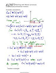

![MATH 1500 Sample Questions Exam 2 1. [3.7] A 10-ft plank is ...](https://img.yumpu.com/43861920/1/190x245/math-1500-sample-questions-exam-2-1-37-a-10-ft-plank-is-.jpg?quality=85)