Summary - Project Links - Rensselaer Polytechnic Institute
Summary - Project Links - Rensselaer Polytechnic Institute
Summary - Project Links - Rensselaer Polytechnic Institute

You also want an ePaper? Increase the reach of your titles
YUMPU automatically turns print PDFs into web optimized ePapers that Google loves.
UMAP<br />
The<br />
Journal<br />
Publisher<br />
COMAP, Inc. Vol. 30, No. 3<br />
Executive Publisher<br />
Solomon A. Garfunkel<br />
ILAP Editor<br />
Chris Arney<br />
Associate Director,<br />
Mathematics Division<br />
Program Manager,<br />
Cooperative Systems<br />
Army Research Office<br />
P.O. Box 12211<br />
Research Triangle Park,<br />
NC 27709-2211<br />
david.arney1@arl.army.mil<br />
On Jargon Editor<br />
Yves Nievergelt<br />
Dept. of Mathematics<br />
Eastern Washington Univ.<br />
Cheney, WA 99004<br />
ynievergelt@ewu.edu<br />
Reviews Editor<br />
James M. Cargal<br />
Mathematics Dept.<br />
Troy University—<br />
Montgomery Campus<br />
231 Montgomery St.<br />
Montgomery, AL 36104<br />
jmcargal@sprintmail.com<br />
Chief Operating Officer<br />
Laurie W. Aragón<br />
Production Manager<br />
George W. Ward<br />
Production Editor<br />
Joyce Barnes<br />
Distribution<br />
John Tomicek<br />
Graphic Designer<br />
Daiva Chauhan<br />
Editor<br />
Paul J. Campbell<br />
Beloit College<br />
700 College St.<br />
Beloit, WI 53511–5595<br />
campbell@beloit.edu<br />
Associate Editors<br />
Don Adolphson<br />
Chris Arney<br />
Aaron Archer<br />
Ron Barnes<br />
Arthur Benjamin<br />
Robert Bosch<br />
James M. Cargal<br />
Murray K. Clayton<br />
Lisette De Pillis<br />
James P. Fink<br />
Solomon A. Garfunkel<br />
William B. Gearhart<br />
William C. Giauque<br />
Richard Haberman<br />
Jon Jacobsen<br />
Walter Meyer<br />
Yves Nievergelt<br />
Michael O’Leary<br />
Catherine A. Roberts<br />
John S. Robertson<br />
Philip D. Straffin<br />
J.T. Sutcliffe<br />
Brigham Young Univ.<br />
Army Research Office<br />
AT&T Shannon Res. Lab.<br />
U. of Houston—Downtn<br />
Harvey Mudd College<br />
Oberlin College<br />
Troy U.— Montgomery<br />
U. of Wisc.—Madison<br />
Harvey Mudd College<br />
Gettysburg College<br />
COMAP, Inc.<br />
Calif. State U., Fullerton<br />
Brigham Young Univ.<br />
Southern Methodist U.<br />
Harvey Mudd College<br />
Adelphi University<br />
Eastern Washington U.<br />
Towson University<br />
College of the Holy Cross<br />
Georgia Military College<br />
Beloit College<br />
St. Mark’s School, Dallas
Subscription Rates for 2009 Calendar Year: Volume 30<br />
Institutional Web Membership (Web Only)<br />
Institutional Web Memberships do not provide print materials. Web memberships allow<br />
members to search our online catalog, download COMAP print materials, and reproduce<br />
them for classroom use.<br />
(Domestic) #2930 $467 (Outside U.S.) #2930 $467<br />
Institutional Membership (Print Only)<br />
Institutional Memberships receive print copies of The UMAP Journal quarterly, our<br />
annual CD collection of UMAP Modules, Tools for Teaching, and our organizational<br />
newsletter Consortium.<br />
(Domestic) #2940 $312 (Outside U.S.) #2941 $351<br />
Institutional Plus Membership (Print Plus Web)<br />
Institutional Plus Memberships receive print copies of the quarterly issues of The UMAP<br />
Journal, our annual CD collection of UMAP Modules, Tools for Teaching, our organizational<br />
newsletter Consortium, and online membership that allows members to search<br />
our online catalog, download COMAP print materials, and reproduce them for classroom<br />
use.<br />
(Domestic) #2970 $615 (Outside U.S.) #2971 $659<br />
For individual membership options visit<br />
www.comap.com for more information.<br />
To order, send a check or money order to COMAP, or call toll-free<br />
1-800-77-COMAP (1-800-772-6627).<br />
The UMAP Journal is published quarterly by the Consortium for Mathematics and Its<br />
Applications (COMAP), Inc., Suite 3B, 175 Middlesex Tpke., Bedford, MA, 01730, in<br />
cooperation with the American Mathematical Association of Two-Year Colleges<br />
(AMATYC), the Mathematical Association of America (MAA), the National Council of<br />
Teachers of Mathematics (NCTM), the American Statistical Association (ASA), the<br />
Society for Industrial and Applied Mathematics (SIAM), and The <strong>Institute</strong> for Operations<br />
Research and the Management Sciences (INFORMS). The Journal acquaints readers<br />
with a wide variety of professional applications of the mathematical sciences and<br />
provides a forum for the discussion of new directions in mathematical education<br />
(ISSN 0197-3622).<br />
Periodical rate postage paid at Boston, MA and at additional mailing offices.<br />
Send address changes to: info@comap.com<br />
COMAP, Inc., Suite 3B, 175 Middlesex Tpke., Bedford, MA, 01730<br />
© Copyright 2009 by COMAP, Inc. All rights reserved.<br />
Mathematical Contest in Modeling (MCM) ® , High School Mathematical Contest in<br />
Modeling (HiMCM) ® , and Interdisciplinary Contest in Modeling (ICM) ®<br />
are registered trade marks of COMAP, Inc.
Vol. 30, No. 3 2009<br />
Table of Contents<br />
Publisher’s Editorial<br />
The Faffufnik–Chaim Yankel Effect<br />
Solomon Garfunkel............................................................ 185<br />
About This Issue ................................................. 188<br />
Special Section on the MCM<br />
Results of the 2009 Mathematical Contest in Modeling<br />
Frank Giordano ................................................................ 189<br />
Abstracts of the Outstanding Papers ................................. 207<br />
A Simulation-Based Assessment of Traffic Circle Control<br />
Christopher Chang, Zhou Fan, and Yi Sun .......................... 227<br />
One Ring to Rule Them All: The Optimization of<br />
Traffic Circles<br />
Aaron Abromowitz, Andrea Levy, and Russell Melick ......... 247<br />
Three Steps to Make the Traffic Circle Go Round<br />
Zeyuan Allen Zhu, Tianyi Mao, and Yichen Huang ............. 261<br />
Pseudo-Finite Jackson Networks and Simulation:<br />
A Roundabout Approach to Traffic Control<br />
Anna Lieb, Anil Damle, and Geoffrey Peterson ................... 281<br />
Judges Commentary: The Outstanding Traffic Circle<br />
Papers<br />
Kelly Black ....................................................................... 305
Mobile to Mobil: The Primary Energy Costs for<br />
Cellular and Landline Telephones<br />
Nevin Brackett-Rozinsky, Katelynn Wilton, and<br />
Jason Altieri ...................................................................... 313<br />
Energy Implications of Cellular Proliferation<br />
in the U.S.<br />
Benjamin Coate, Zachary Kopplin, and Nate Landis ............ 333<br />
Modeling Telephony Energy Consumption<br />
Amrish Deshmukh, Rudolf Nikolaus Stahl, and<br />
Matthew Guay .................................................................. 353<br />
America’s New Calling<br />
Stephen R. Foster, J. Thomas Rogers, and Robert S. Potter .... 367<br />
Wireless Networks: An Easy Cell<br />
Jeff Bosco, Zachary Ulissi, and Bob Liu ............................... 385<br />
Judges’ Commentary: The Outstanding Cellphone<br />
Energy Papers<br />
Marie Vanisko ................................................................... 403<br />
Judges’ Commentary: The Fusaro Award for the<br />
Cellphone Energy Problem<br />
Marie Vanisko and Peter Anspach ......................................409
Publisher’s Editorial<br />
Publisher’s Editorial 185<br />
The Faffufnik–Chaim Yankel Effect<br />
Solomon A. Garfunkel<br />
Executive Director<br />
COMAP, Inc.<br />
175 Middlesex Turnpike, Suite 3B<br />
Bedford , MA 01730–1459<br />
s.garfunkel@mail.comap.com<br />
In the United States, as in many countries and more global entities, in<br />
order to receive funding for a major project, one has to submit a proposal. As<br />
anyone who has ever written one knows, writing a proposal is an unnatural<br />
act. Normally literate persons are reduced to using words such as “input”<br />
as a verb, as well as “facilitating” and “orientating,” and talking about<br />
“stakeholders” and “meta-cognition.” But large projects often require large<br />
budgets, and as painful as the process may be, we write the proposals and<br />
fill out the myriad forms required.<br />
Most of the money that comes from federal sources in the United States<br />
for math education projects is given in grants from the National Science<br />
Foundation (NSF). NSF uses a peer-review process to determine which<br />
projects are funded. Panels of approximately six people are formed to<br />
review a set of proposals. The proposals in each panel are graded and<br />
compared with the grades from several other panels that are convened at<br />
the same time. The programs are ordered by grade, and funding proceeds<br />
on that basis. What actually happens is that on a first pass, a number of<br />
projects are graded highly enough to be assured of funding; a number are<br />
graded so low that they are immediately declined; and there is a group in<br />
the middle (said to be “on the bubble”) whose fate is decided some time<br />
later when the final yearly budget for these programs is negotiated. The<br />
criteria for reviewing proposals, as specifically cited in NSF guidelines, are<br />
“intellectual merit” and “broader impacts.”<br />
The Consortium for Mathematics and Its Applications (COMAP) has<br />
been submitting proposals and administering projects for over 29 years. In<br />
the “good old days,” if one had a good idea and a good staff of people to<br />
carry out that idea, then funding usually depended upon impressing one of<br />
The UMAP Journal 30 (3) (2009) 185–188. c○Copyright 2009 by COMAP, Inc. All rights reserved.<br />
Permission to make digital or hard copies of part or all of this work for personal or classroom use<br />
is granted without fee provided that copies are not made or distributed for profit or commercial<br />
advantage and that copies bear this notice. Abstracting with credit is permitted, but copyrights<br />
for components of this work owned by others than COMAP must be honored. To copy otherwise,<br />
to republish, to post on servers, or to redistribute to lists requires prior permission from COMAP.
186 The UMAP Journal 30.3 (2009)<br />
the program officers who worked at the Foundation. Outside reviews were<br />
mostly handled by mail and were considered advisory. The bottom line was<br />
that if the NSF program officer thought that a project should be funded, it<br />
was. Admittedly, this created something of an old-boy network. People<br />
and institutions with a good track record of success tended to continue to<br />
receive funding, while those who were not yet members of the club had<br />
a hard time joining. This has given way to the more overtly democratic<br />
process described above where the reviewers’ opinions rule.<br />
It should also be said that if one goes back 20 years or so, most of the<br />
principal investigators (PIs) on mathematics education projects were Ph.D.<br />
mathematicians who had, so to speak, “given their youth to the devil and<br />
were giving their old age to the Lord.” In other words, they had taken<br />
an interest in mathematics education later in their careers. And, to be<br />
honest, many other mathematics educators were persons who originally<br />
pursued careers as research mathematicians but were unable to complete<br />
their degrees. In any event, the PIs on these projects had extremely strong<br />
mathematics backgrounds.<br />
In the United States at least, this has changed significantly. Mathematics<br />
education is now a well-established field unto itself and, in many cases,<br />
people highly successful in the field have relatively weak mathematical<br />
training. Increasingly, they are the principal investigators on new projects<br />
in mathematics education and they are the reviewers. They help decide<br />
what projects get funded and what projects don’t. And, increasingly, they<br />
are responsible for the Faffufnik–ChaimYankel Effect (FCE). What exactly is<br />
the FCE?<br />
Years ago, a typical review of a COMAP proposal would read, “This is<br />
an excellent idea with an excellent staff with an excellent track record; we<br />
recommend this project for funding.” The FCE refers to more typical current<br />
reviews that read, “This is an excellent idea with an excellent staff with an<br />
excellent track record. However, we have to recommend against funding<br />
because they don’t make any reference to the seminal research papers of<br />
Faffufnik, nor do they plan to use the statistical protocols of Chaim Yankel.”<br />
The reviewers may very well be students of Faffufnik and/or Chaim Yankel.<br />
Of course, there are some sour grapes here. I am not a member of the<br />
Faffufnik and Chaim Yankel club. And now, as opposed to the good old<br />
days, it is the members of this club who get funded. But there is much<br />
more to be discussed. There appears to be an underlying assumption that<br />
mathematics education projects must proceed in the following way.<br />
• First, they must be based upon research. Therefore, we heavily quote the<br />
results of prior research (see the papers of Faffufnik).<br />
• Then, based upon that research, we make a new research hypothesis and<br />
test it with a small number of students. If at all possible, we make this<br />
experiment as close to a “gold standard” double-blind medical approach<br />
as possible.
Publisher’s Editorial 187<br />
• Then, using certain statistical protocols (see the work of Chaim Yankel),<br />
we conclude that there is some measurable effect and write a new proposal<br />
to test this effect on a larger population.<br />
• This process is then iterated.<br />
This is now a necessary condition for funding—independent of content and<br />
the strength of the ideas being considered.<br />
The problem is that while this may very well help to make mathematics<br />
education research be seen as more of an established discipline, it is a criterion<br />
divorced from classroom practice. And we forget that we separate<br />
our efforts in education from the classroom at our peril. There has to be a<br />
way for good ideas that hold the promise of increasing student learning to<br />
be funded and for good people to work on them. Mathematics education<br />
is an art as well as a science, and it cannot be reduced to a set of research<br />
protocols and statistical tests and procedures. It is simply not possible to<br />
prove that an approach to teaching and learning will be effective before the<br />
fact.<br />
Education, as a scientific discipline, is a young field with an active community<br />
focused on R&D—research on learning coupled with the development<br />
of new and better curriculum materials. In truth, however, much<br />
of the work is better described as D&R—informed and thoughtful development<br />
followed by careful analysis of results. It is in the nature of the<br />
enterprise that we cannot discover what works before we create the what.<br />
Curriculum development, in particular, is best related to an engineering<br />
paradigm. To test the efficacy of an approach, we must analyze needs, examine<br />
existing programs, build an improved model program, and then test<br />
it—in the same way that we build scale models to design a better bridge or<br />
building. This kind of iterative D&R leads to new and more effective materials<br />
and new pedagogical approaches that better incorporate the growing<br />
body of knowledge of cognitive science.<br />
I wish to be clear. I recognize that Faffufnik has done important research.<br />
I recognize that Chaim Yankel’s protocols can help quantify our<br />
results. We must learn from the past, and theoretical frameworks are important<br />
for future work. But we also must recognize that quoting Faffufnik<br />
and ChaimYankel is not a substitute for imagination, creativity, and the<br />
application of common sense. The problems of mathematics education are<br />
difficult and will require the work of many people over a long period of<br />
time. We cannot afford to lose sight of this, even as mathematics education<br />
becomes a more-established research discipline.<br />
Acknowledgment<br />
This editorial is adapted from the author’s talk at the International Commission<br />
on Mathematical Instruction (ICMI) meeting in Rome, Italy, 2008.
188 The UMAP Journal 30.3 (2009)<br />
About the Author<br />
Solomon Garfunkel, previously of Cornell University and the University<br />
of Connecticut at Storrs, has dedicated the last 30 years to research and<br />
development efforts in mathematics education. He has served as project<br />
director for the Undergraduate Mathematics and Its Applications (UMAP)<br />
and the High School Mathematics and Its Applications (HiMAP) <strong>Project</strong>s<br />
funded by NSF, and directed three telecourse projects including Against All<br />
Odds: Inside Statistics, and In Simplest Terms: College Algebra, for the Annenberg/CPB<br />
<strong>Project</strong>. He has been the Executive Director of COMAP, Inc.<br />
since its inception in 1980. Dr. Garfunkel was the project director and host<br />
for the series, For All Practical Purposes: Introduction to Contemporary Mathematics.<br />
He was the Co-Principal Investigator on the ARISE <strong>Project</strong>, and is<br />
currently the Co-Principal Investigator of the CourseMap, ResourceMap,<br />
and WorkMap projects. In 2003, Dr. Garfunkel was Chair of the National<br />
Academy of Sciences and Mathematical Sciences Education Board Committee<br />
on the Preparation of High School Teachers.<br />
About This Issue<br />
Paul J. Campbell<br />
Editor<br />
This issue runs longer than a regular 92-page issue, to more than 200<br />
pages. However, not all of the articles appear in the paper version. Some<br />
appear only on the Tools for Teaching 2009 CD-ROM (and at http://www.<br />
comap.com for COMAP members), which will reach members and subscribers<br />
later and will also contain the entire 2009 year of Journal issues.<br />
All articles listed in the table of contents are regarded as published in<br />
the Journal. The abstract of each appears in the paper version. Pagination<br />
of the issue runs continuously, including in sequence articles that do not<br />
appear in the paper version. So if, say, p. 250 in the paper version is followed<br />
by p. 303, your copy is not necessarily defective! The articles on the intervening<br />
pages are on the CD-ROM.<br />
We hope that you find this arrangement agreeable. It means that we do<br />
not have to procrusteanize the content to fit a fixed number of paper pages.<br />
We might otherwise be forced to select only two or three Outstanding MCM<br />
papers to publish. Instead, we continue to bring you the full content.
Modeling Forum<br />
Results of the 2009 MCM 189<br />
Results of the 2009<br />
Mathematical Contest in Modeling<br />
Frank Giordano, MCM Director<br />
Naval Postgraduate School<br />
1 University Circle<br />
Monterey, CA 93943-5000<br />
fgiordano@nps.edu<br />
Introduction<br />
A total of 1,675 teams of undergraduates from hundreds of institutions and<br />
departments in 14 countries, spent the first weekend in February working on<br />
applied mathematics problems in the 25th Mathematical Contest in Modeling.<br />
The 2009 Mathematical Contest in Modeling (MCM) began at 8:00 P.M. EST<br />
on Thursday, February 5 and ended at 8:00 P.M. EST on Monday, February 9.<br />
During that time, teams of up to three undergraduates researched, modeled,<br />
and submitted a solution to one of two open-ended modeling problems. Students<br />
registered, obtainedcontest materials, downloadedthe problem and data,<br />
and entered completion data through COMAP’s MCM Website. After a weekend<br />
of hard work, solution papers were sent to COMAP on Monday. The top<br />
papers appear in this issue of The UMAP Journal, together with commentaries.<br />
In addition to this special issue of The UMAP Journal, this year—for the<br />
first time—COMAP has made available a special supplementary “2009 MCM-<br />
ICM CD-ROM” containing the press releases for the two contests, the results,<br />
the problems, and original versions of the Outstanding papers that appear<br />
here in edited form. Information about ordering the CD-ROM is at http:<br />
//www.comap.com/product/?idx=1025 or from (800) 772–6627.<br />
Results and winning papers from the first 24 contests were published in<br />
special issues of Mathematical Modeling (1985–1987) and The UMAP Journal<br />
(1985–2008). The 1994 volume of Tools for Teaching, commemorating the tenth<br />
anniversary of the contest, contains the 20 problems used in the first 10 years<br />
of the contest and a winning paper for each year. That volume and the special<br />
The UMAP Journal 30 (3) (2009) 189–206. c○Copyright 2009 by COMAP, Inc. All rights reserved.<br />
Permission to make digital or hard copies of part or all of this work for personal or classroom use<br />
is granted without fee provided that copies are not made or distributed for profit or commercial<br />
advantage and that copies bear this notice. Abstracting with credit is permitted, but copyrights<br />
for components of this work owned by others than COMAP must be honored. To copy otherwise,<br />
to republish, to post on servers, or to redistribute to lists requires prior permission from COMAP.
190 The UMAP Journal 30.3 (2009)<br />
MCM issues of the Journal for the last few years are available from COMAP. The<br />
1994 volume is also available on COMAP’s special Modeling Resource CD-ROM.<br />
Also available is The MCM at 21 CD-ROM, which contains the 20 problems<br />
from the second 10 years of the contest, a winning paper from each year, and<br />
advice from advisors of Outstanding teams. These CD-ROMs can be ordered<br />
from COMAP at http://www.comap.com/product/cdrom/index.html .<br />
This year, the two MCM problems represented significant challenges. The<br />
author of Problem A, Daniel Solow of Case Western Reserve University, Cleveland,<br />
OH, was also one of the final judges. His problem, “Designing a Traffic<br />
Circle,” asked teams to use a model to determine how best to control traffic flow<br />
in, around, and out of a circle, clearly stating the objective(s) and summarizing<br />
the conditions for use of various types of traffic-control methods. Problem B,<br />
“Energy and the Cellphone,” was written by Joe Malkevitch of York College<br />
in Jamaica, NY. What is the long-term consequence of large-scale usage of cellphones<br />
in terms of electricity use by the battery and the charger? Teams were<br />
asked to take into account the fact that cellphones last much less time (they get<br />
lost and break) than phones for landlines and to suggest an optimal way (in<br />
terms of an energy perspective) to provide phone service to a “Pseudo U.S.,”<br />
a country of 300 million people with about the same economic status as the<br />
current U.S. but with no landlines or cellphones.<br />
In addition to the MCM, COMAP also sponsors the Interdisciplinary Contest<br />
in Modeling (ICM) and the High School Mathematical Contest in Modeling<br />
(HiMCM). The ICM runs concurrently with MCM and for the next several<br />
years will offer a modeling problem involving an environmental topic. Results<br />
of this year’s ICM are on the COMAP Website at http://www.comap.<br />
com/undergraduate/contests; results and Outstanding papers appeared<br />
in Vol. 30 (2009), No. 2. The HiMCM offers high school students a modeling<br />
opportunity similar to the MCM. Further details about the HiMCM are at<br />
http://www.comap.com/highschool/contests .<br />
2009 MCM Statistics<br />
• 1,675 teams participated<br />
• 7 high school teams (
• 1,074 Successful Participants (63%)<br />
Results of the 2009 MCM 191<br />
Problem A: Designing a Traffic Circle<br />
Many cities and communities have traffic circles—from large ones with<br />
many lanes in the circle (such as at the Arc de Triomphe in Paris and the Victory<br />
Monument in Bangkok) to small ones with one or two lanes in the circle. Some<br />
of these traffic circles position a stop sign or a yield sign on every incoming<br />
road, which gives priority to traffic already in the circle; some position a yield<br />
sign in the circle at each incoming road to give priority to incoming traffic; and<br />
some position a traffic light on each incoming road (with no right turn allowed<br />
on a red light). Other designs may also be possible.<br />
The goal of this problem is to use a model to determine how best to control<br />
traffic flow in, around, and out of a circle. State clearly the objective(s) you<br />
use in your model for making the optimal choice as well as the factors that<br />
affect this choice. Include a Technical <strong>Summary</strong> of not more than two doublespaced<br />
pages that explains to a traffic engineer how to use your model to help<br />
choose the appropriate flow-control method for any specific traffic circle. That<br />
is, summarize the conditions under which each type of traffic-control method<br />
should be used. When traffic lights are recommended, explain a method for<br />
determining how many seconds each light should remain green (which may<br />
vary according to the time of day and other factors). Illustrate how your model<br />
works with specific examples.<br />
Problem B: Energy and the Cellphone<br />
This question involves the “energy” consequences of the cellphone revolution.<br />
Cellphone usage is mushrooming, and many people are using cellphones<br />
and giving up their landline telephones. What is the consequence of this in<br />
terms of electricity use? Every cellphone comes with a battery and a recharger.<br />
Requirement 1<br />
Consider the current U.S., a country of about 300 million people. Estimate<br />
from available data the number H of households, with m members each, that<br />
in the past were serviced by landlines. Now, suppose that all the landlines are<br />
replaced by cellphones; that is, each of the m members of the household has a<br />
cellphone. Model the consequences of this change for electricity utilization in<br />
the current U.S., both during the transition and during the steady state. The<br />
analysis should take into account the need for charging the batteries of the<br />
cellphones, as well as the fact that cellphones do not last as long as landline<br />
phones (for example, the cellphones get lost and break).
192 The UMAP Journal 30.3 (2009)<br />
Requirement 2<br />
Consider a second “Pseudo U.S.”—a country of about 300 million people<br />
with about the same economic status as the current U.S. However, this emerging<br />
country has neither landlines nor cellphones. What is the optimal way of<br />
providing phone service to this country from an energy perspective? Of course,<br />
cellphones have many social consequences and uses that landline phones do<br />
not allow. A discussion of the broad and hidden consequences of having only<br />
landlines, only cellphones, or a mixture of the two is welcomed.<br />
Requirement 3<br />
Cellphones periodically need to be recharged. However, many people always<br />
keep their recharger plugged in. Additionally, many people charge their<br />
phones every night, whether they need to be recharged or not. Model the energy<br />
costs of this wasteful practice for a Pseudo U.S. based on your answer<br />
to Requirement 2. Assume that the Pseudo U.S. supplies electricity from oil.<br />
Interpret your results in terms of barrels of oil.<br />
Requirement 4<br />
Estimates vary on the amount of energy that is used by various recharger<br />
types (TV, DVR, computer peripherals, and so forth) when left plugged in but<br />
not charging the device. Use accurate data to model the energy wasted by the<br />
current U.S. in terms of barrels of oil per day.<br />
Requirement 5<br />
Now consider population and economic growth over the next 50 years.<br />
How might a typical Pseudo U.S. grow? For each 10 years for the next 50 years,<br />
predict the energy needs for providing phone service based upon your analysis<br />
in the first three requirements. Again, assume electricity is provided from oil.<br />
Interpret your predictions in term of barrels of oil.<br />
The Results<br />
The solution papers were coded at COMAP headquarters so that names and<br />
affiliations of the authors would be unknown to the judges. Each paper was<br />
then read preliminarily by two “triage” judges at either Appalachian State University<br />
(Traffic Circle Problem) or at the National Security Agency (Cellphone<br />
Energy Problem). At the triage stage, the summary and overall organization<br />
are the basis for judging a paper. If the judges’ scores diverged for a paper, the<br />
judges conferred; if they still did not agree, a third judge evaluated the paper.
Results of the 2009 MCM 193<br />
AdditionalRegionalJudgingsites were created at the U.S. MilitaryAcademy<br />
and at the Naval Postgraduate School to support the growing number of contest<br />
submissions.<br />
Final judging took place at the Naval Postgraduate School, Monterey, CA.<br />
The judges classified the papers as follows:<br />
Honorable Successful<br />
Outstanding Meritorious Mention Participation Total<br />
Traffic Circle Problem 4 192 165 763 1124<br />
Cellphone Energy Problem 5 102 133 311 551<br />
9 294 298 1074 1675<br />
The 9 papers that the judges designated as Outstanding appear in this special<br />
issue of The UMAP Journal, together with commentaries. We list those<br />
teams here and the Meritorious teams (and advisors) at the end of this report;<br />
the list of all participating schools, advisors, and results is in the Appendix.<br />
Outstanding Teams<br />
Institution and Advisor Team Members<br />
“A Simulation-Based Assessment<br />
of Traffic Circle Control”<br />
Harvard University<br />
Cambridge, MA<br />
Clifford H. Taubes<br />
Traffic Circle Papers<br />
“One Ring to Rule Them All:<br />
The Optimization of Traffic Circles”<br />
Harvey Mudd College<br />
Claremont, CA<br />
Susan E. Martonosi<br />
“Three Steps to Make the Traffic<br />
Circle Go Round”<br />
Tsinghua University<br />
Beijing, China<br />
Jun Ye<br />
Christopher Chang<br />
Zhou Fan<br />
Yi Sun<br />
Aaron Abromowitz<br />
Andrea Levyi<br />
Russell Melick<br />
Zeyuan Zhu<br />
Tianyi Mao<br />
Yichen Huang
194 The UMAP Journal 30.3 (2009)<br />
“Pseudo-Finite Jackson Networks and<br />
Simulation: A Roundabout<br />
Approach to Traffic Control”<br />
University of Colorado<br />
Boulder, CO<br />
Anne Dougherty<br />
Cellphone Energy Papers<br />
“Mobile to Mobil: The Primary Energy<br />
Costs for Cellular and Landline<br />
Telephones”<br />
Clarkson University<br />
Potsdam, NY<br />
Joseph Skufca<br />
“Energy Implications of Cellular<br />
Proliferation in the U.S.”<br />
College of Idaho<br />
Caldwell, IDA<br />
Michael P. Hitchman<br />
“Modeling Telephony Energy<br />
Consumption”<br />
Cornell University<br />
Ithaca, NY<br />
Alexander Vladimirsky<br />
“America’s New Calling”<br />
Southwestern University<br />
Georgetown, TX<br />
Richard Denman<br />
“Wireless Networks: An Easy Cell”<br />
University of Delaware<br />
Newark, DE<br />
Louis Rossi<br />
Anna Lieb<br />
Anil Damle<br />
Geoffrey Peterson<br />
Nevin Brackett-Rozinsky<br />
Katelynn Wilton<br />
Jason Altieri<br />
Benjamin Coate<br />
Zachary Kopplin<br />
Nate Landis<br />
Amrish Deshmukh<br />
Rudolf Nikolaus Stahl<br />
Matthew Guay<br />
Stephen R. Foster<br />
J. Thomas Rogers<br />
Robert S. Potter<br />
Jeff Bosco<br />
Zachary Ulissi<br />
Bob Liu
Awards and Contributions<br />
Results of the 2009 MCM 195<br />
Each participating MCM advisor and team member received a certificate<br />
signed by the Contest Director and the appropriate Head Judge.<br />
INFORMS, the <strong>Institute</strong> for Operations Research and the Management<br />
Sciences, recognized the teams from the University of Colorado–Boulder<br />
(Traffic Circle Problem) and Cornell University(CellphoneEnergy Problem)<br />
as INFORMS Outstanding teams and provided the following recognition:<br />
• a letter of congratulations from the current president of INFORMS to<br />
each team member and to the faculty advisor;<br />
• a check in the amount of $300 to each team member;<br />
• a bronze plaque for display at the team’s institution, commemorating<br />
their achievement;<br />
• individual certificates for team members and faculty advisor as a personal<br />
commemoration of this achievement;<br />
• a one-year student membership in INFORMS for each team member,<br />
which includes their choice of a professional journal plus the OR/MS<br />
Today periodical and the INFORMS society newsletter.<br />
The Society for Industrial and Applied Mathematics (SIAM) designated<br />
one Outstanding team from each problem as a SIAM Winner. The teams<br />
were from Harvard University (Traffic Circle Problem) and Southwestern<br />
University (Cellphone Energy Problem). Each of the team members was<br />
awarded a $300 cash prize, and the teams received partial expenses to<br />
present their results in a special Minisymposium at the SIAM Annual Meeting<br />
in Denver, CO in July. Their schools were given a framed hand-lettered<br />
certificate in gold leaf.<br />
The Mathematical Association of America (MAA) designated one Outstanding<br />
North American team from each problem as an MAA Winner. The<br />
teams were from Harvey Mudd College (Traffic Circle Problem) and Clarkson<br />
University (Cellphone Energy Problem). With partial travel support<br />
from the MAA, the teams presented their solution at a special session of the<br />
MAA Mathfest in Portland, OR in August. Each team member was presented<br />
a certificate by an official of the MAA Committee on Undergraduate<br />
Student Activities and Chapters.<br />
Ben Fusaro Award<br />
One Meritorious or Outstanding paper was selected for each problem for<br />
the Ben Fusaro Award, named for the Founding Director of the MCM and<br />
awarded for the sixth time this year. It recognizes an especially creative<br />
approach; details concerning the award, its judging, and Ben Fusaro are<br />
in Vol. 25 (3) (2004): 195–196. The Ben Fusaro Award winners were the
196 The UMAP Journal 30.3 (2009)<br />
University of Iowa (Traffic Circle Problem) and Lawrence Technological<br />
University (Cellphone Energy Problem).<br />
Judging<br />
Director<br />
Frank R. Giordano, Naval Postgraduate School, Monterey, CA<br />
Associate Director<br />
William P. Fox, Dept. of Defense Analysis, Naval Postgraduate School,<br />
Monterey, CA<br />
Traffic Circle Problem<br />
Head Judge<br />
Marvin S. Keener, Executive Vice-President, Oklahoma State University,<br />
Stillwater, OK<br />
Associate Judges<br />
William C. Bauldry, Chair, Dept. of Mathematical Sciences,<br />
Appalachian State University, Boone, NC (Head Triage Judge)<br />
Kelly Black, Mathematics Dept., Union College, Schenectady, NY<br />
Karen D. Bolinger, Mathematics Dept., Clarion University of Pennsylvania,<br />
Clarion, PA (SIAM Judge)<br />
Patrick J. Driscoll, Dept. of Systems Engineering, U.S. Military Academy,<br />
West Point, NY<br />
J. Douglas Faires, Youngstown State University, Youngstown, OH<br />
Ben Fusaro, Dept. of Mathematics, Florida State University, Tallahassee, FL<br />
Jerry Griggs, Mathematics Dept., University of South Carolina, Columbia,<br />
SC (Problem Author)<br />
Steve Horton, Dept. of Mathematical Sciences, U.S. Military Academy,<br />
West Point, NY (MAA Judge)<br />
Mario Juncosa, RAND Corporation, Santa Monica, CA (retired)<br />
Michael Moody, Olin College of Engineering, Needham, MA (SIAM Judge)<br />
John L. Scharf, Mathematics Dept., Carroll College, Helena, MT<br />
(Ben Fusaro Award Judge)<br />
Dan Solow, Mathematics Dept., Case Western Reserve University,<br />
Cleveland, OH (INFORMS Judge)<br />
Michael Tortorella, Dept. of Industrial and Systems Engineering,<br />
Rutgers University, Piscataway, NJ<br />
Richard Douglas West, Francis Marion University, Florence, SC<br />
Dan Zwillinger, Raytheon Company, Sudbury, MA
Results of the 2009 MCM 197<br />
Cellphone Energy Problem<br />
Head Judge<br />
Maynard Thompson, Mathematics Dept., University of Indiana,<br />
Bloomington, IN<br />
Associate Judges<br />
Peter Anspach, National Security Agency, Ft. Meade, MD<br />
(Head Triage Judge)<br />
Jim Case (SIAM Judge)<br />
Veena Mendiratta, Lucent Technologies, Naperville, IL<br />
Peter Olsen, Johns Hopkins Applied Physics Laboratory, Baltimore, MD<br />
David H. Olwell, Naval Postgraduate School, Monterey, CA<br />
(INFORMS Judge)<br />
Kathleen M. Shannon, Dept. of Mathematics and Computer Science,<br />
Salisbury University, Salisbury, MD (SIAM Judge)<br />
Marie Vanisko, Dept. of Mathematics, Carroll College, Helena, MT<br />
(Ben Fusaro Award Judge)<br />
Regional Judging Session at U.S. Military Academy<br />
Head Judges<br />
Patrick J. Driscoll, Dept. of Systems Engineering, and<br />
Steve Horton, Dept. of Mathematical Sciences,<br />
United States Military Academy (USMA), West Point, NY<br />
Associate Judges<br />
Tim Elkins, Dept. of Systems Engineering, USMA<br />
Michael Jaye, Dept. of Mathematical Sciences, USMA<br />
Darrall Henderson, Sphere Consulting, LLC<br />
Steve Horton, Dept. of Mathematical Sciences, USMA<br />
Tom Meyer, Dept. of Mathematical Sciences, USMA<br />
Scott Nestler, Dept. of Mathematical Sciences, USMA<br />
Regional Judging Session at Naval Postgraduate School<br />
Head Judge<br />
William P. Fox, Dept. of Defense Analysis, and Frank Giordano,<br />
Naval Postgraduate School (NPS), Monterey, CA<br />
Associate Judges<br />
Greg Mislik, Matt Boensel, and Pete Gustitis<br />
—all from the Naval Postgraduate School, Monterey, CA<br />
Triage Session for Traffic Circle Problem<br />
Head Triage Judge<br />
William C. Bauldry, Chair, Dept. of Mathematical Sciences,<br />
Appalachian State University, Boone, NC
198 The UMAP Journal 30.3 (2009)<br />
Associate Judges<br />
Jeffry Hirst, Rick Klima, Mark Ginn, and Tracie McLemore Salinas<br />
—all from Dept. of Mathematical Sciences, Appalachian State University,<br />
Boone, NC<br />
Triage Session for Cellphone Energy Problem<br />
Head Triage Judges<br />
Peter Anspach, National Security Agency (NSA), Ft. Meade, MD<br />
Jim Case<br />
Associate Judges<br />
Other judges from inside and outside NSA, who wish not to be named.<br />
Sources of the Problems<br />
The Traffic Circle Problem was contributed by Daniel Solow (Case Western<br />
Reserve University), who was also one of the final judges, and the<br />
Cellphone Energy Problem by Joe Malkevitch (York College of CUNY).<br />
Acknowledgments<br />
Major funding for the MCM is provided by the National Security Agency<br />
(NSA) and by COMAP. Additional support is provided by the <strong>Institute</strong> for<br />
Operations Research and the Management Sciences (INFORMS), the Society<br />
for Industrial and Applied Mathematics (SIAM), and the Mathematical<br />
Association of America (MAA). We are indebted to these organizations for<br />
providing judges and prizes.<br />
We also thank for their involvement and support the MCM judges and<br />
MCM Board members for their valuable and unflagging efforts, as well as<br />
• Two Sigma Investments. (This group of experienced, analytical, and<br />
technical financial professionals based in New York builds and operates<br />
sophisticated quantitative trading strategies for domestic and international<br />
markets. The firm is successfully managing several billion dollars<br />
using highly automated trading technologies. For more information<br />
about Two Sigma, please visit http://www.twosigma.com .)
Cautions<br />
Results of the 2009 MCM 199<br />
To the reader of research journals:<br />
Usually a published paper has been presented to an audience, shown<br />
to colleagues, rewritten, checked by referees, revised, and edited by a journal<br />
editor. Each paper here is the result of undergraduates working on<br />
a problem over a weekend. Editing (and usually substantial cutting) has<br />
taken place; minor errors have been corrected, wording altered for clarity<br />
or economy, and style adjusted to that of The UMAP Journal. The student<br />
authors have proofed the results. Please peruse their efforts in that context.<br />
To the potential MCM Advisor:<br />
It might be overpowering to encounter such output from a weekend<br />
of work by a small team of undergraduates, but these solution papers are<br />
highly atypical. A team that prepares and participates will have an enriching<br />
learning experience, independent of what any other team does.<br />
COMAP’sMathematicalContest in Modelingand InterdisciplinaryContest<br />
in Modeling are the only international modeling contests in which<br />
students work in teams. Centering its educational philosophy on mathematical<br />
modeling, COMAP uses mathematical tools to explore real-world<br />
problems. It serves the educational community as well as the world of work<br />
by preparing students to become better-informed and better-prepared citizens.<br />
Meritorious Teams<br />
Designations of departments named Mathematics, Mathematical Sciences, Mathematics and<br />
Computer Science, or the like are omitted.<br />
Traffic Circle Problem (192 teams)<br />
Beihang University, Beijing, China (Peng Lin Ping)<br />
Beihang University, Advanced Engineering, Beijing, China (Wei Feng)<br />
Beijing <strong>Institute</strong> of Technology, Beijing, China (Xue-Wen Li)<br />
Beijing <strong>Institute</strong> of Technology, Beijing, China (Gui-Feng Yan)<br />
Beijing <strong>Institute</strong> of Technology, Beijing, China (Chun-guang Xiong)<br />
Beijing <strong>Institute</strong> of Technology, Beijing, China (Bing-Zhao Li)<br />
Beijing Jiaotong University, Beijing, China (Bingtuan Wang)<br />
Beijing Jiaotong University, Beijing, China (Peng Cao)<br />
Beijing Language and Culture University, Computer Science, Beijing, China (Xiaoxia Zhao)<br />
Beijing Language and Culture University, Computer Science, Beijing, China (Ping Yang)<br />
Beijing Normal University, Beijing, China (Qing He)<br />
Beijing Normal University, Beijing, China (Xianghui Shi)<br />
Beijing University of Posts and Telecommunications, Computer Science and Technology, Beijing,<br />
China (Wenbo Zhang)
200 The UMAP Journal 30.3 (2009)<br />
Beijing University of Posts and Telecommunications, Electronic Engineering, Beijing, China<br />
(Qing Zhou)<br />
Beijing University of Posts and Telecommunications, Electronic Engineering, Beijing, China<br />
(Jianhua Yuan)<br />
Bethel University, Arden Hills, MN (Nathan M. Gossett) (two teams)<br />
Bucknell University, Lewisburg, PA (Nathan, C. Ryan)<br />
Carnegie Mellon University, Pittsburgh, PA (Dale J. Winter)<br />
Carroll College, Natural Sciences, Helena, MT (Anthony Szpilka)<br />
Carroll College, Mathematics, Engineering, and Computer Science, Helena, MT<br />
(Jack Oberweiser)<br />
Central China Normal University, Mathematics and Statistics Department, Wuhan, Hubei, China<br />
(Bo Li)<br />
Central South University, Metallurgical Science and Engineering, Changsha, Hunan, China<br />
(Muzhou Hou)<br />
Central South University, Mathematics and Applied Mathematics, Changsha, Hunan, China<br />
(Zheng Zhoushun)<br />
Central University of Finance and Economics, Applied Mathematics, Beijing, China<br />
(Huiqing Huang)<br />
Central Washington University, Ellensburg WA (James W. Bisgard)<br />
Chengdu University of Technology, Information Management, Chengdu, Sichuan, China<br />
(YouHua Wei)<br />
China University of Petroleum, Dongying, Shandong, China (Xinhai Liu)<br />
China University of Petroleum–Beijing, Mathematics and Physics, Beijing, China (Ling Zhao)<br />
Chinese University of Hong Kong, Physics, Hong Kong, China (Ming Chung Chu)<br />
City University of Hong Kong, Hong Kong, China (Jonathan J. Wylie)<br />
Clarion University, Clarion, PA (David M. Hipfel)<br />
Clarkson University, Computer Science, Potsdam, NY (Kathleen R. Fowler) (two teams)<br />
Coe College, Cedar Rapids, IA (Jonathan White)<br />
College of Charleston, Charleston, SC (William G. Mitchener) (two teams)<br />
Colorado College, Colorado Springs, CO (Amelia Taylor)<br />
Cornell University, Ithaca, NY (Alexander Vladimirsky)<br />
Dalian Maritime University, Dalian, Liaoning, China (Naxin Chen)<br />
Dalian Maritime University, Dalian, Liaoning, China (Xiangpeng Kong) (two teams)<br />
Dalian University of Technology, Software, Dalian, Liaoning, China (Ning Ding)<br />
Dalian University of Technology, Software, Dalian, Liaoning, China (Tie Qiu)<br />
Dalian University of Technology, Applied Mathematics, Dalian, Liaoning, China (Mingfeng He)<br />
Dalian University of Technology, Applied Mathematica, Dalian, Liaoning, China (Qiuhui Pan)<br />
Dalian University of Technology, Innovation Experiment, Dalian, Liaoning, China (Lin Feng)<br />
Davidson College, Davidson, NC (Tim Chartier)<br />
East China Normal University, Statistics and Actuarial Science, Shanghai, China (Shujin Wu)<br />
Eastern Michigan University, Ypsilanti, MI (Andrew M. Ross)<br />
Fudan University, Shanghai, China (Zhijie Cai)<br />
Fujian Normal University, Fuzhou, Fujian, China (Qinghua Chen)<br />
Fujian Normal University, Fuzhou, Fujian, China (Changfeng Ma)<br />
Guangdong University of Business Studies, Guangzhou, Guangdong, China (Zigui Xiang)<br />
Hangzhou Dianzi University, Information and Mathematical Science, Hangzhou, Zhejiang, China<br />
(Hao Shen)<br />
Harbin Engineering University, Science, Harbin, Heilongjiang, China (Zhenbin Gao)<br />
Harbin Engineering University, Science, Harbin, Heilongjiang, China (Dongqi Sun)
Results of the 2009 MCM 201<br />
Harbin <strong>Institute</strong> of Technology, Harbin, Heilongjiang, China (Guofeng Fan) (two teams)<br />
Harbin <strong>Institute</strong> of Technology, Computer Science, Harbin, Heilongjiang, China (Zheng Kuang)<br />
Harbin <strong>Institute</strong> of Technology, Automatic Measurement and Control, Harbin, Heilongjiang, China<br />
(Limin Zou)<br />
Harbin <strong>Institute</strong> of Technology, Weihai, Shandong, China (Rongning Qu)<br />
Harbin University of Science and Technology, Harbin, Heilongjiang, China (Fengqiu Liu)<br />
Harvard University, Engineering and Applied Sciences, Cambridge, MA<br />
(Michael Brenner)<br />
Harvey Mudd College, Claremont, CA (Rachel Levy)<br />
Harvey Mudd College, Claremont, CA (Francis Su)<br />
Huazhong University of Science and Technology, Mathematics and Statistics, Wuhan, Hubei, China<br />
(Zhihong Lu)<br />
Jiangsu University, Zhenjiang, Jiangsu, China (Yang Hong Lin)<br />
Jilin University, Changchun, Jilin, China (Yongkui Zou)<br />
Lawrence Technological University, Southfield, MI (Ruth G. Favro)<br />
Lawrence University, Appleton, WI (Bruce H. Pourciau)<br />
Linfield College, McMinnville, OR (Martha E. VanCleave)<br />
Luther College, Computer Science, Decorah, IA (Steve Hubbard)<br />
Macquarie University, North Ryde, NSW, Australia (Xuan Duong)<br />
McGill University, Mathematics and Statistics, Montreal, QC, Canada (Bruce Shepherd)<br />
MIT, Cambridge, MA (Martin Zdenek Bazant)<br />
Mount St. Mary’s University, Emmitsburg, MD (Brian Heinold)<br />
Nanjing University, Computer Science and Technology, Nanjing, Jiangsu, China (Zhengxing Sun)<br />
Nanjing University, Nanjing, Jiangsu, China (Huang Wei Hua)<br />
Nanjing University of Posts and Telecommunications, Mathematics and Physics, Nanjing, Jiangsu,<br />
China (Jun Ye)<br />
National University of Defense Technology, Mathematics and System Science, Changsha, Hunan,<br />
China (Ziyang Mao)<br />
National University of Defense Technology, Department of Mathematics and System Science,<br />
Changsha, Hunan, China (Mengda Wu)<br />
National University of Singapore, Singapore (Hwee Huat Tan)<br />
National University of Singapore, Statistics and Applied Probability, Singapore (Wei-Liem Loh)<br />
North Carolina School of Science and Mathematics, Durham, NC (Daniel J. Teague) (two teams)<br />
Northeastern University, Information Science and Engineering, Shenyang, Liaoning, China<br />
(Dali Chen)<br />
Northeastern University, System Science, Shenyang, Liaoning, China (Xuefeng Zhang)<br />
Northwest University, Xi’an, Shaanxi, China (Liantang Wang)<br />
Oklahoma State University, Stillwater, OK (Benny Evans)<br />
Pacific Lutheran University, Tacoma, WA (Mei Zhu)<br />
Pacific University, Forest Grove, OR (Christine Guenther)<br />
Peking University, Computer Science, Beijing, China (Bo Peng)<br />
Peking University, Beijing, China (Shanjun Lin)<br />
Peking University, Beijing, China (Shanjun Lin)<br />
Peking University, Beijing, China (Xiang Ma) (two teams)<br />
Peking University, Beijing, China (Xufeng Liu)<br />
Peking University, Probability and Statistics, Beijing, China (Minghua Deng)<br />
People’s Liberation Army University of Science and Technology, Command Automation, Nanjing,<br />
Jiangsu, China (Jinren Shen)<br />
Princeton University, Princeton, NJ (Ingrid Daubechies)
202 The UMAP Journal 30.3 (2009)<br />
Quanzhou Normal University, Quanzhou, Fujiang, China (Xiyang Yang)<br />
Renmin University of China, Information, Beijing, China (Qingcai Zhang)<br />
Renmin University of China, Information, Beijing, China (Yong Lin)<br />
<strong>Rensselaer</strong> <strong>Polytechnic</strong> <strong>Institute</strong>, Troy, NY (Donald A. Drew)<br />
Xi’an Communication <strong>Institute</strong>, Xi’an, Shaanxi, China (Xinshe Qi)<br />
Seattle Pacific University, Seattle, WA (Wai Lau)<br />
Shandong University, Jinan, Shandong, China (Hualin Huang)<br />
Shandong University, Jinan, Shandong, China (Tongchao Lu)<br />
Shandong University, Jinan, Shandong, China (Xiaoxia Rong)<br />
Shandong University, Mathematics and System Sciences, Jinan, Shandong, China (Lu Lin)<br />
Shandong University, Computer Science, Jinan, Shandong, China (Jun Ma)<br />
Shandong University, Jinan, Shandong, China (Jingtao Shi)<br />
Shandong University, Computer Science and Technology, Jinan, Shandong, China (Xing Dong)<br />
Shandong University of Science and Technology, Information Science and Engineering, Qingdao,<br />
Shandong, China (Xinzeng Wang) (two teams)<br />
Shandong University, Jinan, Shandong, China (Tiande Zhang)<br />
Shanghai Jiaotong University, Shanghai, China (Baorui Song)<br />
Shanghai Jiaotong University, Shanghai, China (Ershun Pan)<br />
Shanghai University, Shanghai, China (Wei Huang)<br />
Shanghai University of Finance and Economics, Shanghai, China (Yibo Zhu)<br />
Shijianzhuang Railway <strong>Institute</strong>, Mechanical Engineering, Shijiazhuang, Hebei, China<br />
(Yongliang Wang)<br />
Shippensburg University, Shippensburg, PA (Paul T. Taylor)<br />
Sichuan University, Chengdu, Sichuan, China (HuiLei Han)<br />
Sichuan University, Chengdu, Sichuan, China (Yingyi Tan) (two teams)<br />
Sichuan University, Chengdu, Sichuan, China (Hai Niu)<br />
Sichuan University, Chengdu, Sichuan, China (Jie Zhou)<br />
Siena Heights University, Adrian, MI (Jeffrey C. Kallenbach)<br />
Simon Fraser University, Burnaby, BC. Canada (Nilima Nigam) (two teams)<br />
Slippery Rock University, Slippery Rock, PA (Richard J. Marchand) (two teams)<br />
South China Normal University, Guangzhou, Guangdong, China (Shaohui Zhang)<br />
South Fort Myers High School, Fort Myers, FL (Johnny Lee Jones)<br />
Southeast University, Nanjing, Jiangsu, China (Enshui Chen)<br />
Southeast University, Nanjing, Jiangsu, China (Zhiqiang Zhang)<br />
Southeast University, Nanjing, Jiangsu, China (Xiang Yin)<br />
Southeast University, Nanjing, Jiangsu, China (Liyan Wang)<br />
Southwestern University of Finance and Economics, International Business School, Chengdu,<br />
Sichuan, China (Dai Dai)<br />
Southwestern University of Finance and Economics, Mathematical Economics, Chengdu,<br />
Sichuan, China ( Feng Xu)<br />
Stanford University, <strong>Institute</strong> for Computational and Mathematical Engineering (iCME),<br />
Stanford, CA (Walter Murray)<br />
Tsinghua University, Industrial Engineering, Beijing, China (Lei Zhao)<br />
Tsinghua University, Beijing, China (Heng Liang)<br />
Tsinghua University, Beijing, China (Chunxiong Zheng)<br />
Tufts University, Medford, MA (Scott MacLachlan)<br />
University of North Carolina–Chapel Hill, Chapel Hill, NC (Sarah A. Williams)<br />
University of Electronic Science and Technology of China, Information and Computation Science,<br />
Chengdu, Sichuan, China (Qin Siyi) (two teams)
Results of the 2009 MCM 203<br />
University of Adelaide, Adelaide, SA, Australia (Tony J. Roberts)<br />
University of Arizona, Tucson, AZ (Paul F. Dostert)<br />
University of California–Merced, Merced, CA (Arnold D. Kim)<br />
University of Colorado–Boulder, Applied Mathematics, Boulder, CO (Bengt Fornberg)<br />
University of Iowa, Iowa City, IA (Joe Eichholz)<br />
University of Iowa, Iowa City, IA (Stephen Welch)<br />
University of Michigan–Dearborn, Mathematics and Statistics, Dearborn, MI (Joan C. Remski)<br />
University of Minnesota–Duluth, Mathematics and Statistics, Duluth, MN (Bruce B. Peckham)<br />
University of Pittsburgh, Pittsburgh, PA (Jonathan Rubin)<br />
University of Puget Sound, Tacoma, WA (Michael Z. Spivey) (two teams)<br />
University of Science and Technology of China, Electronic Engineering and Information Science,<br />
Hefei, Anhui, China (Bo Pang)<br />
University of Science and Technology of China, Hefei, Anhui, China (Yige Ding)<br />
University of Science and Technology of China, Special Class for the Gifted Young, Hefei, Anhui,<br />
China (Yangyang Cheng)<br />
University of Toronto at Scarborough, Scarborough, ON, Canada (Paul S. Selick)<br />
University of Washington, Seattle, WA (James Allen Morrow)<br />
University of Washington, ACMS, Seattle, WA (Anne Greenbaum) (two teams)<br />
University of Western Ontario, London, ON, Canada (Allan B. MacIsaac)<br />
Virginia Tech, Blacksburg, VA (Henning S. Mortveit)<br />
Wake Forest University, Winston Salem, NC (Jennifer B. Erway)<br />
Wesleyan College, Macon, GA (Joseph A. Iskra)<br />
Western Carolina University, Cullowhee, NC (Erin K. McNelis)<br />
Western Washington University, Bellingham, WA (Tjalling Ypma)<br />
Western Washington University, Bellingham, WA (Saim Ural)<br />
Willamette University, Salem, OR (Cameron W. McLeman)<br />
Wuhan University of Technology, Statistics, Wuhan, Hubei, China (Mao Shuhua)<br />
Xavier University, Cincinnati, OH (Bernd E. Rossa)<br />
Xi’an Jiaotong University, Xi’an, Shaanxi, China (Huanqin Li)<br />
Xi’an Jiaotong University, Xi’an, Shaanxi, China (Lizhou Wang)<br />
Xi’an Jiaotong University, Xi’an, Shaanxi, China (Zhuosheng Zhang)<br />
Xi’an Jiaotong–Liverpool University, Financial Mathematics, Suzhou, Jiangsu, China (Miaoxin Yao)<br />
Xi’an Jiaotong–Liverpool University, Computer Science, Suzhou, Jiangsu, China (Jingming Guo)<br />
Xidian University, Xi’an, Shaanxi, China (Yue Song)<br />
Xidian University, Xi’an, China (Jimin Ye)<br />
Xuzhou <strong>Institute</strong> of Architectural Technology, Foundation, Xuzhou, Jiangsu, China (Feng Xinyong)<br />
Youngstown State University, Mathematics and Statistics, Youngstown, OH (George T. Yates)<br />
Yunnan University, Electronic Engineering, Kunming, Yunnan, China (Haiyan Li)<br />
Yunnan University, Communication Engineering, Kunming, Yunnan, China (Guanghui Cai)<br />
Zhejiang Gongshang University, Hangzhou, Zhejiang, China (Ding Zhengzhong)<br />
Zhejiang University, Hangzhou, Zhejiang, China (Ling Lin)<br />
Zhuhai College of Jinan University, Mathematical Modeling Innovative Practice Base, Zhuhai,<br />
Guangdong, China (Yuanbiao Zhang)<br />
Zhuhai College of Jinan University, Mathematical Modeling Innovative Practice Base, Zhuhai,<br />
Guangdong, China (Advisor Team)
204 The UMAP Journal 30.3 (2009)<br />
Cellphone Energy Problem (102 teams)<br />
Academy of Armored Force Engineering, Mechanical Engineering, Beijing, China (Han De)<br />
Albion College, Albion, MI (Darren E. Mason)<br />
Bandung Institut of Technology, Mathematics, Bandung, West Java, Indonesia (Nuning Nuraini)<br />
Beijing <strong>Institute</strong> of Technology, Beijing, China (Hongying Man)<br />
Beijing Normal University, Beijing, China (Chun Yang)<br />
Beijing Normal University, Beijing, China (Su Xiao Le)<br />
Beijing University of Posts and Telecommunications, Beijing, China (Xinchao Zhao)<br />
Beijing University of Posts and Telecommunications, Computer Science and Technology, Beijing,<br />
China (Hongxiang Sun)<br />
Beijing University of Posts and Telecommunications, Applied Mathematics,<br />
Beijing, China (Hongxiang Sun)<br />
Beijing University of Posts and Telecommunications, Beijing, China (Tianping Shuai)<br />
Bemidji State University, Bemidji, MN (Colleen Livingston)<br />
Carroll College, Mathematics, Engineering, and Computer Science, Helena, MT (Lahna VonEpps)<br />
China University of Petroleum–Beijing, Mathematics and Physics, Beijing, China (Xiaoguang Lu)<br />
Chongqing University, Information and Computational Science, Chongqing, Sichuan, China<br />
(Jian Xiao)<br />
Civil Aviation University of China, Air Traffic Control, Tianjin, Tianjin, China (Zhaoning Zhang)<br />
Clarkson University, Potsdam, NY (Joseph D. Skufca)<br />
Dalian Maritime University, Dalian, Liaoning, China (Y. Zhang)<br />
Dalian Neusoft <strong>Institute</strong> of Information, Information Technology and Business Administration,<br />
Dalian, Liaoning, China (Ping Song)<br />
Dalian University, Dalian, Liaoning, China (Jiatai Gang)<br />
Dalian University of Technology, Dalian, China (Zhen Wang)<br />
Davidson College, Davidson, NC (Laurie Heyer)<br />
Davidson College, Davidson, NC (Donna Molinek)<br />
Duke University, Durham, NC (David Kraines)<br />
Eastern Mennonite University, Harrisonburg, VA (Leah Shao Boyer)<br />
Electronic Engineering <strong>Institute</strong>, Electronic Engineering, Hefei, Anhui, China (Quancai Gan)<br />
Father Gabriel Richard High School, Ann Arbor, MI (William B. Dannemiller)<br />
Grand View University, Des Moines, IA (Sergio Loch)<br />
Hangzhou Dianzi University, Information and Mathematical Science, Hangzhou, Zhejiang, China<br />
(Zongmao Cheng)<br />
Harbin <strong>Institute</strong> of Technology, Harbin, Heilongjiang, China (Xilian Wang)<br />
Harbin <strong>Institute</strong> of Technology, Harbin, Heilongjiang, China (Xiaofeng Shi)<br />
Hebei <strong>Polytechnic</strong> University, College of Light Industry, Fundamental Teaching, Tangshan, Hebei,<br />
China (Shaohong Yan)<br />
Hohai University, Nanjing, Jiangsu, China (Genhong Ding) (two teams)<br />
Hohai University, Nanjing, Jiangsu, China (Jifeng Chu)<br />
Hong Kong University of Science and Technology, Kowloon, Hong Kong, China<br />
(Jimmy Chi-Hung Fung)<br />
Huazhong University of Science and Technology, Mathematics and Statistics, Wuhan, Hubei, China<br />
(Nanzhong He)<br />
Huazhong University of Science and Technology, Mathematics and Statistics, Wuhan, Hubei, China<br />
(Feng Pan)<br />
Jacksonville University, Physics, Jacksonville, FL (W. Brian Lane)<br />
John Tyler Community College, Midlothian, VA (Peter R. Peterson)<br />
Lanzhou University, Mathematics and Statistics, Lanzhou, Gansu, China (Yuewei Liu)
Results of the 2009 MCM 205<br />
Lawrence Technological University, Southfield, MI (Ruth G. Favro)<br />
Lawrence Technological University, Natural Sciences, Southfield, MI (Valentina Tobos)<br />
MIT, Cambridge, MA (Martin Zdenek Bazant)<br />
Nanjing University, Nanjing, Jiangsu, China (Weihua Huang)<br />
Nanjing University, Control and System Engineering, Nanjing, Jiangsu, China (Zhao Jiabao)<br />
Nanjing University of Science and Technology, Nanjing, Jiangsu, China (Chungen Xu)<br />
Nankai University, Tianjin, Tianjin, China (Kui Wang)<br />
National University of Defense Technology, Mathematics and System Science, Changsha, Hunan,<br />
China (Ziyang Mao)<br />
National University of Ireland Galway, Galway Ireland (Niall Madden)<br />
North China University of Technology, Beijing, China (Quan Zheng)<br />
Northwestern <strong>Polytechnic</strong>al University, Xi’an, Shaanxi, China (Genjiu Xu)<br />
Oregon State University, Corvallis, OR (Nathan L. Gibson)<br />
Oxford University, Merton College, Oxford, United Kingdom (Jeffrey H. Giansiracusa)<br />
Pacific University, Forest Grove, OR (Christine Guenther)<br />
Pacific University, Forest Grove, OR (Michael Rowell)<br />
Peking University, Economics, Beijing, China (Jingyi Ye)<br />
Peking University, Software Engineering, Beijing, China (Wei Zhang)<br />
People’s Liberation Army University of Science and Technology, Meteorology, Nanjing, Jiangsu,<br />
China (Liu Shousheng)<br />
PLA University of Science and Technology, Engineering Corps, Nanjing, Jiangsu, China<br />
(Hansheng Shi)<br />
Regis University, Denver, CO (James A. Seibert)<br />
Renmin University of China, Beijing, China (Yonghong Long)<br />
<strong>Rensselaer</strong> <strong>Polytechnic</strong> <strong>Institute</strong>, Troy, NY (Donald A. Drew)<br />
Seattle University, Seattle, WA (Jeffery C. DiFranco)<br />
Shanghai Foreign Language School, Educational Research, Shanghai, China (Jia Wang)<br />
Shanghai University of Finance and Economics, Statistics, Shanghai, China (Ke Dai)<br />
Simpson College, Indianola, IA (Rick Spellerberg)<br />
Southeast University, Nanjing, Jiangsu, China (Jinguan Lin)<br />
Southern Connecticut State University, New Haven, CT (Ross B. Gingrich)<br />
Sun Yat Sen University, Physics, Guangzhou, China (Jian Liang Huang)<br />
Trinity University, San Antonio, TX (Peter Olofsson)<br />
Union College, Schenectady, NY (Jue Wang)<br />
United States Military Academy, West Point, NY (Jonathan Roginski)<br />
United States Military Academy, West Point, NY (Amanda Beecher)<br />
United States Military Academy, West Point, NY (Suzanne DeLong)<br />
United States Military Academy, West Point, NY (Randy Boucher)<br />
University of Arizona, Tucson, AZ (Paul F. Dostert)<br />
University of Colorado Denver, Denver, CO (Gary A. Olson)<br />
University of Electronic Science and Technology of China, Chengdu, Sichuan, China (Mingqi Li)<br />
University of Pittsburgh, Pittsburgh, PA (Jonathan Rubin)<br />
University of North Carolina–Chapel Hill, Chapel Hill, NC (Amanda L. Traud)<br />
University of North Carolina–Chapel Hill, Chapel Hill, NC (Brian Pike)<br />
University of North Carolina–Chapel Hill, Chapel Hill, NC (Sarah A. Williams)<br />
University of Science and Technology of Bejiing, Beijing, China (Zhixin Hu)<br />
University of Toronto at Scarborough, Scarborough, Ontario, ON, Canada (Paul S. Selick)<br />
University of Virginia, Charlottesville, VA (Tai Melcher)<br />
University of Wisconsin–La Crosse, La Crosse, WI (Theodore Wendt)
206 The UMAP Journal 30.3 (2009)<br />
University of Wisconsin–La Crosse, La Crosse, WI (Barbara Bennie)<br />
University of Wisconsin–River Falls, River Falls, WI (Kathy A. Tomlinson)<br />
Virginia Tech, Blacksburg, VA (John F. Rossi)<br />
Wake Forest University, Winston Salem, NC (Jennifer B. Erway)<br />
Wuhan University, Mathematics and Statistics, Wuhan, Hubei, China (Yizhong Liu)<br />
Xi’an Jiaotong University, Xi’an, Shaanxi, China (Lizhou Wang)<br />
Xi’an Jiaotong–Liverpool University, Financial Mathematics, Suzhou, Jiangsu, China<br />
(Dongen Zhang)<br />
Xi’an Jiaotong–Liverpool University, Computer Science, Suzhou, Jiangsu, China (Jingming Guo)<br />
Youngstown State University, Mathematics and Statistics, Youngstown, OH (George T. Yates)<br />
Yunnan University, Information Science and Engineering, Kunming, Yunnan, China (Zong Rong)<br />
Zhejiang University, Hangzhou, Zhejiang, China (Junjie Li)<br />
Zhejiang University, Hangzhou, Zhejiang, China (Qifan Yang)<br />
Zhengzhou Information Engineering <strong>Institute</strong>, Zhengzhou, Henan, China (Chang Yong Peng)<br />
Zhuhai College of Jinan University, Packaging Engineering, Zhuhai, Guangdong, China<br />
(Yuan-biao Zhang)<br />
Zhuhai College of Jinan University, Mathematical Modeling Innovative Practice Base, Zhuhai,<br />
Guangdong, China (Yuanbiao Zhang)<br />
Zhuhai College of Jinan University, Mathematical Modeling Innovative Practice Base, Zhuhai,<br />
Guangdong, China (Jianwen Xie)<br />
Editor’s Note<br />
The complete roster of participating teams and results has become too<br />
long to reproduce in the printed copy of the Journal. It can now be found<br />
at the COMAP Website, in separate files for each problem:<br />
http://www.comap.com/undergraduate/contests/mcm/contests/<br />
2009/results/MCM-A-Results-2009.pdf and<br />
http://www.comap.com/undergraduate/contests/mcm/contests/<br />
2009/results/MCM-B-Results-2009.pdf<br />
The listings will also appear on the annual end-of-year CD-ROM.
A Simulation-Based Assessment<br />
of Traffic Circle Control<br />
Christopher Chang<br />
Zhou Fan<br />
Yi Sun<br />
Harvard University<br />
Cambridge, MA<br />
Advisor: Clifford H. Taubes<br />
<strong>Summary</strong><br />
Abstracts 207<br />
The difficulty of evaluatingthe performanceof a control system for a traffic<br />
circle lies largely in crucial dependence on the local interactions among<br />
individual drivers. Traffic circles are relatively small compared to highways<br />
and are therefore susceptible to blockages caused by lane changes,<br />
entrances, and exits. A complete model must account for effects of such individual<br />
car behavior. Existing models, however, do not track performance<br />
at the level of individual cars.<br />
We propose a novel simulator-based approach to evaluating and selecting<br />
such control systems. We create a multi-agent discrete-time simulation<br />
of behavior under different control systems. The behavior of individual<br />
cars in our simulator is determined autonomously and locally, allowing us<br />
to capture the effects of local interactions. In addition, by modeling each<br />
car separately, we track the time spent in the traffic circle for each individual<br />
car, giving us a more specific measure of performance than the morecommonly-used<br />
aggregate rate of car passage.<br />
Measuring the performance of several control strategies using both metrics,<br />
we find that the rate of incoming traffic and the number of lanes in the<br />
traffic circle are the major factors for optimal choice of a control system.<br />
Based on the simulated performance of traffic circles with varying values<br />
of these parameters, we have two different recommendations for traffic<br />
control systems based upon the rate of incoming traffic:<br />
The UMAP Journal 30 (3) (2009) 207–208. c○Copyright 2009 by COMAP, Inc. All rights reserved.<br />
Permission to make digital or hard copies of part or all of this work for personal or classroom use<br />
is granted without fee provided that copies are not made or distributed for profit or commercial<br />
advantage and that copies bear this notice. Abstracting with credit is permitted, but copyrights<br />
for components of this work owned by others than COMAP must be honored. To copy otherwise,<br />
to republish, to post on servers, or to redistribute to lists requires prior permission from COMAP.
208 The UMAP Journal 30.3 (2009)<br />
• When the rate of incoming traffic is low, entering cars should yield to cars<br />
already in the circle.<br />
• When the rate of incoming traffic increases beyond a certain threshold<br />
(which should be determined empirically), traffic lights should control entering<br />
traffic and the outermost lane of the traffic circle. These lights should<br />
be synchronized so that the time between successive lights turning green<br />
is the average time needed for a car to travel between them.<br />
For a low rate of incoming traffic, the circle is relatively clear of cars, so<br />
entering cars can merge in without blocking the road or slowing the flow.<br />
By making entering cars yield to cars in the circle, we maximize the total<br />
throughput of cars while maintaining average speed.<br />
When incoming traffic saturates the circle, allowing cars to merge freely<br />
into the circle impedes the flow of others. While throughput is still quite<br />
high, our simulation predicts that each car will spend an extremely long<br />
time in the circle.<br />
Instead, we recommend that traffic lights attenuate the incoming flow<br />
of cars. While cars must wait slightly longer to enter, the number of cars in<br />
the circle is limited, allowing those cars a reasonable speed. Our simulator<br />
predicts that this policy will allow fewer cars to travel through the circle at<br />
a much higher speed.<br />
By viewing the performance of the control system at the level of the<br />
individual cars, our simulator distinguishes between the performance of<br />
these two systems in this case and select the correct system to use.<br />
We therefore recommend as follows: For times with high occupancies<br />
and rates of incoming traffic, implement synchronized traffic lights; for<br />
other times, require entering cars to yield to cars in the circle. Under this<br />
system, the total throughput is maximized while still maintaining an acceptable<br />
level of individual performance.<br />
Zhou Fan, Christopher Chang, and Yi Sun.<br />
The text of this paper appears on pp. 227–245.
Abstracts 209<br />
One Ring to Rule Them All:<br />
The Optimization of Traffic Circles<br />
Aaron Abromowitz<br />
Andrea Levy<br />
Russell Melick<br />
Harvey Mudd College<br />
Claremont, CA<br />
Advisor: Susan E. Martonosi<br />
<strong>Summary</strong><br />
Our goal is a model that can account for the dynamics of vehicles in a<br />
traffic circle. We mainly focus on the rate of entry into the circle to determine<br />
the best way to regulate traffic. We assume that vehicles circulate in a single<br />
lane and that only incoming traffic can be regulated (that is, incoming traffic<br />
never has the right-of-way).<br />
For our model, the adjustable parameters are the rate of entry into the<br />
queue, the rate of entry into the circle (service rate), the maximum capacity<br />
of the circle, and the rate of departure from the circle (departure rate). We<br />
use a compartment model with the queue and the traffic circle as compartments.<br />
Vehicles first enter the queue from the outside world, then enter the<br />
traffic circle from the queue, and lastly exit the traffic circle to the outside<br />
world. We model both the service rate and the departure rate as dependent<br />
on the number of vehicles inside the traffic circle.<br />
In addition, we run computer simulationsto have a visual representation<br />
of what happens in a traffic circle during different situations. These allow<br />
us to examine different cases, such as unequal traffic flow coming from<br />
the different queues or some intersections having a higher probability of<br />
being a vehicle destination than others. The simulation also implements<br />
several life-like effects, such as how vehicles accelerate on an empty road<br />
but decelerate when another vehicle is in front of them.<br />
In many cases, we find that a high service rate is the optimal way to<br />
maintain traffic flow, signifying that a yield sign for incoming traffic is<br />
most effective. However, when the circle becomes more heavily trafficked,<br />
The UMAP Journal 30 (3) (2009) 209–210. c○Copyright 2009 by COMAP, Inc. All rights reserved.<br />
Permission to make digital or hard copies of part or all of this work for personal or classroom use<br />
is granted without fee provided that copies are not made or distributed for profit or commercial<br />
advantage and that copies bear this notice. Abstracting with credit is permitted, but copyrights<br />
for components of this work owned by others than COMAP must be honored. To copy otherwise,<br />
to republish, to post on servers, or to redistribute to lists requires prior permission from COMAP.
210 The UMAP Journal 30.3 (2009)<br />
a lower service rate better accommodates traffic, indicating that a traffic<br />
light should be used. Thus, a light should be installed in most circle implementations,<br />
with variable timing depending on the expected amount of<br />
traffic.<br />
The main advantage of our approach is that the model is simple and<br />
allows us to see clearly the dynamics of the system. Also, the computer<br />
simulations provide more in-depth information about traffic flow under<br />
conditions that the model could not easily show, as well as enabling visual<br />
observation of the traffic. Some disadvantages to our approach are that we<br />
do not analyze the effects of multiple lanes nor stop lights to control the<br />
flow of traffic within the circle. In addition, we have no way of analyzing<br />
singular situations, such as vehicles that drive faster or slower than the rest<br />
of the traffic circle, or pedestrians.<br />
Aaron Abromowitz, Andrea Levy, Russell Melick.<br />
The text of this paper appears on pp. 247–260.
Three Steps to Make the Traffic<br />
Circle Go Round<br />
Zeyuan Allen Zhu<br />
Tianyi Mao<br />
Yichen Huang<br />
Tsinghua University<br />
Beijing, China<br />
Advisor: Jun Ye<br />
<strong>Summary</strong><br />
Abstracts 211<br />
With growing traffic, control devices at traffic circles are needed: signals,<br />
stop/yield signs, and orientation signs—a special sign that we designed.<br />
We create two models—one macroscopic, one microscopic—to simulate<br />
transport at traffic circles. The first models the problem as Markov<br />
chain, and the second simulates traffic by individual vehicles—a “cellularautomata-like”<br />
model.<br />
We introduce a multiobjective function to evaluate the control. We combine<br />
saturated capacity, average delay, equity degree, accident rate and<br />
device cost. We analyze how best to choose control the traffic circle, in<br />
terms of:<br />
• placement of basic devices, such as lights and signs;<br />
• installation of orientation signs, to lead vehicles into the proper lanes;<br />
and<br />
• self-adaptivity, to allow the traffic to auto-adjust according to different<br />
traffic demands.<br />
We examine the 6-arm-3-lane Sheriffhall Roundabout in Scotland and<br />
give detailed suggestions for control of its traffic: We assign lights with a<br />
68-s period, and we offer a sample orientation sign.<br />
We also test smaller and larger dummy circles to verify strength and<br />
sensitivity of our model, as well as emergency cases to judge its flexibility.<br />
The UMAP Journal 30 (3) (2009) 211–212. c○Copyright 2009 by COMAP, Inc. All rights reserved.<br />
Permission to make digital or hard copies of part or all of this work for personal or classroom use<br />
is granted without fee provided that copies are not made or distributed for profit or commercial<br />
advantage and that copies bear this notice. Abstracting with credit is permitted, but copyrights<br />
for components of this work owned by others than COMAP must be honored. To copy otherwise,<br />
to republish, to post on servers, or to redistribute to lists requires prior permission from COMAP.
212 The UMAP Journal 30.3 (2009)<br />
Yichen Huang, Zeyuan Allen Zhu, Tianyi Mao, and team advisor Jun Ye.<br />
The text of this paper appears on pp. 261–280.
Abstracts 213<br />
Pseudo-Finite Jackson Networks and<br />
Simulation: A Roundabout<br />
Approach to Traffic Control<br />
Anna Lieb<br />
Anil Damle<br />
Geoffrey Peterson<br />
Dept. of Applied Mathematics<br />
University of Colorado<br />
Boulder, CO<br />
Advisor: Anne Dougherty<br />
<strong>Summary</strong><br />
Roundabouts, a foreign concept a generation ago, are an increasingly<br />
common sight in the U.S. In principle, they reduce accidents and delays. A<br />
natural question is, “What is the best method to control traffic flow within<br />
a roundabout?” Using mathematics, we distill the essential features of a<br />
roundabout into a system that can be analyzed, manipulated, and optimized<br />
for a wide variety of situations. As the metric of effective flow, we<br />
choose time spent in the system.<br />
We use Jackson networks to create an analytic model. A roundabout can<br />
be thought of as a network of queues, where the entry queues receive external<br />
arrivals that move into the roundabout queue before exiting the system.<br />
We assume that arrival rates are constant and that there is an equilibrium<br />
state. If certain conditions are met, a closed-form stationary distribution<br />
can be found. The parameters values can be obtained empirically: how often<br />
cars arrive at an entrance (external arrival rate), how quickly they enter<br />
the roundabout (internal arrival rate), and how quickly they exit (departure<br />
rate). We control traffic by thinning the internal arrival process with a<br />
“signal” parameter that represents the fraction of time that a signal light is<br />
green.<br />
A pitfall of this formulation is that restricting the capacity of the round-<br />
The UMAP Journal 30 (3) (2009) 213–214. c○Copyright 2009 by COMAP, Inc. All rights reserved.<br />
Permission to make digital or hard copies of part or all of this work for personal or classroom use<br />
is granted without fee provided that copies are not made or distributed for profit or commercial<br />
advantage and that copies bear this notice. Abstracting with credit is permitted, but copyrights<br />
for components of this work owned by others than COMAP must be honored. To copy otherwise,<br />
to republish, to post on servers, or to redistribute to lists requires prior permission from COMAP.
214 The UMAP Journal 30.3 (2009)<br />
about queue to a finite limit destroys the useful analytic properties. So we<br />
utilize a “pseudo-finite” capacity formulation, where we allow the roundabout<br />
queue to receive a theoretically infinite number of cars, but we optimize<br />
over the signal parameter to create a steady state in which a minimal<br />
number of waiting cars is overwhelmingly likely. Using lower bound calculations,<br />
we prove that a yield sign produces the optimal behavior for all admissible<br />
parameter values. The analytic solution, however, sacrifices important<br />
aspects of a real roundabout, such as time-dependent flow.<br />
To test the theoretical conclusions, we develop a computer simulation<br />
that incorporates more parameters: roundabout radius; car length, spacing,<br />
and speed; period of traffic signals; and time-dependent inflow rates.<br />
We model individual vehicles stochastically as they move through the system,<br />
resulting in more-realistic output. In addition to comparing yield<br />
and traffic-signal control, we also examine varied input rates, nonstandard<br />
roundabout configurations, and the relationships among traffic-flow<br />
volume, radius size, and average total time. However, our simulation is<br />
limited to a single-lane roundabout. This model is also compromised by<br />
the very stochasticity that enhances its realism. Since it is nondeterministic,<br />
randomness may mask the true behavior. Another drawback is that the<br />
computational cost of minimization is enormous. However, we verify that<br />
a yield sign is almost always the best form of flow control.<br />
Geoffrey Peterson, Anil Damle, Anna Lieb, and advisor Anne Dougherty.<br />
The text of this paper appears on pp. 281–304.
Going in Circles: A Roundabout<br />
Analysis<br />
Mark Tucker<br />
Luke Wassink<br />
Ameet Gohil<br />
University of Iowa<br />
Iowa City, IA<br />
Advisor: Joe Eichholz<br />
Abstracts 215<br />
<strong>Summary</strong><br />
We present a microscopic model of traffic flow in, around, and out of<br />
traffic circles of various sizes, configurations, traffic levels, and control systems.<br />
We use artificial intelligence to ensure that cars in our simulation<br />
faithfully follow human behavior, physical laws, and traffic regulations.<br />
We devise a measure of to compare the efficiencies of control systems on<br />
various traffic circles. We illustrate this analysis by redesigning the control<br />
systems for La Place de l’Étoile in Paris and around the Victory Monument<br />
in Bangkok. According to our model, efficiency is improved by 100% and<br />
80%, respectively. In smaller traffic circles, efficiency can be improved by<br />
as much as 20–30% over standard control systems.<br />
We condense our results into rules to find an efficient control system for<br />
any traffic circle.<br />
Mark Tucker, Luke Wassink and Ameet Gohil.<br />
[Editor’s Note: This Meritorious paper won the Ben Fusaro Award for<br />
the Traffic Circle Problem. Only this summary appears in this issue.]<br />
The UMAP Journal 30 (3) (2009) 215. c○Copyright 2009 by COMAP, Inc. All rights reserved.<br />
Permission to make digital or hard copies of part or all of this work for personal or classroom use<br />
is granted without fee provided that copies are not made or distributed for profit or commercial<br />
advantage and that copies bear this notice. Abstracting with credit is permitted, but copyrights<br />
for components of this work owned by others than COMAP must be honored. To copy otherwise,<br />
to republish, to post on servers, or to redistribute to lists requires prior permission from COMAP.
216 The UMAP Journal 30.3 (2009)<br />
Mobile to Mobil: The Primary<br />
Energy Costs for Cellular and<br />
Landline Telephones<br />
Nevin Brackett-Rozinsky<br />
Katelynn Wilton<br />
Jason Altieri<br />
Clarkson University<br />
Potsdam, NY<br />
Advisor: Joseph Skufca<br />
<strong>Summary</strong><br />
We determine that cellphones are the optimal communication choice<br />
from an energy perspective, using a comprehensive analysis based on multiple<br />
factors. We split phones into three categories: cellular, cordless landline,<br />
and corded landline. We average the energy used in manufacture<br />
and transportation over the life of each phone. To account for the inefficiency<br />
of production, we calculate in terms of primary energy, which is the<br />
amount of fuel supplied to a power plant per unit of energy produced. We<br />
use real-world data for population, number of mainlines, and cellphone<br />
subscriptions.<br />
During the transition, as cellphones overtake landlines, part of the population<br />
owns both types of phone. As a result, the total energy used by<br />
telephones increases. We fit a competing-species model to past statistics;<br />
it forecasts that the net energy cost of the cellphone revolution (1995–2025)<br />
in the U.S. will be 84 TWh. At the start of this period, there were 0.1 cellphones<br />
per capita; at the end there will be 0.1 landlines per capita. Energy<br />
savings will begin in 2022. After this transition, savings will be 30 GWh/d.<br />
The competing-species model is a proven technique; we apply it to telephone<br />
lines and cellphones per capita, and also use it in conjunction with<br />
population projections to develop a closed-form solution.<br />
The UMAP Journal 30 (3) (2009) 216–217. c○Copyright 2009 by COMAP, Inc. All rights reserved.<br />
Permission to make digital or hard copies of part or all of this work for personal or classroom use<br />
is granted without fee provided that copies are not made or distributed for profit or commercial<br />
advantage and that copies bear this notice. Abstracting with credit is permitted, but copyrights<br />
for components of this work owned by others than COMAP must be honored. To copy otherwise,<br />
to republish, to post on servers, or to redistribute to lists requires prior permission from COMAP.
Abstracts 217<br />
The most energy-efficient way to provide phone service in a country with<br />
no existing infrastructure is to construct a cellular network. By amortizing<br />
the fixed setup costs over the lifetime of the phone system, the energy used<br />
during construction is negligible. For a country similar to the U.S., the<br />
savings would be 12 TWh/yr. Over the next 50 years, the energy savings<br />
would equal 0.5 billion barrels of oil.<br />
Cellphone chargers waste energy, but the total energy wasted would<br />
be almost five times as great if everyone instead used a cordless phone.<br />
Continuing advances in charger technologyare reducing charger waste. If<br />
all cellphone chargers in the future meet a 5-star Energy Star rating, they<br />
will be 10 times as efficient as now.<br />
Our model is supported by historical data and numerous publicly available<br />
statistics. One factor not accounted for is the maintenance and operating<br />
power required for cell towers and physical telephone lines.<br />
Jason Altieri, Katelynn Wilton, and Nevin Brackett-Rozinsky. Photo by Dominick DeSalvatore.<br />
The text of this paper appears on pp. 313–332.
218 The UMAP Journal 30.3 (2009)<br />
Energy Implications of Cellular<br />
Proliferation in the U.S.<br />
Benjamin Coate<br />
Zachary Kopplin<br />
Nate Landis<br />
College of Idaho<br />
Caldwell, ID<br />
Advisor: Michael P. Hitchman<br />
<strong>Summary</strong><br />
The U.S. has undergone a massive transformation in how it approaches<br />
telecommunications. In 30 years, it has gone from having an entirely<br />
landline-based phone system to one where 89% of the population uses cellphones,<br />
with 16% of households having replaced their landlines entirely.<br />
We set out to establish the key consequences and energy costs of this system.<br />
By collecting data on wattages of cellphone chargers and modeling likely<br />
American cellphone usage, we calculate that a cellphone might waste 86%<br />
of its energy intake through its charger, the equivalent of 754,000 bbl/yr of<br />
oil. Comparing that to the energy costs of landline phones, we model two<br />
transition scenarios as cellphones replace landlines. We conclude that the<br />
faster that landlines can be phased out, the more energy will be saved.<br />
We find that a full cell network, combined with Voice over Internet<br />
Protocol (VoIP) technology, would be the best way to provide phone service<br />
to a Pseudo U.S. completely lacking in telecommunications. Doing this<br />
would save the cost of implementation of a landline infrastructure that<br />
would be rendered mostly redundant as cellphones became more popular.<br />
Because all the cellphone chargers in this Pseudo U.S. would be brand-new<br />
models with recent energy conservation features, cellphone waste would<br />
add up to only 234,000 bbl/yr of oil. We model the increase in cellphone<br />
energy consumption in this Pseudo U.S. for the next 50 years with two<br />
models: one accounts for the growth of the population, and another also<br />
factors in a rate of technological advance. In the first model, cellphone<br />
The UMAP Journal 30 (3) (2009) 218–219. c○Copyright 2009 by COMAP, Inc. All rights reserved.<br />
Permission to make digital or hard copies of part or all of this work for personal or classroom use<br />
is granted without fee provided that copies are not made or distributed for profit or commercial<br />
advantage and that copies bear this notice. Abstracting with credit is permitted, but copyrights<br />
for components of this work owned by others than COMAP must be honored. To copy otherwise,<br />
to republish, to post on servers, or to redistribute to lists requires prior permission from COMAP.
Abstracts 219<br />
energy consumption would reach 1.53 million bbl/yr of oil by 2059, while<br />
in the second it would actually decrease to 525,000 bbl/yr by then, due to<br />
increases in battery efficiency and a reduction in standby power.<br />
Cellphone chargers are a small part of standby-power waste in America.<br />
Using extensive wattage and usage data on consumer electronics, we<br />
calculate that these devices waste 99 million bbl/yr of oil.<br />
These models show that although a single cellphone charger may waste<br />
only a small amount of energy (one author estimates leaving a charger<br />
plugged in for a day is about equal to driving a car for one second), the<br />
sheer magnitude of cellphone users means that this loss is significant.<br />
Advisor Michael Hitchman, with team members Benjamin Coate, Nathaniel Landis, and Zachary<br />
Kopplin.<br />
The text of this paper appears on pp. 333–351.
220 The UMAP Journal 30.3 (2009)<br />
Modeling Telephony Energy<br />
Consumption<br />
Amrish Deshmukh<br />
Rudolf Nikolaus Stahl<br />
Matthew Guay<br />
Cornell University<br />
Ithaca, NY<br />
Advisor: Alexander Vladimirsky<br />
<strong>Summary</strong><br />
The energy consequences of rapidly changing telecommunications technology<br />
are a significant concern. While interpersonal communication is<br />
ever more important in the modern world, the need to conserve energy has<br />
also entered the social consciousness as prices and threats of global climate<br />
change continue to rise. Only 20 years after being introduced, cellphones<br />
have become a ubiquitous part of the modern world. Simultaneously, the<br />
infrastructure for traditional telephones is well in place and the energy costs<br />
of such phones may very well be less. As a superior technology, cellphones<br />
have gradually begun to replace the landline but consumer habits and perceptions<br />
have slowed this decline from being an outright abandonment.<br />
To evaluate the energy consequences of continued growth in cellphone<br />
use and a decline in landline use, we present a model that describes three<br />
processes—landline consumption, cellphone consumption, and landline<br />
abandonment—as economic diffusion processes. In addition, our model<br />
describes the changing energy demands of the two technologies and considers<br />
the use of companion electronics and consumer habits. Finally, we<br />
use these models to determine the energy consequences of the future uses<br />
of the two technologies, an optimal mode of delivering phone service, and<br />
the costs of wasteful consumer habits.<br />
The UMAP Journal 30 (3) (2009) 220–221. c○Copyright 2009 by COMAP, Inc. All rights reserved.<br />
Permission to make digital or hard copies of part or all of this work for personal or classroom use<br />
is granted without fee provided that copies are not made or distributed for profit or commercial<br />
advantage and that copies bear this notice. Abstracting with credit is permitted, but copyrights<br />
for components of this work owned by others than COMAP must be honored. To copy otherwise,<br />
to republish, to post on servers, or to redistribute to lists requires prior permission from COMAP.
Abstracts 221<br />
Amrish Deshmukh, Matt Guay, Niko Stahl, and advisor Alexander Vladimirsky.<br />
The text of this paper appears on pp. 353–365.
222 The UMAP Journal 30.3 (2009)<br />
National TELEwar<br />
John Camardese<br />
Rich Geyer<br />
Neil Ganshorn<br />
Lawrence Technological University<br />
Southfield, MI<br />
Advisor: Ruth G. Favro<br />
<strong>Summary</strong><br />
Over 89% of 303 million Americans own a cellphone, with a battery<br />
that needs to be recharged. All too often, the phone is left plugged in,<br />
constantly consuming energy. In addition, 79% of Americans are served by<br />
home landline phones.<br />
By modeling energy consumption based on growth and decay of landlines<br />
and cell phones due to population changes, an optimized energy plan<br />
can minimize energy used by a country’s communication infrastructure<br />
while still providing citizens with adequate telecommunication options.<br />
By modeling the cell-phone growth and consequent landline decay as a<br />
logistic predator-prey model—and applying real-world energy, population,<br />
and communications-use data—we determine an optimal telecommunication<br />
system.<br />
John Camardese, Rich Geyer, advisor Ruth Favro, and Neil Ganshorn.<br />
[Editor’s Note: This Meritorious paper won the Ben Fusaro Award for<br />
the Cellphone Problem. Only this summary appears in this issue.]<br />
The UMAP Journal 30 (3) (2009) 222. c○Copyright 2009 by COMAP, Inc. All rights reserved.<br />
Permission to make digital or hard copies of part or all of this work for personal or classroom use<br />
is granted without fee provided that copies are not made or distributed for profit or commercial<br />
advantage and that copies bear this notice. Abstracting with credit is permitted, but copyrights<br />
for components of this work owned by others than COMAP must be honored. To copy otherwise,<br />
to republish, to post on servers, or to redistribute to lists requires prior permission from COMAP.
America’s New Calling<br />
Stephen R. Foster<br />
J. Thomas Rogers<br />
Robert S. Potter<br />
Southwestern University<br />
Georgetown, TX<br />
Advisor: Richard Denman<br />
<strong>Summary</strong><br />
Abstracts 223<br />
The ongoing cellphone revolution warrants an examination of its energy<br />
impacts—past, present, and future. Thus, our model adheres to two<br />
requirements: It can evaluate energy use since 1990, and it is flexible enough<br />
to predict future energy needs.<br />
Mathematically speaking, our model treats households as state machines<br />
and uses actual demographic data to guide state transitions. We produce<br />
national projections by simulating multiple households. Our bottomup<br />
approach remains flexible, allowing us to:<br />
• model energy consumption for the current U.S.,<br />
• determine efficient phone adoption schemes in emerging nations,<br />
• assess the impact of wasteful practices, and<br />
• predict future energy needs.<br />
We show that the exclusive adoption of landlines by an emerging nation<br />
would be more than twice as efficient as the exclusive adoption of cellphones.<br />
However, we also show that the elimination of certain wasteful<br />
practices can make cellphone adoption 175% more efficient at the national<br />
level. Furthermore, we give two forecasts for the current U.S., revealing<br />
that a collaboration between cellphone users and manufacturers can result<br />
in savings of more than 3.9 billion barrels-of-oil-equivalent (BOE) over the<br />
next 50 years.<br />
The UMAP Journal 30 (3) (2009) 223–224. c○Copyright 2009 by COMAP, Inc. All rights reserved.<br />
Permission to make digital or hard copies of part or all of this work for personal or classroom use<br />
is granted without fee provided that copies are not made or distributed for profit or commercial<br />
advantage and that copies bear this notice. Abstracting with credit is permitted, but copyrights<br />
for components of this work owned by others than COMAP must be honored. To copy otherwise,<br />
to republish, to post on servers, or to redistribute to lists requires prior permission from COMAP.
224 The UMAP Journal 30.3 (2009)<br />
Tommy Rogers, Stephen Foster, and Bob Potter.<br />
The text of this paper appears on pp. 367–384.
Wireless Networks: An Easy Cell<br />
Jeff Bosco<br />
Zachary Ulissi<br />
Bob Liu<br />
University of Delaware<br />
Newark, DE<br />
Advisor: Louis Rossi<br />
<strong>Summary</strong><br />
Abstracts 225<br />
The number of cellphones worldwide raises concerns about their energy<br />
usage, even though individual usage is low (< 10 kWh/yr). We first<br />
model the change in population and population density until 2050, with an<br />
emphasis on trends in the urbanization of America. We analyze the current<br />
cellular infrastructure and distribution of cell site locations in the U.S. By<br />
relating infrastructure back to population density, we identify the number<br />
and distribution of cell sites through 2050. We then calculate the energy<br />
usage of individual cellphones calculated based on average usage patterns.<br />
Phone-charging behaviorgreatly affects power consumption. The power<br />
usage of phones consumes a large part of the overall idle energy consumption<br />
of electronic devices in the U.S.<br />
Finally, we calculate the power usage of the U.S. cellular network to<br />
the year 2050. If poor phone usage continues, the system will require<br />
400 MW/yr, or 5.6 million bbl/yr of oil; if ideal charging behavior is<br />
adopted, this number will fall to 200 MW/yr, or 2.8 million bbl/yr of oil.<br />
Advisor Louis Rossi with team members Bob Liu, Jeff Bosco, and Zachary Ulissi.<br />
The text of this paper appears on pp. 385–402.<br />
The UMAP Journal 30 (3) (2009) 225. c○Copyright 2009 by COMAP, Inc. All rights reserved.<br />
Permission to make digital or hard copies of part or all of this work for personal or classroom use<br />
is granted without fee provided that copies are not made or distributed for profit or commercial<br />
advantage and that copies bear this notice. Abstracting with credit is permitted, but copyrights<br />
for components of this work owned by others than COMAP must be honored. To copy otherwise,<br />
to republish, to post on servers, or to redistribute to lists requires prior permission from COMAP.
226 The UMAP Journal 30.3 (2009)
A Simulation-Based Assessment 227<br />
A Simulation-Based Assessment<br />
of Traffic Circle Control<br />
Christopher Chang<br />
Zhou Fan<br />
Yi Sun<br />
Harvard University<br />
Cambridge, MA<br />
Advisor: Clifford H. Taubes<br />
<strong>Summary</strong><br />
The difficulty of evaluatingthe performanceof a control system for a traffic<br />
circle lies largely in crucial dependence on the local interactions among<br />
individual drivers. Traffic circles are relatively small compared to highways<br />
and are therefore susceptible to blockages caused by lane changes,<br />
entrances, and exits. A complete model must account for effects of such individual<br />
car behavior. Existing models, however, do not track performance<br />
at the level of individual cars.<br />
We propose a novel simulator-based approach to evaluating and selecting<br />
such control systems. We create a multi-agent discrete-time simulation<br />
of behavior under different control systems. The behavior of individual<br />
cars in our simulator is determined autonomously and locally, allowing us<br />
to capture the effects of local interactions. In addition, by modeling each<br />
car separately, we track the time spent in the traffic circle for each individual<br />
car, giving us a more specific measure of performance than the morecommonly-used<br />
aggregate rate of car passage.<br />
Measuring the performance of several control strategies using both metrics,<br />
we find that the rate of incoming traffic and the number of lanes in the<br />
traffic circle are the major factors for optimal choice of a control system.<br />
Based on the simulated performance of traffic circles with varying values<br />
of these parameters, we have two different recommendations for traffic<br />
control systems based upon the rate of incoming traffic:<br />
The UMAP Journal 30 (3) (2009) 227–245. c○Copyright 2009 by COMAP, Inc. All rights reserved.<br />
Permission to make digital or hard copies of part or all of this work for personal or classroom use<br />
is granted without fee provided that copies are not made or distributed for profit or commercial<br />
advantage and that copies bear this notice. Abstracting with credit is permitted, but copyrights<br />
for components of this work owned by others than COMAP must be honored. To copy otherwise,<br />
to republish, to post on servers, or to redistribute to lists requires prior permission from COMAP.
228 The UMAP Journal 30.3 (2009)<br />
• When the rate of incoming traffic is low, entering cars should yield to cars<br />
already in the circle.<br />
• When the rate of incoming traffic increases beyond a certain threshold<br />
(which should be determined empirically), traffic lights should control entering<br />
traffic and the outermost lane of the traffic circle. These lights should<br />
be synchronized so that the time between successive lights turning green<br />
is the average time needed for a car to travel between them.<br />
For a low rate of incoming traffic, the circle is relatively clear of cars, so<br />
entering cars can merge in without blocking the road or slowing the flow.<br />
By making entering cars yield to cars in the circle, we maximize the total<br />
throughput of cars while maintaining average speed.<br />
When incoming traffic saturates the circle, allowing cars to merge freely<br />
into the circle impedes the flow of others. While throughput is still quite<br />
high, our simulation predicts that each car will spend an extremely long<br />
time in the circle.<br />
Instead, we recommend that traffic lights attenuate the incoming flow<br />
of cars. While cars must wait slightly longer to enter, the number of cars in<br />
the circle is limited, allowing those cars a reasonable speed. Our simulator<br />
predicts that this policy will allow fewer cars to travel through the circle at<br />
a much higher speed.<br />
By viewing the performance of the control system at the level of the<br />
individual cars, our simulator distinguishes between the performance of<br />
these two systems in this case and select the correct system to use.<br />
We therefore recommend as follows: For times with high occupancies<br />
and rates of incoming traffic, implement synchronized traffic lights; for<br />
other times, require entering cars to yield to cars in the circle. Under this<br />
system, the total throughput is maximized while still maintaining an acceptable<br />
level of individual performance.<br />
Introduction<br />
The traffic circle is a type of circular intersection featuring traffic from<br />
multiple streets circulating around a central island, usually in one direction.<br />
An example is shown in Figure 1. Other examples of large traffic circles<br />
include Columbus Circle in New York City, while small, one-lane traffic<br />
circles often exist in residential neighborhoods.<br />
Traffic circles are often notorious for frequent traffic jams due to their<br />
unconventional design, and many methods exist to control traffic in a traffic<br />
circle; we investigate their impacts.
A Simulation-Based Assessment 229<br />
Figure 1. An aerial view of Dupont Circle in Washington, DC. Source: U.S. Geological Survey, at<br />
http://en.wikipedia.org/wiki/index.html?curid=1017545.<br />
Terms and Notation<br />
We consider a traffic circle to be a one-way circular road with two-way<br />
roads meeting the circle at T-junctions. In particular, we do not consider<br />
circles that have separate entry and exit ramps. We assume that each road<br />
carries cars into the circle at a fixed rate and that cars have an equal probability<br />
of leaving the circle through any of the other roads. For performance,<br />
we measure two statistics:<br />
• the average rate at which cars arrive at their desired exit location per<br />
time step, the average throughput; and<br />
• the average number of time steps from a car arriving at the back of the<br />
queue to enter the circle to when it exits the circle, the average total time.<br />
Problem Background<br />
Modern traffic circles have recently been recognized as safer alternatives<br />
to traditional intersections. Research by Zein et al. [1997] and Flannery and<br />
Datta [1996] using statistical methods has demonstrated that traffic circles<br />
bring added safety to both urban and rural environments. Attempts to<br />
understand the specific safety and efficiency benefits of traffic circles have<br />
taken four primary approaches: critical-gap estimation, regression studies,<br />
continuous models, and discrete models.<br />
• Critical-gap models build from how drivers empirically gauge gaps in<br />
traffic before merging or turning into a traffic stream. However, according<br />
to Brilon et al. [1997], attempts in the 1980s to model roundabout
230 The UMAP Journal 30.3 (2009)<br />
capacity based on gap-acceptance theory were not exceptionally promising;<br />
in particular, critical-gap estimation lacked valid procedures as well<br />
as general clarity [Brilon et al. 1999]. More recent research applying gapacceptance<br />
models to understanding traffic circles has included Polus et<br />
al. [1997] and the modeling of unconventional traffic circles by Bartin et<br />
al. [2006].<br />
Nevertheless, regression studies on empirical data<br />
• Regression studies on empirical data made much progress, beginning<br />
with Kimber [1980], who studied roundabouts in England and discovered<br />
a linear relation relating entry capacity to circulating flow and constants<br />
depending on entry width, lane width, the angle of entry, and the<br />
traffic circle size. Further regression studies have built extensively on<br />
Kimber’s work, such as in Polus and Shmueli [1997], which determined<br />
the importance of traffic circle diameter in small-to-medium circles.<br />
• Continuous models have included fluid-dynamic models [Helbing 1995;<br />
Bellomo et al. 2002; Daganzo 1995; Klar et al. 1996]; but those papers<br />
model traffic flow in standard traffic environments, not in traffic circles.<br />
• Discrete models include cellular automata models [Fouladvand et al.<br />
2004; Klar et al. 1996] and discrete stochastic models [Schreckenberg et<br />
al. 1995]. Discrete models are suitable for small environments such as<br />
traffic circles, where individual car-to-car interactions takes priority over<br />
traffic flow as a whole. Discretized approaches have attempted to model<br />
multilane traffic flows [Nagel et al. 1998]; but to our knowledge, there<br />
has been no research on discrete models of multilane traffic circles of<br />
varying sizes.<br />
Our Results<br />
We approach traffic-circle control by first creating a simulator of traffic<br />
flow that treats individual cars as autonomous units, allowing us to capture<br />
local interactions, such as lane changes and traffic blockages due to cars<br />
entering and exiting. We validate this simulator against both a new stylized<br />
model of the situation and existing models of traffic-circle flow.<br />
Using the simulator, we implement and test various control systems on<br />
different types of traffic circles. Based on the simulated results, we isolate<br />
the rate of incoming traffic and the number of lanes in the traffic circle as the<br />
driving factors behind optimal choice of a traffic-control system. We thus<br />
recommend two different systems for different circumstances:<br />
• When the rate of incoming traffic is low, we recommend that entering<br />
cars yield to cars already in the circle.<br />
• When the rate of incomingtraffic increases beyond a certain threshold, we<br />
recommend traffic lights that control entering traffic and the outermost
A Simulation-Based Assessment 231<br />
lane of the traffic circle. The lights should be synchronized so that the<br />
time between successive lights turning green is the average time needed<br />
for a car to travel between them.<br />
In subsequent sections, we<br />
• divide the problem into two portions and define our objectives for each;<br />
• introduce the simulator and validate its performance against a mathematical<br />
analysis and models from other sources;<br />
• use the simulator to analyze the performance of several types of traffic<br />
circles, to produce recommendations for which control systems should<br />
be used for each type; and<br />
• provide an overview of the advantages and disadvantages of our approach<br />
and give directions for future work.<br />
Simulator<br />
Our goal is a simulator that, given a set of conditions and traffic rules,<br />
can produce an accurate prediction of the behavior that will result from<br />
following these rules. To achieve this goal, we would like our simulator to<br />
fulfill the following requirements:<br />
• The simulator takes into account the local interactions between cars. Because<br />
cars enter, exit, and change lanes quite frequently, interactions between<br />
cars make a major contribution to the speed and efficacy of a traffic circle.<br />
• The simulator can support variation in the number of cars, size of the circle, and<br />
number of lanes.<br />
• The simulator can track properties of both the entire traffic circle and the individual<br />
cars passing through it.<br />
The real behavior of cars in a traffic circle may vary widely, but we restrict<br />
our simulated cars to idealized behavior: they follow the traffic regulations<br />
that we put in place, and no accidents happen.<br />
Control System Evaluation<br />
We base our recommendations for a control method on the following<br />
statistics:<br />
1. Average throughput (the average rate at which cars pass through the<br />
traffic circle).<br />
2. Average number of cars in the traffic circle.
232 The UMAP Journal 30.3 (2009)<br />
3. Average total time for each car to traverse the traffic circle, including time<br />
spent waiting to enter.<br />
4. Average time that each car spends driving through the traffic circle.<br />
Statistics 1 and 2 measure global properties of the traffic circle, while statistics<br />
3 and 4 are properties of each individual car. To evaluate a control<br />
system, we consider both the global performance and the differences in<br />
performance of the system for each individual. In particular, our goals are<br />
to:<br />
1. Maximize the average throughput of the traffic circle.<br />
2. Minimize the total time spent traversing the traffic circle (for individual<br />
cars).<br />
We evaluate the performance of a traffic circle by the rate of cars passing<br />
through the circle (average throughput) and the total time required to traverse<br />
the circle (average total time). We choose control methods that perform<br />
best with respect to both of these metrics.<br />
Simulator Details<br />
Assumptions and Setup<br />
There are two approaches to model the behavior of traffic:<br />
1. Make a (usually continuous) abstraction away from the discrete interactions<br />
of cars and deal with a more stylized model of the entire system.<br />
2. Model the behavior and movement of each car separately.<br />
Continuous and fluid-like models, as in the first possibility, are suitable<br />
under a macroscopic view of traffic, for instance in the study of traffic<br />
on long roads or highways. However, for intersections and traffic circles,<br />
where car-to-car interactions occur much more frequently, such a model<br />
seems inadequate.<br />
We follow the second approach to model traffic flow in a traffic circle using<br />
a multi-agent discrete time simulation. Our simulation is based around<br />
the following two key principles:<br />
1. It is microscopic.<br />
2. Behavior and information are local.<br />
We do not use an abstract view of traffic as a flow but instead let each car in<br />
the traffic circle be its own individual agent. This allows us to account for the<br />
effects of car-to-car interaction, particularly in congested situations. From<br />
this interaction on the microscopic level, we then examine the macroscopic
A Simulation-Based Assessment 233<br />
consequences of the simulation, instead of beginning with an arbitrary conception<br />
of what the macroscopic behavior should be.<br />
Each car is its own independent agent, trying to enter the traffic circle<br />
and exit at the desired exit as quickly as possible; no collaboration between<br />
cars or higher-level organizational principles exists. Also, only local information,<br />
namely the cars in the immediate neighborhood, is available to<br />
each individual car.<br />
The Simulator<br />
The simulation operates using the following model:<br />
• Time is modeled in discrete time steps.<br />
• The traffic circle is a rectangular grid. The width is the number of lanes<br />
in the traffic circle, and the height represents the length of the traffic<br />
circle. The upper edge wraps around to the lower edge (so that the grid<br />
is actually a circle). At any time step, each square of the grid can either<br />
be empty or hold one car.<br />
• Certain squares in the outermost lane are entry squares. A queue of cars<br />
waits at each entry square to enter the circle. (These cars are not located<br />
on the grid itself.) The queues start off empty, and for each entry square,<br />
there is a fixed probability of a car being added to its queue at each time<br />
step.<br />
• Certain squares in the outermost lane are exit squares, where cars can exit<br />
the circle. When a car is added to the queue for an entry square (and<br />
thus to the system), an exit square is chosen at random for the car.<br />
• Each car has a speed indicated by how often it gets the chance to move.<br />
For example, faster cars may move at every time step, while slower<br />
cars may move less often. This difference simulates differing levels of<br />
impatience or aggression among drivers.<br />
In each time step, the simulation proceeds as follows:<br />
1. Determine the subset of all the cars in the system that will move during<br />
this time step. Randomly assign the order in which these cars will move.<br />
2. Allow each such car to move. Cars move under the following rules:<br />
A car that is already in the traffic circle at position (i, j) (i.e., lane i, vertical<br />
position j) will, in the following order of preference,<br />
(a) Exit if (i, j) is the exit square at which the car wishes to exit.<br />
(b) Move forward to (i, j + 1) if (i, j + 1) is unoccupied.<br />
(c) Move forward and right to (i + 1, j + 1) if there is a lane to the right<br />
and locations (i + 1, j) and (i + 1, j + 1) are both unoccupied.
234 The UMAP Journal 30.3 (2009)<br />
(d) Move forward and left to (i − 1, j + 1) if there is a lane to the left and<br />
locations (i − 1, j) and (i − 1, j + 1) are both unoccupied.<br />
(e) Stay where it is.<br />
An exception occurs for cars that are about to exit—if the vertical<br />
distance between the car’s current location and its desired exit is less<br />
than four times the horizontal distance, then items (b) and (c) above are<br />
switched. (This is to ensure that under uncongested situations, cars will<br />
be able to exit at their desired exits.)<br />
A car that is the first car in the queue at an entrance location will, in<br />
order of preference,<br />
(a) Move to the entry square if that square is unoccupied.<br />
(b) Stay where it is.<br />
All later cars in the queue cannot move for this turn.<br />
In addition to the above rules, certain traffic control systems impose<br />
the following additional rules:<br />
(a) Outer-yield: A car at the front of an entrance queue and waiting<br />
to enter can enter only when both the entry square and the square<br />
directly behind it are empty. That is, if there is a car directly behind<br />
the entry square, the entering car must yield to that car.<br />
(b) Inner-yield: If a car in the circle wishes to move onto an entry square<br />
(in the rightmost lane) but the queue waiting at that entrance is nonempty,<br />
then the car cannot move to that square. If the car has no other<br />
possible moves, then it does not move for that turn. This reflects the<br />
situation in which cars in the circle need to yield to entering cars.<br />
(c) Traffic lights: In this system, a traffic light controls each entry square.<br />
At any time step, the light is either green for cars in the circle and<br />
red for the waiting queue, or vice versa. If it is green for cars in the<br />
circle, then the first car in the waiting queue cannot enter the circle.<br />
If it is green for the waiting queue, then no car in the circle can move<br />
onto the entry square. In a multilane circle, this traffic light controls<br />
traffic only in the outermost lane. This behavior is inspired by the<br />
design of metering lights at highway ramps.<br />
We consider two methods of synchronizing the traffic lights around<br />
the circle:<br />
i. All lights turn green and red simultaneously.<br />
ii. The difference in time between each traffic light turning green<br />
and the next light turning green (and also the difference between<br />
their reds) is directly proportional to the distance between the<br />
two lights. The proportionality constant is chosen so that a car<br />
waiting at a traffic light that begins to move when that light turns<br />
green will reach the next light just as it turns green.
A Simulation-Based Assessment 235<br />
3. For each entry queue, add a car to the end of that queue with the fixed<br />
probability for that entry location.<br />
4. Have the traffic lights change if it is the correct time step to do so.<br />
Validation Against Existing Empirical Models<br />
The two criteria on which we evaluate the various traffic control systems,<br />
average throughput and average total time, are not unrelated. In<br />
fact, our simulations indicate that increasing one comes at the cost of increasing<br />
the other. For the outer-yield system, we show in Figure 2 average<br />
total time against reserve throughput (maximum throughput minus average<br />
throughput).<br />
Figure 2. Average total time vs. reserve throughput.<br />
This inverse relationship is intuitive, since greater throughput indicates<br />
a greater volume of traffic on the road and hence both slower driving speeds<br />
and longer wait times to enter the circle. This result also matches the relationship<br />
between average total time and reserve capacity given by the<br />
Kimber-Hollis delay equation in Brilon and Vandehey [1998]. This agreement<br />
indicates that the results of our simulator are reasonable.<br />
Validation Against a Simple Model<br />
To provide further verification of the accuracy of our simulator, we compare<br />
large-scale features of its output to a mathematical model for a simple<br />
case. In particular, we consider a single-lane traffic circle in which cars<br />
entering the circle yield to cars in the circle. For simplicity, we assume that<br />
all cars move at the same speed, one square per time step. We assume that<br />
roads at traffic circle are all two-way, so that each entry point is also an exit<br />
point. The model is given as follows.
236 The UMAP Journal 30.3 (2009)<br />
Suppose that there are n entry/exit roads to the traffic circle, and that<br />
all cars have an equal probability of leaving through each of the n roads.<br />
For i = 1 to n, let ri be the probability that a new car appears at road i at<br />
any time step. Let xi be the volume density of traffic in the segment of the<br />
circle between roads i and i + 1. The expected change in the number of<br />
cars between roads i and i + 1 is given by a sum of four terms:<br />
• The probability that a car will leave this segment through exit i + 1 is<br />
1<br />
n · xi, since xi is the probability that there is a car in the exit square and<br />
the probability that this car wishes to exit is 1<br />
n .<br />
• The probability that a car will move from this segment to the next one<br />
is xi · n−1<br />
n · (1 − xi+1), since n−1<br />
is the probability that the car in the exit<br />
n<br />
square will not exit and 1 − xi+1 is the probability that the square after the<br />
exit square, which is the first square of the next segment, is unoccupied.<br />
• The probability that a car will move from the previous segment to this<br />
· (1 − xi).<br />
segment is, similarly, xi−1 · n−1<br />
n<br />
• The probability that a car will enter through entrance i is the probability<br />
p of a sufficiently large space at entrance i for a car to enter, times the<br />
probability that there is a car there waiting to enter. This latter probability<br />
can be calculated as<br />
ri + ri(1 − ri)(1 − p) + ri(1 − ri) 2 (1 − p) 2 + · · · =<br />
ri<br />
ri + p − rip ,<br />
since there is an ri probability of a car arriving at entrance i this time<br />
step, an ri(1 − ri)(1 − p) probability of a car arriving at entrance i at the<br />
last time step (but not this time step) and remaining until this time step,<br />
etc. In our simulation, p = (1 − xi−1)(1 − xi), since a car can enter the<br />
circle if the entry square and the previous square are unoccupied.<br />
So the expected change in the number of cars in this segment in one time<br />
step is<br />
∆ci = −xi · 1<br />
n − xi · n−1<br />
n · (1 − xi+1) + xi−1 · n−1<br />
n<br />
· (1 − xi)+<br />
r i(1−x i−1)(1−x i)<br />
r i+(1−x i−1)(1−x i)+r i(1−x i−1)(1−x i) .<br />
In equilibrium, this change should be 0 for all segments, giving a system<br />
of equations in the xi. If we consider the case where the roads have equal<br />
incoming traffic, i.e. ri is the same for all i, then by symmetry the xi are the<br />
same for all i, and we may solve the equation<br />
∆c = −x · 1 n−1<br />
n−1<br />
− x · · (1 − x) + x · · (1 − x) +<br />
n n n<br />
r(1−x) 2<br />
r+(1−x) 2 +r(1−x) 2 = 0<br />
numerically for x in terms of r. Here, x is the traffic volume density for the<br />
circle as a function of r, the rate at which cars enter the circle through each
A Simulation-Based Assessment 237<br />
road. The result of numerically solving for x is shown in Figure 3 together<br />
with the corresponding plot generated by our simulator. The black data<br />
points were generated by our simulator and the curve was produced by the<br />
rudimentary model.<br />
Figure 3. Traffic volume density vs. rate of incoming vehicles.<br />
The volume density of both seems to grow in a somewhat linear fashion<br />
for low rates of incoming vehicles. When the number of incoming vehicles<br />
increases, the traffic circle appears to become saturated at a fixed density.<br />
The simulator and our mathematical model agree on these large-scale features.<br />
Disagreement about the critical rate of incoming vehicles might be<br />
explained by the fact that our mathematical model essentially considers the<br />
cars in each segment as equivalent, hence ignores the small-scale interactions<br />
that occur near gridlock.<br />
Predictions and Analysis<br />
We apply the simulator to analyze different types of traffic circles.<br />
Criteria<br />
We characterize traffic circles by the following variables:<br />
1. Rate of incoming vehicles: This is a result of the amount of traffic present<br />
on the roads entering the traffic circle and will influence the total number<br />
of vehicles trying to enter the circle and hence the traffic in the circle.
238 The UMAP Journal 30.3 (2009)<br />
2. Length: This affects the number of cars that can be contained in the<br />
circle at a single time, which has many implications for how the entry<br />
mechanism of the circle should be determined.<br />
3. Number of lanes: This affects both the number of cars that can be in the<br />
circle at a time and their maneuverability around each other. Because<br />
cars can more easily pass one another with more lanes, increasing the<br />
number of lanes may reduce the effects of traffic blockages.<br />
4. Number of incoming roads: This affects the rate at which cars need to<br />
enter and exit the traffic circle, which may influence the magnitude of<br />
traffic blockages.<br />
We wish to consider systems that are relatively close to conventional systems,<br />
since it would be impractical and hazardous to introduce radically<br />
different systems unfamiliar to drivers who do not encounter traffic circles<br />
frequently. Therefore, we will evaluate the performance of the following<br />
traffic control systems when we vary the parameters for our traffic circle:<br />
1. Outer yield: Cars attempting to enter the circle yield to cars already in<br />
the circle at all times.<br />
2. Inner yield: Cars already in the circle yield to cars attempting to enter<br />
the circle.<br />
3. Simultaneous lights: The intersections between the circle and other<br />
roads are controlled by traffic lights that all turn green/red at the same<br />
time. The traffic lights apply only to the outermost lane of the traffic<br />
circle.<br />
4. Synchronized lights: The intersections between the circle and other<br />
roads are controlled by traffic lights for which the time interval between<br />
a light turning green and the next light turning green is proportional to<br />
the distance between the two lights. The traffic lights apply only to the<br />
outermost lane of the traffic circle.<br />
With the exception of the traffic lights, these control systems are all similar to<br />
existing control systems. However, there is a crucial difference between our<br />
traffic-light system and standard traffic lights: Stopping only the outer lane<br />
of the traffic circle allows traffic in the inner lane to proceed undisturbed,<br />
improving throughput. This approach is a hybrid of normal traffic lights<br />
and metering lights for congested highways.<br />
Analysis<br />
To analyze the effects of control systems, we run each on circles with<br />
varying parameters and create plots of average throughput and average<br />
total time per car for each strategy (Figures 4–8).
A Simulation-Based Assessment 239<br />
Average throughput vs. Average total time vs.<br />
Rate of incoming vehicles Rate of incoming vehicles<br />
Figure 4. Performance for 1 lane, length 100, 4 roads, rate variable.<br />
Average throughput vs. Average total time vs.<br />
Rate of incoming vehicles Rate of incoming vehicles<br />
Figure 5. Performance for 3 lanes, length 100, 4 roads, rate variable.<br />
Average throughput vs. Average total time vs.<br />
Rate of incoming vehicles Rate of incoming vehicles<br />
Figure 6. Performance for 5 lanes, length 100, 4 roads, rate variable.
240 The UMAP Journal 30.3 (2009)<br />
Average throughput vs. Average total time vs.<br />
Length Length<br />
Figure 7. Performance for 3 lanes, rate 0.1, 4 roads, length variable.<br />
Average throughput vs. Average total time vs.<br />
Number of roads Number of roads<br />
Figure 8. Performance for 3 lanes, rate 0.1, length 100, roads variable.<br />
Our goal is to determine which parameters have the greatest effect on<br />
performance of the control systems. From the plots, we make the following<br />
observations:<br />
• In almost all the plots, the inner-yield system has almost no throughput,<br />
since the cars in the road become gridlocked because they too often yield<br />
to incoming cars and therefore cannot exit. The low value of the average<br />
total time for this system results from the fact that the only cars that can<br />
exit do so before the road becomes entirely gridlocked. As a result, we<br />
reject the inner-yield system.<br />
• As the rate is varied in Figures 4–6, the throughputs of the outer-yield<br />
system and the traffic-light systems correspond for small values of the<br />
rate. However, for each system, the throughput reaches a plateau beyond<br />
a certain value of the rate. At this point, the circle has been saturated,<br />
meaning that it can no longer accept more cars from the incoming roads.
A Simulation-Based Assessment 241<br />
• The throughput value at which saturation occurs is much higher for<br />
the outer-yield system. However, the amount of time required for each<br />
individual car to pass through the traffic circle under the outer-yield<br />
system is extremely high, almost an order of magnitude higher than<br />
needed under either traffic-light system.<br />
• When there are either 3 or 5 lanes, the synchronized traffic-light system<br />
allows slightly greater throughput than the simultaneous traffic-light<br />
system. This might be explainedby the fact that, with more lanes, cars can<br />
move in a more uniform manner, allowing them to use the synchronized<br />
lights and move through the circle more quickly.<br />
• The number of lanes and the number of roads do not have a significant<br />
effect on either the throughput or the total time in the outer-yield system<br />
or in either of the traffic-light systems. However, traffic lights may perform<br />
worse for some values of the distance between roads, perhaps due<br />
to synchronization issues.<br />
In general, the outer-yield and traffic-light methods have an advantage<br />
over the inner-yield method, and the correct choice of control system is<br />
largely determined by the rate of incoming vehicles on each of the entry<br />
roads.<br />
Recommendations<br />
Since the number of lanes and the number of incident roads do not<br />
significantly affect average throughput or average traversal time, we can<br />
restrict our attention to the rate of incoming cars and the number of lanes<br />
in the circle.<br />
The rate of incoming cars accounts for a large part of the variation in<br />
performance, as can be seen in Figures 4–6.<br />
• For values of this rate between 0 and 0.1 cars per time step , the performance<br />
of the outer-yield and traffic-light systems is identical, since in<br />
this range traffic is light and there is very little interaction between cars.<br />
• As the rate increases to between 0.1 and 0.2 cars per time step , the traffic<br />
circle reaches its maximum throughput under the traffic-light system,<br />
while the average total time stays fixed. However, under the outer-yield<br />
system, the throughput continues to increase but at the cost of a rather<br />
dramatic increase in average total time. In this range, choosing between<br />
the outer-yield system and the traffic-light systems involves a tradeoff<br />
between throughput, the quantity of cars passing through, and total time,<br />
the speed at which cars pass through.<br />
• Finally, as the the rate increases above 0.2 cars per time step , the circle<br />
becomes saturated with cars, meaning that the average total time for the<br />
outer-yield system increases dramatically and there is gridlock, meaning
242 The UMAP Journal 30.3 (2009)<br />
that cars move extremely slowly and must wait a very long time to pass<br />
through. Under the traffic-light systems, however, a smaller number of<br />
cars can pass through, but the average total time required for them to<br />
pass remains similar to that with a much lower rate. Since the inner-yield<br />
system requires an extremely large total time in this range, the trafficlight<br />
systems are clearly superior for a rate of above 0.2 cars per time<br />
step.<br />
In each of these cases, the synchronized traffic lights allow for higher<br />
throughput than simultaneous traffic lights.<br />
We can now make the following recommendations:<br />
• For a low rate of entering cars, no traffic lights should be used. Instead,<br />
cars already in the circle should be given the right of way, and cars<br />
entering the circle should yield.<br />
• As the rate of entering cars increases, synchronized traffic lights should<br />
be considered for the outermost lane (only), to ensure a reasonable<br />
traversal time for most cars.<br />
• For large rates of entering cars, as may occur during rush hour, synchronized<br />
traffic lights should be used, to ensure that the traffic circle does<br />
not become congested. By preserving a reasonable flow of cars within<br />
the circle, synchronized traffic lights allow a slightly smaller number of<br />
cars to pass through the circle much more quickly, which is preferable to<br />
deadlock for all cars.<br />
For low and high rates, our recommendations agree with practice. An<br />
intersection with little traffic may have no traffic signals (alternatively, a<br />
traffic circle is installed explicitly in place of traffic lights). For highways,<br />
it is common to use metering lights during peak hours to regulate entry of<br />
vehicles, to ensure that cars already on the road can move at a reasonable<br />
speed. Our recommendations seem to be a mix of these two ideas applied<br />
to traffic circles.<br />
Conclusions<br />
Strengths<br />
Our simulator takes into account the behavior and outcomes of individual<br />
cars traveling through a traffic circle. By doing so, we are able to<br />
detect interactions at a microscopic level and to track the performance of<br />
a traffic control system for each individual rather than only in aggregate.<br />
Doing this allows our model to evaluate the effects of cars changing lanes<br />
and entering and from specific lanes. We validated the simulator against<br />
both an existing empirical model and the results of a simple model for the<br />
steady-state limit.
A Simulation-Based Assessment 243<br />
We can simulate the performance of a widely varied spectrum of traffic<br />
control systems on a range of different traffic circles. Our results allow us<br />
to isolate the rate of incoming cars and the number of lanes in the traffic<br />
circle as the two parameters key to determining a good control system.<br />
We recommend the either an outer-yield system or synchronized traffic<br />
lights to control the traffic circle, depending on the rate at which cars enter<br />
the circle.<br />
Weaknesses<br />
While our simulator attempts to model the behavior of drivers fairly<br />
accurately, it cannot completely capture the dynamics of lane-changing<br />
and braking. Further, while using a discrete-time, discrete-space model for<br />
the simulator allows us to capture the local multiagent nature of individual<br />
drivers, it forces us to make simplifications about the continuity of car<br />
movement and about simultaneous actions.<br />
In addition, our simulation does not take into account the fact that in an<br />
actual traffic circle, the inner lanes have shorter length than the outer lanes.<br />
We consider only traffic lights with simultaneous or synchronized light<br />
changes, and it is infeasible computationally for us to consider a wider<br />
variety of switching approaches.<br />
Alternative Approaches and Future Work<br />
We could evaluate the safety of a control system by counting the number<br />
of conflicting desired movements at the local level. We could then compare<br />
systems by safety as well as by performance and hence evaluate the claim<br />
that certain types of traffic circles are safer than intersections [Flannery and<br />
Datta 1996].<br />
References<br />
Bartin, Bekir, Kaan Ozbay, Ozlem Yanmaz-Tuzel, and George List. 2006.<br />
Modeling and simulation of unconventional traffic circles. Transportation<br />
Research Record: Journal of the Transportation Research Board 1965: 201–<br />
209. http://trb.metapress.com/content/y77tu5l173658858/ .<br />
Bellomo, N., M. Delitala, V. Coscia, and F. Brezzi. 2002. On the mathematical<br />
theory of vehicular traffic flow I: Fluid dynamic and kinematic<br />
modelling. Mathematical Models and Methods in Applied Sciences 12: 1217–<br />
1247.<br />
Brilon, Werner, and Mark Vandehey. 1998. Roundabouts—The state of<br />
the art in Germany. <strong>Institute</strong> of Transportation Engineers (ITE) Journal 68:<br />
48–54.
244 The UMAP Journal 30.3 (2009)<br />
Brilon, Werner, Ning Wu, and Lothar Bondzio. 1997. Unsignalized intersections<br />
in Germany—A state of the art. In Proceedings of the Third<br />
International Symposium on Intersections without Traffic Signals, Portland,<br />
Oregon, 61–70. http://www.ruhr-uni-bochum.de/verkehrswesen/<br />
vk/deutsch/<br />
Mitarbeiter/Brilon/Briwubo_2004_09_28.pdf .<br />
Brilon, Werner, Ralph Koenig, and Rod J. Troutbeck. 1999. Useful estimation<br />
procedures for critical gaps. Transportation Research Part A<br />
33: 161–186. http://www.sciencedirect.com/science/article/<br />
B6VG7-3VF9D7R-2/2/<br />
2b325096a3b448fd0c0a09952c091ff4 .<br />
Daganzo, Carlos F. 1995. Requiem for second-order fluid approximations<br />
of traffic flow. Transportation Research Part B: Methodological 29: 277–296.<br />
http://www.sciencedirect.com/science/article/<br />
B6V99-3YKKJ1D-F/2/<br />
f9d735df36de4048d1e62a0a20e844b0 .<br />
Flannery, Aimee, and Tapan K. Datta. 1996. Modern roundabouts and<br />
traffic crash experience in United States. Transportation Research Record:<br />
Journal of the Transportation Research Board 1553: 103–109. http://cat.<br />
inist.fr/?aModele=afficheN&cpsidt=2633749 .<br />
Fouladvand, M. Ebrahim, Zeinab Sadjadi, and M. Reza Shaebani. 2004.<br />
Characteristics of vehicular traffic flow at a roundabout. Physical Review<br />
E 70: 046132. http://prola.aps.org/abstract/PRE/v70/i4/<br />
e046132 .<br />
Helbing, Dirk. 1995. Improved fluid-dynamic model for vehicular traffic.<br />
Physical Review E 51: 3164–3169.<br />
Kimber, R.M. 1980. The traffic capacity of roundabouts. TRRL Laboratory<br />
Report 942. Crowthorne, UK: Transport and Road Research Laboratory.<br />
Klar, Axel, Reinhart D. Kühne, and Raimund Wegener. 1996. Mathematical<br />
models for vehicular traffic. Surveys on Mathematics for Industry 6: 215–<br />
239. http://citeseer.ist.psu.edu/old/518818.html .<br />
Nagel, Kai, Dietrich E. Wolf, Peter Wagner, and Patrice Simon. 1998. Twolane<br />
traffic rules for cellular automata: A systematic approach. Physical<br />
Review E 58: 1425–1437. http://prola.aps.org/pdf/PRE/v58/i2/<br />
p1425_1 .<br />
Polus, Abishai, and Sitvanit Shmueli. 1997. Analysis and evaluation of the<br />
capacity of roundabouts. Transportation Research Record: Journal of the<br />
Transportation Research Board 1572: 99–104. http://trb.metapress.<br />
com/content/p1j1777227757852 .<br />
Polus, Abishai, Sitvanit Shmueli Lazar,and Moshe Livneh. 2003. Critical<br />
gap as a function of waiting time in determining roundabout capacity.
A Simulation-Based Assessment 245<br />
Journal of Transportation Engineering 129 (5) (September/October 2003):<br />
504–509. http://cedb.asce.org/cgi/WWWdisplay.cgi?0304088 .<br />
Schreckenberg, M., A. Schadschneider, K. Nagel, and N. Ito. 1995. Discrete<br />
stochastic models for traffic flow. Physical Review E 51: 2939–2949.<br />
Zein, Sany R., Erica Geddes, Suzanne Hemsing, and Mavis Johnson. 1997.<br />
Safety benefits of traffic calming. Transportation Research Record: Journal<br />
of the TransportationResearch Board 1578: 3–10. http://trb.metapress.<br />
com/content/875315017kux6689/ .<br />
Zhou Fan, Christopher Chang, and Yi Sun.
246 The UMAP Journal 30.3 (2009)
One Ring to Rule Them All 247<br />
One Ring to Rule Them All:<br />
The Optimization of Traffic Circles<br />
Aaron Abromowitz<br />
Andrea Levy<br />
Russell Melick<br />
Harvey Mudd College<br />
Claremont, CA<br />
Advisor: Susan E. Martonosi<br />
<strong>Summary</strong><br />
Our goal is a model that can account for the dynamics of vehicles in a<br />
traffic circle. We mainly focus on the rate of entry into the circle to determine<br />
the best way to regulate traffic. We assume that vehicles circulate in a single<br />
lane and that only incoming traffic can be regulated (that is, incoming traffic<br />
never has the right-of-way).<br />
For our model, the adjustable parameters are the rate of entry into the<br />
queue, the rate of entry into the circle (service rate), the maximum capacity<br />
of the circle, and the rate of departure from the circle (departure rate). We<br />
use a compartment model with the queue and the traffic circle as compartments.<br />
Vehicles first enter the queue from the outside world, then enter the<br />
traffic circle from the queue, and lastly exit the traffic circle to the outside<br />
world. We model both the service rate and the departure rate as dependent<br />
on the number of vehicles inside the traffic circle.<br />
In addition, we run computer simulationsto have a visual representation<br />
of what happens in a traffic circle during different situations. These allow<br />
us to examine different cases, such as unequal traffic flow coming from<br />
the different queues or some intersections having a higher probability of<br />
being a vehicle destination than others. The simulation also implements<br />
several life-like effects, such as how vehicles accelerate on an empty road<br />
but decelerate when another vehicle is in front of them.<br />
In many cases, we find that a high service rate is the optimal way to<br />
maintain traffic flow, signifying that a yield sign for incoming traffic is<br />
most effective. However, when the circle becomes more heavily trafficked,<br />
The UMAP Journal 30 (3) (2009) 247–260. c○Copyright 2009 by COMAP, Inc. All rights reserved.<br />
Permission to make digital or hard copies of part or all of this work for personal or classroom use<br />
is granted without fee provided that copies are not made or distributed for profit or commercial<br />
advantage and that copies bear this notice. Abstracting with credit is permitted, but copyrights<br />
for components of this work owned by others than COMAP must be honored. To copy otherwise,<br />
to republish, to post on servers, or to redistribute to lists requires prior permission from COMAP.
248 The UMAP Journal 30.3 (2009)<br />
Figure 1. A simple traffic circle. Traffic circles may have more than one lane and may have a<br />
different number of intersections.<br />
a lower service rate better accommodates traffic, indicating that a traffic<br />
light should be used. Thus, a light should be installed in most circle implementations,<br />
with variable timing depending on the expected amount of<br />
traffic.<br />
The main advantage of our approach is that the model is simple and<br />
allows us to see clearly the dynamics of the system. Also, the computer<br />
simulations provide more in-depth information about traffic flow under<br />
conditions that the model could not easily show, as well as enabling visual<br />
observation of the traffic. Some disadvantages to our approach are that we<br />
do not analyze the effects of multiple lanes nor stop lights to control the<br />
flow of traffic within the circle. In addition, we have no way of analyzing<br />
singular situations, such as vehicles that drive faster or slower than the rest<br />
of the traffic circle, or pedestrians.<br />
Introduction<br />
Traffic circles, often called rotaries, are used to control vehicle flow<br />
through an intersection. Depending on the goal, a traffic circle may take<br />
different forms; Figure 1 shows a simple model. A circle can have one or<br />
more lanes; vehicles that enter a traffic circle can be met by a stop sign, a<br />
traffic light, or a yield sign; a circle can have a large or small radius; a circle<br />
can confront roads containing different amounts of traffic. These features<br />
affect the cost of the circle to build, the congestion that a vehicle confronts<br />
as it circles, the travel time of a vehicle in the circle, and the size of the queue<br />
of vehicles waiting to enter. Each of these variables could be a metric for<br />
evaluating the efficacy a traffic circle.<br />
Our goal is to determine how best to control traffic entering, exiting,<br />
and traversing a traffic circle. We take as given the traffic circle capacity, the
One Ring to Rule Them All 249<br />
arrival and departure rates at each of the roads, and the initial number of<br />
vehicles circulating in the rotary. Our metric is the queue length, or buildup, at<br />
each of the entering roads. We try to minimize the queue length by allowing the<br />
rate of entry from the queue into the circle to vary. For a vehicle to traverse<br />
the rotary efficiently, its time spent in the queue should be minimized.<br />
We make the following assumptions:<br />
• We assume a certain time of day, so that the parameters are constant.<br />
• There is a single lane of circulating traffic (all moving in the same direction).<br />
• Nothing impedes the exit of traffic from the rotary.<br />
• There are no singularities, such as pedestrians trying to cross.<br />
• The circulating speed is constant (i.e., a vehicle does not accelerate or<br />
decelerate to enter or exit the rotary).<br />
• Any traffic light in place regulates only traffic coming into the circle.<br />
The Models<br />
A Simplified Model<br />
We model the system as being continuous; our approach can be thought<br />
of as modeling the vehicle mass dynamics of a traffic circle. The simplest<br />
model assumes that the rate of arrival to the back of the entering queue and<br />
the rate of departure from the queue into the traffic circle are independent<br />
of time. Thus, the rate of change in the length of the queue is<br />
dQi<br />
dt = ai − si, (1)<br />
where Qi is the number of cars in the queue coming in from the ith road,<br />
ai is the rate of arrival of vehicles into the ith queue, and si is the rate of<br />
removal, also called the service rate, from the ith queue into the traffic circle.<br />
We introduce the parameter di, the rate at which vehicles exit the traffic<br />
circle. We let C be the number of vehicles traveling in the circle. Then<br />
we model the change in traffic in the rotary by the difference between the<br />
influx and outflux of vehicles, where the outflux of vehicles depends on the<br />
amount of traffic in the rotary:<br />
dC<br />
dt = X si − C X di. (2)
250 The UMAP Journal 30.3 (2009)<br />
An Intermediate Model<br />
The model above simplifies the dynamics of a traffic circle. The mostglaring<br />
simplifications are that there is no way to indicate that the circle<br />
has a maximum capacity and that the flow rate into the traffic circle si does<br />
not depend on the amount of traffic already circulating. These are both<br />
corrected by proposing that the traffic circle has a maximum capacity Cmax.<br />
As the number of vehicles circling approaches this maximum capacity, it<br />
should become more difficult for another vehicle to merge into the circle.<br />
At the extreme, when the traffic circle is operating at capacity, no more<br />
vehicles should be able to be added. Now, the si in the previous model can<br />
be represented logistically as<br />
si = ri<br />
µ<br />
1 − C<br />
Cmax<br />
where ri is how fast vehicles would join the circle if there were no traffic<br />
slowing them down. Thus, the equation governing the rate at which the<br />
ith queue length changes becomes<br />
dQi<br />
dt = ai − ri<br />
∂<br />
,<br />
µ<br />
1 − C<br />
Cmax<br />
∂<br />
, (3)<br />
and the equation for the number of vehicles in the traffic circle becomes<br />
dC<br />
dt = X µ<br />
ri 1 − C<br />
∂<br />
− X diC. (4)<br />
A Congestion Model<br />
Cmax<br />
The previous two models still fail to take into account congestion, which<br />
alters the circulation speed, which in turn affects the departure rate di of<br />
vehicles from the circle. Equation (3) still holds, but we need to vary di. The<br />
vehicles will travel faster if there is no congestion, so they will be able to<br />
depart at their fastest rate di,max. When the circle is operating at maximum<br />
capacity, the departure rate will decrease to be di,min. Thus, the number of<br />
vehicles present in the circle is affected positively in the same manner as in<br />
(4), but the lessening factor changes to the weighted average of the di,max<br />
and di,min:<br />
dC<br />
dt = X µ<br />
ri 1 − C<br />
∂<br />
Cmax<br />
∑<br />
X<br />
− C di,max<br />
µ<br />
1 − C<br />
Cmax<br />
∂<br />
+ X µ<br />
C<br />
di,min<br />
Cmax<br />
∂∏<br />
. (5)
One Ring to Rule Them All 251<br />
Extending the Model Using Computer Simulation<br />
We create a computer simulation in Matlab to account for variables that<br />
would be too complicated to use in the mathematical model. The mathematical<br />
model does not address the vehicles’ speeds while inside the traffic<br />
circle, so the computer simulation focuses mostly on areas related to vehicle<br />
speed:<br />
• enabling drivers to accelerate to fill gaps in the traffic (with a maximum<br />
speed),<br />
• forcing drivers to decelerate to maintain distance between vehicles,<br />
• requiring that drivers accelerate and decelerate when entering and exiting<br />
the circle,<br />
• giving probabilistic weights to the different directions of travel,<br />
• keeping track of time spent within the traffic circle for each vehicle, and<br />
• giving each intersection a different vehicle introduction rate.<br />
Figure 2 on p. 250 shows an outline of the program flow and design.<br />
Simulation Assumptions<br />
This model makes several key assumptions about the vehicles and the<br />
circle:<br />
• All vehicles are the same size, have the same top speed, and accelerate<br />
and decelerate at the same rate.<br />
• The circle has four intersections and a single lane of traffic.<br />
• All drivers have the same spatial tolerance.<br />
• There are no pedestrians trying to cross the circle.<br />
Limitations<br />
The assumption of one lane is not a key factor, because we assume that<br />
vehicles travel at the same speed. Hence, we do not need to put the slow<br />
vehicles in one lane and vehicles passing them in another lane. However,<br />
in reality there will indeed be slower vehicles, and vehicles decelerating to<br />
exit would offer opportunities for other vehicles to use a different lane to<br />
maintain a faster speed. Additionally, we cannot let emergency vehicles<br />
through the circle if there is only one lane; for a more detailed discussion<br />
of emergency vehicles and traffic circles, see Mundell [n.d.].<br />
By not allowing control devices inside the circle, we restrict possible<br />
configurations. We also limit the effectiveness of our stoplight model; it<br />
prevents vehicles from entering the circle but does not inhibit the movement<br />
of vehicles within in the circle.
252 The UMAP Journal 30.3 (2009)<br />
Vehicle in<br />
the<br />
outside<br />
world<br />
Trafc Lights<br />
Introduced into the<br />
circle in discrete intervals<br />
Vehicles exit when<br />
they reach desitnation<br />
Other<br />
Intersection<br />
Added to the Queue<br />
at constant rate<br />
Queue<br />
Other<br />
Intersection<br />
= Vehicle<br />
Yield Signs<br />
Introduced into the circle if<br />
no vehicles are in the way<br />
Other<br />
Intersection<br />
Figure 2. Program flow. Each intersection is modeled as a queue of vehicles with a traffic control<br />
device. Vehicles are added to the queue at a constant rate. For a vehicle to leave the queue and<br />
enter the traffic circle, the area in the circle must be clear of other vehicles. Additionally, if the<br />
queue has a traffic light, the light must be active.<br />
Since we do not allow for different vehicle properties (size, acceleration,<br />
top speed, etc.), we cannot model the effects of large trucks, motorcycles,<br />
or other nonstandard vehicles (such as large and unwieldy emergency vehicles)<br />
on the flow of traffic.<br />
Giving all of the vehicles the same acceleration and top speed, along with<br />
forcing all drivers to have the same spatial tolerance, prevents modeling<br />
aggressive drivers and their interaction with timid ones. Additionally, since<br />
cars in the simulation decelerate before exiting, even if they are already<br />
moving slowly, we generate a small proportion of false traffic backups.<br />
Limiting the size and number of intersections of the circle does not really<br />
limit our ability to model real-world traffic circles. Since we are mostly<br />
looking at driver behavior with the computer simulation, we should see<br />
the same behaviors as we scale up the circle and its corresponding traffic.
Analyzing the Models<br />
The Simplest Model<br />
One Ring to Rule Them All 253<br />
In all of the above models, the rate ri is indicative of the regulation<br />
imposed at the ith intersection. A near-zero ri indicates that a traffic light<br />
is in use; a larger ri indicates that a yield sign, regulating only the incoming<br />
traffic, is in place.<br />
For the simplest model, we can use (1) and (2) to find explicit formulae<br />
for the queue length and the number of vehicles in the rotary by integrating<br />
with respect to time:<br />
Qi = [ai − si] t + Qi0, C =<br />
P<br />
si<br />
P<br />
di<br />
µ<br />
+<br />
P<br />
si<br />
C0 − P<br />
di<br />
∂<br />
e − P d it .<br />
Therefore, given the inputs of the system, we can predict the queue<br />
length. To minimize the queue length, we solve (1) for when the queue<br />
length is decreasing (dQi/dt < 0) and find that the si term should be maximized.<br />
Intermediate Model<br />
For the model with a carrying capacity, again we find explicit formulae<br />
for the queue length and the number of vehicles in the rotary:<br />
Qi =<br />
C =<br />
∑<br />
ai − ri<br />
µ<br />
1 − C<br />
P<br />
ri<br />
P<br />
ri<br />
Cmax + P di<br />
+<br />
∂∏<br />
t + Qi0,<br />
Cmax<br />
√ P<br />
ri<br />
C0 − P<br />
ri<br />
Cmax + P di<br />
!<br />
e −<br />
≥ P<br />
ri<br />
Cmax +P ¥<br />
di t<br />
.<br />
We can also solve for where (3) is less than zero to find the service rates for<br />
which the queue lengths are decreasing:<br />
Congestion Model<br />
ri ><br />
ai<br />
1 − C .<br />
Cmax<br />
In modeling congestion, the model is too complex to intuit what conditions<br />
would minimize the queue length. The differential equation (5) is<br />
quadratic:<br />
dC<br />
dt = AC2 + BC + D,
254 The UMAP Journal 30.3 (2009)<br />
Figure 3. The relationship between dC/dt and C for the congestion model using sample<br />
parameters values r1 = r2 = r3 = r4 = 60, d1,max = d2,max = d3,max = d4,max = 2,<br />
d1,min = d2,min = d3,min = d4,min = 0.5, and Cmax = 30.<br />
where<br />
A =<br />
P di,max<br />
Cmax<br />
−<br />
P di,min<br />
Cmax<br />
µ P<br />
ri<br />
, B = −<br />
Cmax<br />
+ X di,max<br />
∂<br />
, D = X ri.<br />
Since P di,max > P di,min, it will always be the case that A > 0. In addition,<br />
B < 0 and D > 0. This means that the curve for dC/dt is a concave-up<br />
quadratic curve with a positive y-intercept and a global minimum at some<br />
C > 0. Furthermore, for C = Cmax, we have<br />
dC<br />
dt<br />
= −di,min ,<br />
Cmax<br />
which is always negative for di,min > 0. Thus, the global minimum for the<br />
curve must be in the fourth quadrant. Figure 3 shows an example of such<br />
a curve, using sample parameters.<br />
We notice from Figure 3 that there are two equilibrium points for the<br />
differential equation:<br />
C = −B−<br />
C = −B+<br />
√<br />
B2−4AD 2A<br />
√<br />
B2−4AD 2A<br />
is a stable equilibrium point, and<br />
is an unstable equilibrium point.<br />
Also, since for C = Cmax, we have dC/dt < 0, the number of vehicles will<br />
eventually decrease to an equilibrium value less than Climit < Cmax.<br />
Since our metric for how well a traffic circle operates depends on how<br />
many vehicles are in the queues, we would like the queue flow (ai − si) to<br />
be as small as possible. In other words, we would like si to be as large as<br />
possible. In the congestion model, the queue flow is given by (3).<br />
Without loss of generality, we analyze queue 1. The equations for each<br />
queue differ only by their ai and ri, and we keep these the same for each<br />
queues in the simulations. Since the only changing variable in (3) is C,<br />
when C = Climit the queue length Q1 will also be at its equilibrium.
One Ring to Rule Them All 255<br />
Using this fact, we can evaluate whether to use a traffic light or not<br />
and how long the light should be red. We compare different values for the<br />
service rate constantr1 and the value of dQ1/dt at C = Climit. The results can<br />
be seen in Figure 4, which shows that when r1 increases, dQ1/dt decreases.<br />
Figure 4. The relationship between r1 and dC/dt for the congestion model with<br />
C = C limit. The parameter values are d1,max = d2,max = d3,max = d4,max = 2,<br />
d1,min = d2,min = d3,min = d4,min = 0.5, Cmax = 30, and r1 changed from 1 to 60.<br />
A real-life situation is congestion of the traffic circle. Decreasing d1,min<br />
would cause vehicles to exit the circle more slowly when there is more<br />
congestion. Using lower departure rates to approximate slower vehicle<br />
speeds inside the circle, we can examine what happens for decreasing values<br />
of d1,min. The results are shown in Figure 5. For values of d1,min < 0.5, the<br />
smallest value for dQ1/dt is not at r1 = 60 but at a smaller value.<br />
Another situation that the congestion model can approximate is additional<br />
lanes. A crude approximation is that each lane adds Cmax to the capacity.<br />
Figure 6 shows the results of plotting r1 versus the Cmax for different<br />
numbers of lanes. As in the previous plots, the correlation is negative.<br />
Simulation Results<br />
An interesting effect that we see in our simulation is the buildup of<br />
vehicles in front of each exit. As vehicles decelerate to exit, they force<br />
vehicles behind them to decelerate to maintain a safe distance. This buildup<br />
creates a longer queue at the intersection before the exit, since the buildup<br />
prevents those vehicles from entering the circle. In Figure 7, we see a<br />
large number of vehicles in the fourth queue and a buildup in the fourth<br />
quadrant.
256 The UMAP Journal 30.3 (2009)<br />
Figure 5. The relationship between r1 and dC/dt for the congestion model with C = C limit, with<br />
parameter values d1,max = d2,max = d3,max = d4,max = 2, and Cmax = 30. The values of r1<br />
range from 1 to 60 for different values of d1,min.<br />
Figure 6. The relationship between r1 and dC/dt for the congestion model with<br />
C = C limit. The parameter values are d1,max = d2,max = d3,max = d4,max = 2,<br />
d1,min = d2,min = d3,min = d4,min = 0.5, Cmax = 30, and r1 changed from 1 to 60.
One Ring to Rule Them All 257<br />
Figure 7. Vehicles build up before the first intersection as vehicles slow down to exit. Additionally,<br />
the queue at the fourth intersection is quite long, because vehicles cannot enter the traffic circle.<br />
Another interesting element of real life that the simulation shows is the<br />
bunching and expanding effect that vehicles experience. Because vehicles<br />
can decelerate more quickly than they accelerate, the vehicles bunch up<br />
behind a slow moving vehicle, then expand again as that vehicle accelerates<br />
into the free space ahead. Figure 8 shows an example of this compaction.<br />
Figure 8. The arrow in the second quadrant points out a real-life effect, bunching, which happens<br />
because drivers decelerate faster than they accelerate.<br />
We test several rotary and vehicle setups to explore optimal circle design:<br />
• A single intersection with high arrival and service rates creates a large<br />
traffic buildup in the quadrant immediately following it, even though<br />
the vehicles have random destinations. Figure 9 shows the buildup in<br />
quadrant 1 when the first intersection (at angle 0) has a high arrival and<br />
service rate. However, queue 1 is not appreciably longer than the others.
258 The UMAP Journal 30.3 (2009)<br />
Figure 9. The first intersection has both high arrival and service rates, which creates a traffic buildup<br />
before the next intersection. However, the queue for the first intersection does not increase, since<br />
there is limited traffic coming from the intersection behind it.<br />
• One intersection having a much higher chance of being a destination creates<br />
the expected buildup in front of the likely exit (Figure 10). However,<br />
it also creates a substantial buildup in front of the previous exit and a severe<br />
increase in that intersection’s queue as vehicles are prevented from<br />
entering the circle. The buildup in the adjacent road must be taken into<br />
account when constructing a traffic circle at a high-volume intersection.<br />
• If one intersection has a high service rate and the standard arrival rate,<br />
and another intersection has a high arrival rate and standard service rate,<br />
the traffic distribution is mostly random, with a slight tendency towards<br />
backups in the quadrant following the intersection with high service rate.<br />
We expect this result, since the intersection with high service rate can add<br />
only as many vehicles as in its queue, which is limited by its low arrival<br />
rate. Also, the intersection with high arrival rate and low service rate has<br />
a much longer queue than the other intersections, entirely as expected.<br />
Conclusion<br />
We model the dynamics of a traffic circle to determine how best to regulate<br />
traffic into the circle. As shown in Figure 6 on p. 256, increased capacity<br />
decreases the queue flow, which leads to a decrease in queue length. This<br />
result indicates that a multiple-lane traffic circle might better accommodate<br />
more cars by decreasing the length of the queue in which they wait. However,<br />
as shown in the same figure, the marginal utility of increasing the<br />
maximum capacity does decrease. When applying a cost function (with<br />
cost proportional to the space that the circle occupies), there would exist an
One Ring to Rule Them All 259<br />
Figure 10. The first intersection has a higher probability of being chosen as a destination. This<br />
creates a buildup in front of that intersection and a smaller buildup in front of the previous intersection.<br />
It also creates a very large increase in the queue of the previous intersection since those<br />
vehicles cannot enter the full circle.<br />
optimum size of the traffic circle.<br />
Although the simpler models indicate that letting vehicles into the rotary<br />
as fast as possible would be optimum, analysis of the congestion model<br />
shows that if di,min is sufficiently small, then the highest service rate is no<br />
longer optimal. The implication of this result is that traffic lights could<br />
make travel through the rotary more efficient. When many vehicles use<br />
the traffic circle, such as during the morning and evening commutes, there<br />
could be enough vehicles so that the Climit is reached. In this case, using<br />
traffic lights would help ease congestion. However, the duration of the red<br />
light should be adjusted according to the di,min for the specific traffic circle.<br />
In addition to the mathematical models, we create a computer simulation<br />
that tracks individual vehicles’ progress through the traffic circle, and<br />
their effect on other vehicles. Our simulation shows several traffic effects<br />
that can be observed in real life, namely a buildup of vehicles in front of the<br />
exits and vehicles bunching together and expanding apart as drivers brake<br />
and accelerate. We also test several traffic circle configurations.<br />
Recommendations<br />
Based on both our mathematical and computer models, we recommend:<br />
• Yield signs should be the standard traffic control device. Most of the<br />
time, letting vehicles enter the circle as quickly as possible is optimal.<br />
• For a high-traffic rotary, traffic lights should be used. With high traffic,<br />
slowing the rate of entry into the circle helps prevent congestion.
260 The UMAP Journal 30.3 (2009)<br />
• If any single road has high traffic, its vehicles should be given preference<br />
in entering the circle. Doing so helps prevent a large queue.<br />
• Introduce separate exit lanes. Traffic can build up in front of each intersection<br />
as cars exit, so a separate exit lane could help keep traffic moving.<br />
References<br />
Mundell, Jim. n.d. Constructing and maintaining traffic calming devices.<br />
Seattle Department of Transportation. http://www.seattle.<br />
gov/Transportation/docs/TORONTO4.pdf.<br />
Aaron Abromowitz, Andrea Levy, and Russell Melick.
Three Steps to Make the Traffic<br />
Circle Go Round<br />
Zeyuan Allen Zhu<br />
Tianyi Mao<br />
Yichen Huang<br />
Tsinghua University<br />
Beijing, China<br />
Advisor: Jun Ye<br />
<strong>Summary</strong><br />
Three Steps 261<br />
With growing traffic, control devices at traffic circles are needed: signals,<br />
stop/yield signs, and orientation signs—a special sign that we designed.<br />
We create two models—one macroscopic, one microscopic—to simulate<br />
transport at traffic circles. The first models the problem as Markov<br />
chain, and the second simulates traffic by individual vehicles—a “cellularautomata-like”<br />
model.<br />
We introduce a multi-objective function to evaluate the control. We<br />
combine saturated capacity, average delay, equity degree, accident rate and<br />
device cost. We analyze how best to control the traffic circle, in terms of:<br />
• placement of basic devices, such as lights and signs;<br />
• installation of orientation signs, to lead vehicles into the proper lanes;<br />
and<br />
• self-adaptivity, to allow the traffic to auto-adjust according to different<br />
traffic demands.<br />
We examine the 6-arm-3-lane Sheriffhall Roundabout in Scotland and<br />
give detailed suggestions for control of its traffic: We assign lights with a<br />
68-s period, and we offer a sample orientation sign.<br />
We also test smaller and larger dummy circles to verify strength and<br />
sensitivity of our model, as well as emergency cases to judge its flexibility.<br />
The UMAP Journal 30 (3) (2009) 261–280. c○Copyright 2009 by COMAP, Inc. All rights reserved.<br />
Permission to make digital or hard copies of part or all of this work for personal or classroom use<br />
is granted without fee provided that copies are not made or distributed for profit or commercial<br />
advantage and that copies bear this notice. Abstracting with credit is permitted, but copyrights<br />
for components of this work owned by others than COMAP must be honored. To copy otherwise,<br />
to republish, to post on servers, or to redistribute to lists requires prior permission from COMAP.
262 The UMAP Journal 30.3 (2009)<br />
Introduction<br />
We develop two models to simulate traffic flow in a traffic circle. The<br />
macroscopic model uses a Markov process to move vehicles between junctions,<br />
while the microscopic model concentrates on the behavior of each<br />
vehicle, using a modified cellular-automata algorithm. The outcomes of<br />
these two approaches show great consistency when applied to a real scenario<br />
in Scotland.<br />
We characterize a “good” traffic control method in terms of five main<br />
objectives and combine them with an overall measure.<br />
We employ a genetic algorithm to generate the final control method, in<br />
particular to determine the green-light period. We also consider the ability<br />
to deal with unexpected affairs such as accidents or breakdowns.<br />
General Assumptions<br />
• The geometric design of the traffic circle cannot be changed.<br />
• The traffic circle is a standard one (at grade) with all lanes on the ground,<br />
that is, no grade separation structure.<br />
• The flow of incoming vehicles is known.<br />
• People drive on the left (since the example later is from the UK).<br />
• Pedestrians are ignored.<br />
• Motorcycles move freely even in a traffic jam.<br />
Terminology and Basic Analysis<br />
Terminology<br />
• Junction: an intersection where vehicles flow in and out of the traffic<br />
circle.<br />
• Lane: part of the road for the movement of a single line of vehicles.<br />
The number of lanes directly affects flow through the circle by limiting<br />
entrance and exit of vehicles. However, since both the conventional<br />
design and real-time photos suggest that vehicles exit easily, our model<br />
ignores restrictions on outward flow.<br />
• l0: the number of lanes in the traffic circle.<br />
• Section: part of the traffic circle between two adjacent arms.<br />
• Yield/stop signs: A yield sign asks drivers to slow down and give right<br />
of way; a stop sign asks drivers to come to a full stop before merging.
Three Steps 263<br />
• Orientation sign: a sign indicating the lane for vehicles to take according<br />
to their destination.<br />
• Traffic light: a signaling device using different colors of light to indicate<br />
when to stop or move. A traffic light with direction arrows performs<br />
much better [Hubacher and Allenbach 2002], so we are inclined to use<br />
such a light. However, compared to yield/stop signs, traffic lights slow<br />
vehicle movement. At the same time, however, even at a remote motorway<br />
traffic circle with few pedestrians, a a traffic-light malfunction will<br />
probably lead to an accident [Picken 2008].<br />
• Cycle period: the time in which a traffic light experiences exact stages of<br />
all three colors. An optimal cycle period is critical whenever traffic lights<br />
are employed. The method we use is called the Webster equation [Garber<br />
and Hoel 2002]. The value that we use in our model is calculated as 68 s.<br />
• Green-light period: the time that a traffic light keeps green in one cycle.<br />
• Timestamps: a sequence of characters denoting the start/end time of<br />
red/green lights.<br />
A Glance at Sheriffhall Roundabout<br />
Figure 1. The Sheriffhall Roundabout. Source: Google Earth.<br />
One characteristic of this traffic circle (Figure 1) is that the arms in the<br />
southwest (6) and northeast (3) directions have larger flow than the others.<br />
The arms in the north (2) and south (5) directions have two lanes, while the<br />
other four arms and the circle have three lanes. We model the traffic circle<br />
as a ring with an inner radius of 38.9 m and an outer radius of 50.4 m.<br />
We use the origin-destination flow (Table 1) given by Yang et al. [Maher<br />
2008]. Since the traffic demand is far from saturated, we experiment on<br />
different scalings of this inflow matrix, specifically, multiples by 1.2, 1.4,<br />
1.6, and 1.8.
264 The UMAP Journal 30.3 (2009)<br />
Table 1.<br />
Origin-destination flows (vehicles/hr) at Sheriffhall Roundabout.<br />
Simulation Models<br />
Source: Wang et al. in Maher [2008].<br />
Model I: The Macroscopic Simulation<br />
Usually, we do not know where each vehicle enters and exits the circle;<br />
we know only the numbers of vehicles coming in and out of each arm, so<br />
we adopt a macroscopic simulation.<br />
We first combine the lanes in the sections and arms together and regard<br />
them as one-lane roads. We then explain how the multilane simulation<br />
works.<br />
Assumptions<br />
• Vehicles in the same section of the circle are distributed uniformly in the<br />
section.<br />
• The arrival rate at each arm is constant in the period that we simulate.<br />
• For simplicity, we consider an ideal round traffic circle (Figure 2). The<br />
macroscopic simulation itself does not depend on the shape of the circle.<br />
Sections and Arms<br />
We divide the traffic area into sections and take vehicles in the same<br />
section as a whole. We label the sections and the arms as in Figure 2.<br />
Associated to section i are the quantities:<br />
1. Number num t i<br />
2. Number arm t i<br />
of vehicles in the section at time t.<br />
of vehicles waiting to enter through one arm at time t.<br />
3. The maximum number capt i of vehicles that can enter the traffic section<br />
through one arm per unit time.
Figure 2. Sample traffic circle.<br />
Three Steps 265<br />
A Markov Process<br />
The traffic state at time t + 1 depends only on the traffic state at time t, so<br />
traffic is a Markov process. To describe the state of the whole system, only<br />
the quantities numt i and armti are needed. To implement the simulation, we<br />
must determine num t+1<br />
i and arm t+1<br />
i , for i = 1, 2, . . . , n.<br />
In principle, we can calculate the transition probability matrix; but not in<br />
our problem. For a traffic circle with four arms/sections and each holding<br />
up to 10 vehicles, the number of traffic states is 108 .<br />
Considering this sobering fact, we use the expectations num t<br />
i and armti<br />
,<br />
instead of the actual distribution of cars, to denote a state.<br />
The Simulation Process<br />
Figure 3. Flows at a junction.
266 The UMAP Journal 30.3 (2009)<br />
• num t<br />
i × out t i vehicles leave the circle from section i. The ratio outt i drops<br />
when num t<br />
i<br />
approaches its capacity.<br />
• To deal with the junction, there are two streams num t<br />
i · (1 − outi) and<br />
capt i trying to flow into the next section. If there is a traffic light, only<br />
one of them is allowed. If stop/yield sign is used (at the arm side, for<br />
example), then only a small fraction of capt can flow in. This fraction is<br />
denoted by the disobey rate αstop or αyield.<br />
• An inflow of ini newly-arrived vehicles runs into arm i.<br />
Multilane Traffic Circle<br />
We assume that vehicles do not change lanes within arms or sections,<br />
which means that they can change lanes only at junctions.<br />
To treat lanes differently, we need to know what proportion of vehicles<br />
pass through each lane. At each junction, the outflow for a given lane is<br />
distributed into successive lanes according to their popularity.<br />
Figure 4. A two-lane circle divided into lanes. Each arc on the right denotes a single lane.<br />
Model II: The Microscopic Simulation<br />
Partially inspired by sequential cellular automata, we adopt a microscopic<br />
model. The traffic circle is divided into l0 lanes. Vehicles are points<br />
with polar coordinates but with discrete radius values. We model the behavior<br />
of each individual vehicle, with the help of some general principles:<br />
• Traffic coming in: As described in Table 1, the number of vehicles per<br />
hour is given in a matrix (ai,j)n×n . We use a Poisson distribution with<br />
mean ai,j/T to describe the incoming vehicles from arm i to arm j.<br />
• Lane choosing and changing: For a specific vehicle from arm i to arm j,<br />
the driver has a desired ideal lane to be in. The hidden principle is<br />
[SetupWeasel 1999]: The more sections the vehicle has to pass before its<br />
exit, the more likely the driver will wish to take an inner lane, both in<br />
the arm and in the circle. We adopt this rule.<br />
i
Three Steps 267<br />
• Vehicle speed: We define a maximum speed and a maximum acceleration<br />
for vehicles, and record the speed individually. The principles for a<br />
vehicle to accelerate or decelerate are:<br />
– When a vehicle faces a red light or other vehicles, its speed decreases<br />
to zero.<br />
– When a vehicle changes lanes, it decelerates.<br />
– Otherwise, a vehicle attempts to accelerate up to maximum speed.<br />
• The function of a yield sign: When a vehicle faces a yield sign, it checks<br />
whether the lane is empty enough for it to enter the junction. If not, the<br />
vehicle waits until it is empty enough—but with a disobey rate αyield,<br />
it ignores the sign and scrambles. Naturally, this reaction affects the<br />
accident rate.<br />
• The function of a stop sign. When a vehicle faces a stop sign, it should<br />
stop instantaneously. At the next time step, it functions as if at a yield<br />
sign; the only difference is that it will accelerate from a zero speed. The<br />
disobey rate is αstop.<br />
• The effect of traffic lights: Just like normal.<br />
We discretize time and follow the rules above for each vehicle after it<br />
comes to the circle. We calculate the average traversal time for a vehicle,<br />
as well as the accident rate (by the total number of touches of vehicles). A<br />
vivid view of the simulation result is presented in Figure 5.<br />
Figure 5. The vehicles around the traffic circle.
268 The UMAP Journal 30.3 (2009)<br />
Comparison and Sensitivity Analysis<br />
Results<br />
We use the two different models to simulate a real traffic circle: The<br />
Sheriffhall Roundabout in Scotland. We use the traffic-light configuration<br />
in Maher [2008]. For simplicity, we consider only the average time needed<br />
for a vehicle to traverse the traffic circle. This value is 42.7 s for Model I<br />
and 41.6 s for Model II. The two results are close, so we can believe that the<br />
actual traversal time is around 42 s.<br />
Sensitivity<br />
We analyze sensitivity by running the program with modified parameters<br />
(see Table 2).<br />
Table 2.<br />
Sensitivity test of simulation mode.<br />
The two models give similar sensitivity results. The average passing<br />
time is relatively insensitive to all the parameters except l0. This is reasonable,<br />
since the number of traffic lanes in the circle affects the passing time<br />
significantly.<br />
Model II is a random simulation, which enables us to calculate the standard<br />
deviation of the traversal time, which is no larger than 3% of the mean.<br />
Complexity<br />
The time complexity of the algorithms for the two models is proportional<br />
to the maximum number of vehicles that the circle can hold and the number<br />
of iterations. In practice, 1,000 iterations suffice.<br />
Model I is a little simpler than Model II, since we do not need to trace<br />
each individual. Conversely, Model II needs more a priori information than
Three Steps 269<br />
Model I. Since the two models are consistent and give similar results, we<br />
adopt Model II for further study.<br />
The Multi-Objective Function<br />
Basic Standards<br />
We want to include both subjective evaluations (such as the feelings of<br />
drivers) and objective measures (such as the expense of devices). Also,<br />
the standards should be calculated from available data. We choose five<br />
evaluation standards:<br />
• Saturated flow capacity: The threshold flux to avoid backing up traffic<br />
on the arms.<br />
• Average delay: The difference between the average time to traverse the<br />
traffic circle and the time to traverse an empty one.<br />
• Equity degree: A multi-arm traffic circle may distribute the incoming<br />
flow inequitably, to the annoyance of drivers. The relative difference in<br />
average delay is the equity degree.<br />
• Accident expectation: The average number of accidents per vehicle.<br />
• Device cost: The total expense of traffic signs and lights.<br />
How the Objectives Are Affected<br />
Saturated Flow Capacity<br />
A yield sign is likely to work effectively, since it seldom causes unnecessary<br />
stops for vehicles. A stop sign, however, at least adds the acceleration/deceleration<br />
delay to every vehicle rushing inside. The efficiency of<br />
a traffic light is highly related to its green-light period. Fixed-period lights<br />
sometimes block vehicles from entering an empty circle, while adaptive<br />
ones can work according to conditions.<br />
In fact, a traffic circle with yield signs at all junctions bears the heaviest<br />
traffic in the simulations above, and traffic lights are left with great potential<br />
to improve in optimization.<br />
Average Delay<br />
The average delay is controlled by the incoming flow. The delay time<br />
will increase rapidly when traffic starts to congest. In our model, the delay<br />
time of a vehicle is calculated when it exits the traffic circle. When this<br />
delay time is considered in the overall objective, there should be penalties<br />
on congestion, which is calculated from the current flow and the saturated<br />
flow capacity.
270 The UMAP Journal 30.3 (2009)<br />
Equity Degree<br />
Equity degree is calculated directly from the delay time distribution. Not<br />
only the flow distribution but also the total flux contributes to the equity<br />
degree, since high flux may lead to unexpected distribution failures.<br />
Accident Expectation<br />
We assume that each kind of signal reduces accidents by a specific percentage;<br />
we use data from Hubacher and Allenbach [2002], Transport for<br />
London. . . [2005], and Fitzpatrick [2000].<br />
Device Cost<br />
This expense is based on the numbers of each kind of signal.<br />
The Combined Objective: The Money Lost<br />
Now we come to a combined objective, the combined expense (CE), that<br />
takes into account expense and economic loss, which we attempt to minimize.<br />
The prices of traffic-control devices are easy to find [Traffic Light Wizard<br />
n.d.; TuffRhino.com n.d.]. Apart from the expense of maintenance and<br />
operation, we calculate the average operating cost per hour for each kind<br />
of device. Since traffic lights consume much electricity, we ignore the money<br />
spent on other types of devices. A traffic light is expected to cost $0.23/hr<br />
[Wang 2005; Ye 2001].<br />
For accident expense losses, we take data from an annual report of a<br />
local traffic office on average loss per accident [Hangzhou Public Security<br />
Bureau. . . 2006] and set<br />
Accident loss = $630 × Flux.<br />
The average delay time must be accompanied by a cost of delay. According<br />
to the Federal Highway Administration [2008], about $1.20 per vehicle<br />
is lost in a delay of 1 hr:<br />
Delay expense = $1.20 × Flux × Average delay time.<br />
The unused part of saturated capacity takes care of any extra incoming<br />
traffic; we set its value as<br />
Capacity bonus = 5% × $1.2 × (Saturated capacity − flux) ×<br />
(Average delay time),<br />
in which 5% is the probability of an unexpected vehicle coming.<br />
Equity degree (ED) is a tricky component in the determination.The most<br />
annoying situation is to keep two “main arms” open to traffic by sacrificing<br />
all other arms. Equity degree is estimated to be a function of the number<br />
of arms n:
Reference equity degree (RED) =<br />
s<br />
n(n − 2)<br />
2(n − 1 .<br />
Three Steps 271<br />
The equity degree will be normalized by this reference and appear in a<br />
penalty on delay expense:<br />
µ<br />
Corrected delay expense = Delay expense× 1 + ED<br />
∂<br />
.<br />
RED<br />
The combined index is then calculated as<br />
CE = Corrected delay expense − Capacity bonus + Accident loss +<br />
Device cost,<br />
which serves as the final objective function that we use in the following<br />
optimization.<br />
Application: Evaluate Typical Arrangements<br />
We take a glance at three general control methods: pure traffic light,<br />
stop sign only, or yield sign only.<br />
We first normalize the five objectives, converting values to an interval<br />
between 0 and 1, from worst to best. A superficial look at the radar chart<br />
of Figure 6 raises doubt about the expensive traffic lights. However, traffic<br />
lights are superior in controlling the accident rate, while the two signs may<br />
be hazardous by accelerating the flow. The convoluted relationship is clear<br />
when we compare their CE values, in Table 3.<br />
Figure 6. A view of 5 objectives of 3 general control methods.<br />
The results above suggest that traffic lights are worthwhile for heavy<br />
traffic. Optimization, however, needs more insight.
272 The UMAP Journal 30.3 (2009)<br />
Table 3.<br />
Combined expense for 3 typical control methods.<br />
Optimization Model<br />
The All-Purpose Solution<br />
Because the objective function is calculated in our simulation model,<br />
an analytical form for it is difficult to obtain. In such a situation, a quasioptimal<br />
solution is welcome, and approximation algorithms become candidates.<br />
In this problem, a normal approximation algorithm can fall into local<br />
maxima. However, some high-level technique can be used such as simulated<br />
annealing or—what we use—a genetic algorithm. Specifically, the<br />
traffic controls in different junctions are used as genes. The configuration of<br />
a traffic circle is a vector of genes, containing all the devices used in different<br />
junctions. Table 4 gives details.<br />
Table 4.<br />
Explanation of the genetic algorithm used for optimization.<br />
We consider three kinds of traffic control devices: 1) traffic lights, 2)<br />
yield/stop signs, and 3) orientation signs, a special kind of traffic sign that<br />
we designed ourselves. We call the first two basic devices.<br />
Step 1: Basic Device and Timestamp Choice<br />
A traffic junction can be equipped with any one of the following five<br />
devices: 1) traffic light, 2) yield sign in the circle, 3) yield sign at the entrance,<br />
4) stop sign in the circle, and 5) stop sign at the entrance. Besides, the<br />
timestamps of red/green lights for traffic lights are also changeable.
Sheriffhall Roundabout<br />
Three Steps 273<br />
Considering all potential variables above, we run our program against<br />
the Sheriffhall Roundabout, using the origin-destination flow data in Table<br />
1, assuming that this flow matrix remains fixed over a one-hour period.<br />
The solution of our program shows that traffic lights should be used rather than<br />
stop/yield signs; otherwise, the accident rate will be dramatically higher.<br />
In Figure 7, green (light) represents right of way for vehicles from the<br />
incoming road, and red (dark) indicates right of way for vehicles in the<br />
circle. The optimal configuration creates a long period of red light for all<br />
junctions and allows digestion of vehicles quickly during the interval. This<br />
configuration accelerates the flows but has a lower saturated flow capacity,<br />
as Table 5 summarizes.<br />
Figure 7. The traffic light timestamps in 6 junctions (green (light) vs. red (dark)). Period = 68 s<br />
(calculated in assumption). Original flow information is used.<br />
Table 5.<br />
The multi-objectives of the optimal configuration of Sheriffhall, original flow.
274 The UMAP Journal 30.3 (2009)<br />
Sheriffhall Roundabout with 1.8 × Original Inflow<br />
When the incoming flow density increases to 1.8 times as much, the<br />
optimal configuration shows a significant difference—see Figure 8.<br />
Figure 8. The traffic light timestamps in 6 junctions. Period = 68 s (calculated in assumption).<br />
Original flow × 1.8 is used.<br />
In Figure 8, the green-light periods for all junctions are shortened to let<br />
the circle digest the greater number of incoming vehicles. There is no longer<br />
a long period with all junctions having a red light. As an alternative, there<br />
is free passage between Junction 3 and Junction 6 (shadowed stripe), which<br />
greatly increases the saturated flow capacity but reduces the traversal speed<br />
(see Table 6). To see why, one needs to look at the origin-destination flow<br />
Table 1, in which the flow between Junction 3 and 6 constitutes a significant<br />
portion of all the inflows. The white stripe in Figure 8 actually gives a good<br />
opportunity for vehicles to travel between them.<br />
Table 6.<br />
The multi-objectives of the optimal configuration of Sheriffhall, original flow × 1.8.
Step 2: Orientation-Sign Placement<br />
Three Steps 275<br />
Normally, the number of lanes in a traffic circle and the number of junctions<br />
are not equal. In some countries, a hidden rule [SetupWeasel 1999] is:<br />
the vehicle nearer its exit should stay left (Remark: we are driving on the left!)<br />
We refine this rule.<br />
Let there be n arms. Suppose that a vehicle is at Junction a (1 ≤ a ≤ n),<br />
and its destination is b (1 ≤ b < n) junctions farther on. We manage two<br />
variables lower b<br />
a and upperb a so that such a vehicle is suggested to stay in<br />
the range [lower b<br />
a, upperb a ]. Our aim is to distribute vehicles into lanes to<br />
minimize congestion. To optimize these intervals [lower b<br />
a, upperb a ], we use<br />
a genetic algorithm again.<br />
Figure 10 demonstrates the effect of the orientation sign of Figure 9 in<br />
reducing the average delay, for different amounts of inflow. As the number<br />
of incoming vehicles increases, the positive effect of our orientation sign<br />
becomes evident. The configuration without orientation sign has saturated<br />
flow capacity 8354 (Table 6), and this number has increased to 8812 with the<br />
help of this newly-introduced sign. In short, the very last potential capacity<br />
has been extracted in our model.<br />
Figure 9. The orientation sign over the junction entrance. (At junction 3, with 1.8 × original inflow.)<br />
Step 3: Time Variance and Self-Adaptivity<br />
Origin-destinationflows vary from morning to evening. The easiest way<br />
to handle this is to run our previous program with different traffic demand<br />
information for different time periods. Actually, we can go further, and<br />
make the traffic control self-adaptive by using traffic lights.<br />
Given the traffic light timestamps calculated in Step 1, and assume that<br />
in the following hour the traffic demands change to new values. We select<br />
the original configuration as our seed, and carry out the genetic algorithm<br />
to gain a similar but better solution. Figure 11 gives an example.<br />
One may find that the timestamps change little and hence will not significantly<br />
affect vehicles already in the circle. As night falls, traffic demands
276 The UMAP Journal 30.3 (2009)<br />
Figure 10. The magic effect of the orientation sign.<br />
Figure 11. Self-adaptivity as inflow drops in 1 hr from 1.8 to 1.4 × original inflow.<br />
fall off, and the traffic lights could be replaced in effect by yield signs by<br />
switching the lights to flashing yellow, an international signal [Wikipedia<br />
2009] to remind drivers to be careful.<br />
Verification of the Optimization Model<br />
The Circle at Work<br />
Figure 12 shows that when the inflow is 1.8 times as high as in Table 1,<br />
the traffic circle still works.<br />
Accuracy<br />
As a follow-up study to verify the optimization model, we need to test<br />
it on different traffic circles. For lack of data, we create our own dummy
Three Steps 277<br />
Figure 12. 39 seconds later, most of the vehicles waiting at Junction 6 move in.<br />
traffic circles. In particular, we test a large traffic circle with 12 arms and 6<br />
lanes, and the result shows that our model can deal with such large cases.<br />
Testing on a dummy suburban circle with 4 arms and relatively lower<br />
traffic demand, we find as optimal solutions either in-circle stop signs or<br />
else a mixture of stop signs and traffic lights (Figure 13). In this example,<br />
the origin-destination flow between Junction 1 to Junction 3 is remarkably<br />
greater than all other pairwise flows.<br />
Figure 13. Two intuitive configurations generated by our model. The one on the left has two<br />
in-circle stop signs and guarantees fast pass from left to right; the one on the right has a mixture of<br />
traffic lights and stop signs.<br />
Sensitivity<br />
We tested sensitivity of our model by running it 50 times. Table 7 shows<br />
the mean and standard deviations for runs against various level of inflow.
278 The UMAP Journal 30.3 (2009)<br />
Emergency Case<br />
Table 7.<br />
Sensitivity test of the optimization model.<br />
Our model can simulate an emergency. In Figure 14, one of the cars<br />
breaks down and block an entire lane. However, the traffic circle still works,<br />
but the average delay time has increased by 10 s.<br />
The self-adaptivity of our model lets us adjust the light timestamps and<br />
reduce the traffic jam in an emergency case. However, because of limited<br />
time, we cannot describe the adaptivity here.<br />
Figure 14. Breakdown of a vehicle slows the traffic, but traffic still circulates.<br />
Conclusion<br />
To estimate the overall performance of a traffic circle with a specific<br />
vehicle flow, we develop two simulation models. The first uses a Markov<br />
process to consider the entire flow, the second devotes its attention to the<br />
individual behavior of each vehicle.
Three Steps 279<br />
We choose five objectives to evaluate the control method and convert<br />
them to a combined expense. We apply this standard to a real-life traffic<br />
circle with typical traffic control device setups.<br />
We offer an optimization model to select traffic devices and determine<br />
the green-light period when traffic lights are used. In addition, we introduce<br />
orientation signs as a thoroughly new measure to bring efficiency. The<br />
flexibility of these solutions is proved when confronted with accidents.<br />
References<br />
Federal HighwayAdministration, U.S. Departmentof Transportation. 2008.<br />
The importance of transit. Chapter 14 in 2004 Status of the Nation’s Highways,<br />
Bridges, and Transit: Conditions and Performance. http://www.<br />
fhwa.dot.gov/policy/2004cpr/chap14.htm .<br />
Fitzpatrick, Kay. 2000. Accident Mitigation Guide for Congested Rural Two-lane<br />
Highways. Transportation Research Board, National Research Council.<br />
Garber, N.J., and L.A. Hoel. 2002. Traffic and Highway Engineering. 3rd ed.<br />
Pacific Grove, CA: Brooks/Cole.<br />
Hangzhou Public Security Bureau Traffic Police Detachment. 2006. March<br />
on the city’s briefing on road traffic accidents. www.hzpolice.gov.cn/<br />
tabid/67/InfoID/9343/Default.aspx .<br />
Hubacher, Markus, and Roland Allenbach. 2002. Safety-related aspects of<br />
traffic lights. http://www.bfu.ch/PDFLib/676_68.pdf ,<br />
http://www.bfu.ch/English/Forschung/Forschungsergebnisse/<br />
pdfResults/r48e.pdf .<br />
Maher, Mike. 2008. The optimization of signal settings on a signalized<br />
roundabout using the cross-entropy method. Computer-Aided Civil and<br />
Infrastructure Engineering. 23: 76–85.<br />
Picken, Andrew. 2008. Businesses want Sheriffhall flyover. Edinburgh<br />
Evening News (26 June 2008). http://edinburghnews.scotsman.com/<br />
edinburgh/Businesses-want-Sheriffhall--flyover.4225078.<br />
jp .<br />
SetupWeasel. 1999. Traffic circles. http://www.bbc.co.uk/dna/h2g2/<br />
A199451 .<br />
Traffic Light Wizard. n.d. http://trafficlightwizard.com .<br />
Transport for London Street Management—London Road Safety Unit 5.<br />
Do traffic signals at roundabouts save lives? IHT Transportation Professional<br />
(April 2005). http://www.tfl.gov.uk/assets/downloads/<br />
SignalsatRoundabouts-TransportationProfessiona-Article.<br />
pdf .
280 The UMAP Journal 30.3 (2009)<br />
TuffRhino.com. n.d. www.tuffrhino.com/Yield_Sign_p/sts-r1-2.htm .<br />
Wang, Shen Lin. 2005. People look forward to the traffic lights at an early<br />
date, “induction.” (Chinese). People’s Government of Kaifeng.<br />
http://www.kaifeng.gov.cn/html/<br />
4028817b1d926237011d9332cfe300bb/3214.html .<br />
Wikipedia. 2009. List of variations in traffic light signalling and operation.<br />
http://en.wikipedia.org/wiki/unusual_uses_of_traffic_<br />
lights .<br />
Ye, Ran. 2001. California power-saving traffic lights out of new tactics to use<br />
energy-saving foam. (Chinese). news.eastday.com (15 August 2001).<br />
http://www.shjubao.cn/epublish/gb/paper148/20010815/<br />
class014800004/hwz462812.htm .<br />
Yichen Huang, Zeyuan Allen Zhu, Tianyi Mao, and team advisor Jun Ye.
Pseudo-Finite Jackson Networks 281<br />
Pseudo-Finite Jackson Networks and<br />
Simulation: A Roundabout<br />
Approach to Traffic Control<br />
Anna Lieb<br />
Anil Damle<br />
Geoffrey Peterson<br />
Dept. of Applied Mathematics<br />
University of Colorado<br />
Boulder CO<br />
Advisor: Anne Dougherty<br />
<strong>Summary</strong><br />
Roundabouts, a foreign concept a generation ago, are an increasingly<br />
common sight in the U.S. In principle, they reduce accidents and delays. A<br />
natural question is, “What is the best method to control traffic flow within<br />
a roundabout?” Using mathematics, we distill the essential features of a<br />
roundabout into a system that can be analyzed, manipulated, and optimized<br />
for a wide variety of situations. As the metric of effective flow, we<br />
choose time spent in the system.<br />
We use Jackson networks to create an analytic model. A roundabout can<br />
be thought of as a network of queues, where the entry queues receive external<br />
arrivals that move into the roundabout queue before exiting the system.<br />
We assume that arrival rates are constant and that there is an equilibrium<br />
state. If certain conditions are met, a closed-form stationary distribution<br />
can be found. The parameters values can be obtained empirically: how often<br />
cars arrive at an entrance (external arrival rate), how quickly they enter<br />
the roundabout (internal arrival rate), and how quickly they exit (departure<br />
rate). We control traffic by thinning the internal arrival process with a<br />
“signal” parameter that represents the fraction of time that a signal light is<br />
green.<br />
A pitfall of this formulation is that restricting the capacity of the round-<br />
The UMAP Journal 30 (3) (2009) 281–304. c○Copyright 2009 by COMAP, Inc. All rights reserved.<br />
Permission to make digital or hard copies of part or all of this work for personal or classroom use<br />
is granted without fee provided that copies are not made or distributed for profit or commercial<br />
advantage and that copies bear this notice. Abstracting with credit is permitted, but copyrights<br />
for components of this work owned by others than COMAP must be honored. To copy otherwise,<br />
to republish, to post on servers, or to redistribute to lists requires prior permission from COMAP.
282 The UMAP Journal 30.3 (2009)<br />
about queue to a finite limit destroys the useful analytic properties. So we<br />
utilize a “pseudo-finite” capacity formulation, where we allow the roundabout<br />
queue to receive a theoretically infinite number of cars, but we optimize<br />
over the signal parameter to create a steady state in which a minimal<br />
number of waiting cars is overwhelmingly likely. Using lower bound calculations,<br />
we prove that a yield sign produces the optimal behavior for all admissible<br />
parameter values. The analytic solution, however, sacrifices important<br />
aspects of a real roundabout, such as time-dependent flow.<br />
To test the theoretical conclusions, we develop a computer simulation<br />
that incorporates more parameters: roundabout radius; car length, spacing,<br />
and speed; period of traffic signals; and time-dependent inflow rates.<br />
We model individual vehicles stochastically as they move through the system,<br />
resulting in more-realistic output. In addition to comparing yield<br />
and traffic-signal control, we also examine varied input rates, nonstandard<br />
roundabout configurations, and the relationships among traffic-flow<br />
volume, radius size, and average total time. However, our simulation is<br />
limited to a single-lane roundabout. This model is also compromised by<br />
the very stochasticity that enhances its realism. Since it is nondeterministic,<br />
randomness may mask the true behavior. Another drawback is that the<br />
computational cost of minimization is enormous. However, we verify that<br />
a yield sign is almost always the best form of flow control.<br />
Introduction<br />
A report from the Wisconsin Dept. of Transportation notes that “to many,<br />
the idea of replacing four-way signaling with a roundabout seems like replacing<br />
hot dogs with crepes at the ballpark” [McLawhorn 2002]. For many<br />
Americans, the roundabout (traffic circle, rotary) is a foreign idea, even<br />
though the first one was built in New York in 1903. Roundabouts fell out of<br />
favor in the U.S.; but since midcentury, as studies showed how much safer<br />
and more efficient they can be, there has been a resurgence in their construction<br />
[National Cooperative Highway Research Program 1998]. Half of<br />
the states in the U.S. now have roundabouts, more than 1,000 installations.<br />
One study indicated that, on average, fatal crashes decreased 90% after traditional<br />
traffic lights were replaced by roundabouts [Arizona Department<br />
of Transportation n.d.].<br />
A crucial aspect of efficiency and safety is entry. Until the 1920s, “yieldto-right”<br />
rules gave right of way to incoming cars, which tended to cause<br />
“locking” and delays at high traffic volumes. British studies indicated that<br />
adopting “priority-to-the-circle” rules allows more cars to to move through<br />
the circle more quickly and diminishes accident rates. The deflection of entering<br />
traffic serves to prevent excessive speed within the roundabout and<br />
to reduce further the incidence of accidents [National Cooperative Highway<br />
Research Program 1998]. So in modern roundabouts, incoming traffic
Pseudo-Finite Jackson Networks 283<br />
yields to traffic in the circle (and changes direction to some extent). With<br />
that rule, entry may be governed in various ways. The simplest and most<br />
common is a yield sign at each entry point. The U.S. Dept. of Transportation<br />
advises that roundabouts “should never be planned for metering or<br />
signalization” [Robinson et al. 2000].<br />
We develop a mathematical model for flow in roundabouts. We introduce<br />
assumptions used in determining the key parameter inputs and developing<br />
a metric for “effectiveness.” We subsequently formulate and solve a<br />
simple analytic model of networked queues in an equilibrium state. After<br />
discussing limitations of the analytic model, we adapt it into a computer<br />
simulation that allows for detailed analysis and can be used to optimize the<br />
flow-control method.<br />
Assumptions<br />
Exponential arrivals/departures: Arrivals and departures follow a Poisson<br />
process, with exponentially-distributed interarrival times.<br />
Local variable selection: External forces such as weather, special events,<br />
or acts of God may alter the system, but we do not address these factors.<br />
Unbounded output: Although blockages would affect the roundabout, we<br />
assume that cars can always leave the roundabout at their exits.<br />
Yield and stop sign equivalence: In terms of efficiency, a stop sign performs<br />
only as well as (or worse) than a yield sign, so a yield sign is<br />
preferable. Stop signs may, however, may be appropriate for safety, for<br />
example, with high pedestrian traffic.<br />
Effectiveness<br />
The most effective roundabout design minimizes delay.<br />
Analytic Formulation<br />
Our analytic model consists of a network of M/M/s queues (queues<br />
with Markovian arrivals, Markovian departures, and s servers), known as<br />
a Jackson network. (Figure 1). We give the model’s parameters in Table 1.<br />
We assume that there is a steady state and no explicit time dependence.<br />
Effectiveness is quantified by the probability of few cars waiting, which<br />
can be calculated from the stationary distribution of the Jackson network.<br />
For the most effective roundabout, the most likely stationary states will be<br />
those with the fewest total cars, implying that delay is minimized.
284 The UMAP Journal 30.3 (2009)<br />
Figure 1. Visual schematic of queuing network.<br />
Table 1.<br />
<strong>Summary</strong> of parameters to the analytic model.<br />
N Number of streets which connect to roundabout<br />
λi<br />
External arrival rate of cars to entrance i<br />
σi<br />
Rate at which cars may enter roundabout from entrance i<br />
µ Rate at which cars may exit roundabout<br />
π(n1, . . . nN+1) Stationary distribution for the network<br />
Additional Assumptions<br />
Constant arrival rates: Constant arrival rates produce a system for which<br />
we can both derive a stationary distribution analytically and understand<br />
asymptotic behavior. The equilibrium behavior serves as a basis to build<br />
a more-complex and realistic simulation.<br />
Perfect driver behavior: We do not allow drivers to miss their exits or break<br />
the rules (swerve wildly while talking on cellphones, scrape tires on the<br />
curb, mow down pedestrians, or cut in front of other drivers). These<br />
behaviors are infrequent enough that we can neglect them.
Description of Simple Queuing Network<br />
Pseudo-Finite Jackson Networks 285<br />
The basic idea behind our Jackson network is to break the system up<br />
into queues. We assume that the roundabout is the intersection of N streets,<br />
which yields a network of N + 1 queues. Each street contributes an input<br />
stream, modeled as an M/M/1 queue with its own arrival rate λi. An input<br />
queue releases cars at rate σi from the incoming street into the roundabout.<br />
The presence of traffic lights or yield signs is represented by a thinning<br />
parameter g, the percentage of time when a traffic light at the intersection<br />
is green; setting g = 1 corresponds to a yield sign. Thus, cars enter at<br />
a thinned rate gλi. The queue representing the roundabout itself is an<br />
M/M/N queue, where the N servers represent the N exits.<br />
The stationary distribution π(n1, . . . nN+1) (if it exists) for this system<br />
of queues gives the asymptotic fraction of time that the system spends in<br />
the state with ni cars in queue i, for all i. We are interested in a network<br />
for which the stationary distribution can be found. Then we choose g such<br />
that the system spends a larger fraction of time in a state where the total<br />
number of cars in the system is minimal.<br />
With a limited-capacity queue for the roundabout, the input queues<br />
would input cars into it only if there is space. However, finite-capacity<br />
queuing networks do not generally yield closed-form solutions for stationary<br />
distributions [Bouchouch et al. 1992].<br />
To ensure an analytic solution, we allow infinite capacity and get a stationary<br />
distribution, which can tell us the probability that a certain total<br />
number of cars is “stuck” in the system. In the original model, cars wait in<br />
the street from which they are to enter; in our model, they wait inside the<br />
(infinitely large) roundabout. We are not actually concerned with where<br />
they wait but rather with how many wait and how likely it is that that many<br />
cars will be waiting.<br />
If the roundabout is not full, finite- and an infinite-capacity roundabout<br />
queues are equivalent because an incoming car can always enter. Now<br />
suppose that the roundabout is full:<br />
(i) If a car waits in its street, three events must occur before it exits the<br />
system: another car in the circle must leave it (with departure rate µ),<br />
the new car must enter it (rate σ), and the new car must exit (rate µ).<br />
(ii) If a car “waits” in the roundabout and then exits, three events will also<br />
have occurred: the car will have entered (rate σ) and joined the interior<br />
queue. Since there are only N servers, another car must exit that queue<br />
(rate µ) before the car in question is served (rate µ).<br />
Either treatment is the superposition of three Poisson processes with the<br />
same set of rates, and order is unimportant. Thus, the queue exhibits<br />
“pseudo-finite capacity,” since it mimics the qualitative behavior of a network<br />
where one queue size is bounded and the others are infinite.
286 The UMAP Journal 30.3 (2009)<br />
Formulation of Stationary Distribution<br />
In an equilibrium state, the input of each queue equals its output. Let<br />
ri be the asymptotic departure rate from queue i, equal to the sum of the<br />
arrival rates to queue i. Defining p(i, j) as the probability that a car leaving<br />
queue i enters queue j, we can write an expression for the asymptotic<br />
departure rate:<br />
in matrix form expressed as<br />
rj = λj +<br />
N+1 X<br />
i=1<br />
r = Λ + rp,<br />
rip(i, j),<br />
where r is a row vector of departure rates, Λ is a row vector of arrival rates,<br />
and p is the matrix with elements p(i, j).<br />
Following Durrett [1999], we define two conditions on the system:<br />
(A) For each queue i, there exists a path of positive probability along which<br />
it is possible to exit the system.<br />
(B) Define ϕi(n) as the departure rate from queue i when that queue contains<br />
n cars and let<br />
ΩQn m=1 ψi(n) =<br />
ϕi(m), n ≥ 1;<br />
1, n = 0.<br />
Then there exists a positive constant cj such that<br />
∞X<br />
< ∞.<br />
n=0<br />
cjr n j<br />
ψj(n)<br />
Durrett [1999] shows that if condition (A) is met, then the matrix (I − p) is<br />
invertible; and if condition (B) is also met, then a stationary distribution π<br />
exists with form<br />
π(n1, . . . , nN+1) =<br />
N+1 Y<br />
j=1<br />
cjr n j<br />
j<br />
ψj(nj) .<br />
We apply this approach to our system, where Λ = (λ1, . . . , λN, 0). The<br />
(N + 1)st queue has zero external arrival rate because it is the queue for<br />
the roundabout.
The (N + 1) × (N + 1) matrix for p has the form<br />
⎛<br />
1 − g 0 . . .<br />
⎞<br />
g<br />
⎜<br />
⎝<br />
0<br />
0<br />
. ..<br />
. ..<br />
. . .<br />
1 − g<br />
⎟<br />
. ⎟<br />
g<br />
⎠<br />
0 0 . . . 0<br />
.<br />
Pseudo-Finite Jackson Networks 287<br />
From any location in the network, there is a nonzero probability of exiting<br />
the system. Thus, condition (A) is satisfied, the matrix I − p is invertible,<br />
and we can write the vector of asymptotic release rates as<br />
r = Λ(I − p) −1 .<br />
The simplicity of our system allows us to solve directly for (I − p) −1 via<br />
Gauss-Jordan elimination:<br />
⎛<br />
1 0 . . . 1<br />
g<br />
⎞<br />
⎜ . ⎟<br />
⎜ 0 .. . . . . ⎟<br />
⎜<br />
⎝<br />
.<br />
0 ..<br />
⎟<br />
1 1 ⎠<br />
g<br />
0 0 . . . 1<br />
.<br />
Thus, the asymptotic departure rates have the form<br />
(<br />
λj/g, 1 ≤ j ≤ N;<br />
rj = PN i=1 , λi j = N + 1.<br />
Now we formulate the parameters required by condition (B) to solve for a<br />
stationary state. For the entry queues, we have<br />
ϕj(n) = σj, 1 ≤ j ≤ N;<br />
and for the roundabout queue, we have<br />
Ω<br />
nµ, 1 ≤ n ≤ N;<br />
ϕN+1(n) =<br />
Nµ, n > N.<br />
Also, we formulate for the entry queue:<br />
ψj(n) = σ n<br />
j<br />
1 ≤ j ≤ N;<br />
and for the roundabout queue:<br />
Ω<br />
n n!µ , 1 ≤ n ≤ N;<br />
ψN+1(n) =<br />
N!(Nµ) n , n > N.
288 The UMAP Journal 30.3 (2009)<br />
We investigate under what circumstances condition (B) is met. For the entry<br />
queues (1 ≤ j ≤ N), we need to find a positive constant cj such that<br />
∞X<br />
n=0<br />
cj<br />
µ λj<br />
gσj<br />
∂ n<br />
< ∞.<br />
We can choose a nonzero cj only if this geometric series converges, which<br />
occurs when<br />
λj<br />
gσj<br />
< 1.<br />
For the roundabout queue, we examine the convergence of<br />
NX<br />
n=0<br />
µ ∂n rN+1 1<br />
µ n! +<br />
∞X<br />
n=N+1<br />
1<br />
N!<br />
µ ∂n rN+1<br />
.<br />
Nµ<br />
For fixed N, the first term is finite and does not affect convergence. The<br />
second sum is a geometric series that converges if<br />
rN+1<br />
Nµ<br />
< 1.<br />
Thus, the two conditions necessary for the existence of equilibrium and a<br />
stationary distribution for our queuing network are<br />
(i) λj < gσj,<br />
NX<br />
(ii) λi < Nµ.<br />
i=1<br />
If these conditions are met, we can solve for the stationary distribution.<br />
First, we choose the constant cj such that<br />
We find:<br />
1<br />
1<br />
cj<br />
cN+1<br />
=<br />
=<br />
1<br />
1 − λ j<br />
gσ j<br />
NX<br />
n=0<br />
µ rN+1<br />
µ<br />
∞X<br />
n=0<br />
cjr n j<br />
ψj(n)<br />
, q ≤ j ≤ N;<br />
∂ "<br />
n<br />
1 1<br />
+<br />
n! N!<br />
= 1.<br />
1<br />
1 − r N+1<br />
Nµ<br />
−<br />
NX<br />
n=0<br />
µ ∂ #<br />
n<br />
rN+1<br />
.<br />
Nµ
Pseudo-Finite Jackson Networks 289<br />
These can be used in the closed form of the stationary distribution presented<br />
in [Durrett 1999]:<br />
µ<br />
π(n1, . . . , nN+1) = 1 − λ1<br />
∂ µ ∂n1 λ1<br />
× · · ·<br />
gσ1 gσ1<br />
µ<br />
× 1 − λN<br />
∂ µ ∂nN ≥cN+1 ¥<br />
λN<br />
gσN gσN N!<br />
µ ∂nN+1 rN+1<br />
.<br />
µN<br />
Optimization of Stationary State<br />
The parameters µ, λj, and σj are fixed by the physical location of the<br />
roundabout and the number of cars that use it. Hence, the stationary state<br />
π is a function of g that can be optimized over g. The idea is to maximize<br />
the amount of time spent in a state in which the total number of cars in the<br />
system is less than or equal to the capacity of the roundabout. Define<br />
K ≡ © all {ni} N+1<br />
i=1 such that n1 + · · · + nN+1 = k <br />
and define<br />
π(k) = X<br />
|{z}<br />
all {n i}∈ K<br />
π(n1, . . . , nN+1).<br />
We analyze how π(k) depends on g for small k. For a given k, the number<br />
of terms in the sum is the number of nonnegative integer solutions to<br />
n1 + · · · + nN+1 = k,<br />
which is given by the well-established formula [Ross 2006]<br />
(N + k)!<br />
.<br />
N!k!<br />
The number of terms in the sum grows exceptionally quickly, so directly examining<br />
g-dependence is impossible. Instead, we establish a lower bound<br />
for π(k) in terms of π(0, 0, . . . , 0), the fraction of time in which no cars<br />
remain in the system. For this case, denoted π(0), we have:<br />
π(0) =<br />
NY<br />
i=1<br />
µ<br />
1 − λi<br />
gσi<br />
∂ ≥cN+1<br />
Neither cN+1 nor N! depends on the choice of g. Therefore, π(0) is maximized<br />
over g if the product<br />
NY<br />
µ<br />
1 − λi<br />
∂<br />
gσi<br />
i=1<br />
N!<br />
¥<br />
.
290 The UMAP Journal 30.3 (2009)<br />
is maximized over g. The conditions under which this stationary distribution<br />
was constructed include<br />
λi<br />
gσi<br />
< 1,<br />
ensuring that all terms of the product are between 0 and 1. Therefore, for<br />
a fixed set of constraints {λi/σi}, the optimal choice of g minimizes each<br />
λi/gσi so as to maximize the quantity 1 − (λi/gσi). Therefore, the largest<br />
g will maximize π(0). Given the constraint 0 < g ≤ 1, the optimal choice<br />
is g = 1.<br />
Every other stationary state can be written in terms of π(0):<br />
π(k) = π(n1, . . . , nN+1) = π(0)<br />
≥ ¥<br />
cN+1<br />
N!<br />
µ λ1<br />
gσ1<br />
We establish a lower bound for π(k) by defining<br />
≤<br />
g<br />
≡ min<br />
Ω λi<br />
∂ n1<br />
· · ·<br />
,<br />
gσi<br />
rN+1<br />
æ<br />
, C ≡<br />
Nµ<br />
cN+1<br />
N! .<br />
µ rN+1<br />
Nµ<br />
∂ nN+1<br />
We assert that since each term in the product is less than or equal to 1, the<br />
sum of the powers of these terms is k; since there are (N + k)!/N!k! distinct<br />
elements of K, we have<br />
In the event that<br />
π(k) ≥<br />
(N + k)!<br />
N!k! C<br />
µ ∂k ≤<br />
π(0).<br />
g<br />
Ω<br />
λi<br />
min ,<br />
gσi<br />
rN+1<br />
æ<br />
=<br />
Nµ<br />
rN+1<br />
Nµ ,<br />
all g-dependence comes from π(0), which is maximized for g = 1. In the<br />
event that for some index j we have<br />
Ω<br />
λi<br />
min ,<br />
gσi<br />
rN+1<br />
æ<br />
=<br />
Nµ<br />
λj<br />
,<br />
gσj<br />
we first define<br />
which allows us to assert<br />
Ω æ<br />
λi<br />
max =<br />
gσi<br />
δ<br />
g ,<br />
π(0) ≥<br />
µ<br />
1 − δ<br />
∂N ,<br />
g<br />
.
which in turn implies that<br />
π(k) ≥<br />
(N + k)!<br />
N!k! C<br />
Pseudo-Finite Jackson Networks 291<br />
µ ∂k µ<br />
≤<br />
1 −<br />
g<br />
δ<br />
∂N .<br />
g<br />
We turn our attentionto the behaviorof the part that governsthe g-dependence<br />
of the lower bound of π(k):<br />
µ ∂k µ<br />
≤<br />
f(g) = 1 −<br />
g<br />
δ<br />
∂N .<br />
g<br />
We differentiate with respect to g and find that<br />
∂f<br />
∂g = ≤k (g − δ) N−1 [(N − k)(g − δ) + Ng]<br />
g2(k−N) .<br />
Since ≤ > 0, and g − δ > 0 according to the assumptions with which we set<br />
up the system, the sign of ∂f/∂g is determined by the expression<br />
which is guaranteed positive for<br />
(N − k)(g − δ) + Ng,<br />
k < N + Ng<br />
g − δ .<br />
So, for small k, the slope is positive for all g in our domain, implying that<br />
increasing g increases the lower bound on π(k), which ensures that the<br />
stationary distribution is larger. For our analytic model, the value of g that<br />
guarantees the largest lower bound on π(k) for small k is g = 1, regardless<br />
of other parameters. Our analytic model always recommends a yield sign.<br />
To examine the actual stationary state behavior, we implement a computer<br />
program that calculates π(k) for each value of k, summed over all<br />
the stationary states for which the total number of cars in the system equals<br />
k. We examine this quantity for a wide range of values of λ, σ, and µ. In<br />
all cases, the stationary distribution for lower k values is highest for g = 1.<br />
In Figures 2 and 3, we compare the lower-bound behavior and the actual<br />
behavior for a four-entrance roundabout. We examine both the case where<br />
all input rates are equal and the case where they are not. Our lower-boundestimate<br />
curves and our calculated curves have very similar shapes. Thus,<br />
a choice of g that maximizes the area under the lower-bound curve for small<br />
k also maximizes the area under the actual curve. This fact validates our<br />
use of the lower-bound estimate as a basis for the optimal choice of g.<br />
Our analytic formulation always finds the optimal entrance rule to be<br />
a yield sign at every intersection. Although this is in part a result of the<br />
limitations of the model, such as lack of time-dependence, it is mostly consistent<br />
with both the results of our computer simulation and our research<br />
into real-world practices.
292 The UMAP Journal 30.3 (2009)<br />
(a) Actual value.<br />
(b) Lower bound estimate.<br />
Figure 2. Comparison of actual stationary distribution and lower bound estimate for unequal<br />
input rates.
Pseudo-Finite Jackson Networks 293<br />
(a) Actual value.<br />
(b) Lower bound estimate.<br />
Figure 3. Comparison of actual stationary distribution and lower bound estimate for equal input<br />
rates.
294 The UMAP Journal 30.3 (2009)<br />
Computer Simulation<br />
Given the weaknesses of the analytic model, we adapt it to create a<br />
computer simulation with the freedom to change some assumptions in<br />
order to create a more realistic model.<br />
Assumption Modifications<br />
Independent arrival processes: The probability of a car approaching the<br />
circle from one street does not depend on the probability of a car approaching<br />
the circle from a different street, nor does it depend on the<br />
probability distribution of how cars enter or leave the traffic circle.<br />
Drivers’ intentions: Every driver wants to leave the traffic circle through a<br />
specific exit in the least amount of time possible. However, since a driver<br />
may be confused or unaware of surroundings, we define a fixed probability<br />
for a car to leave the circle successfully. While this feature allows<br />
for the possibility of getting stuck in the circle forever (reminiscent of<br />
Chevy Chase in National Lampoon’s European Vacation), the probability<br />
of continually missing the exit is vanishingly low.<br />
Constant car length and speed: Vehicles all have the same length and speed.<br />
Adding variationwould introduce unnecessarycomplexityinto the model.<br />
Yield sign is optimal for low traffic volume: According to both literature<br />
and common sense, a periodic traffic light in a roundabout with few cars<br />
only hampers flow.<br />
Computer Simulation of One-Lane Roundabout<br />
We want to compare our analytical results to a more-realistic simulation.<br />
We simulate cars arriving to a theoretical traffic circle, entering the circle,<br />
moving through it toward, and exiting as desired.<br />
We fix the length of the car at 5 m and vary the speed inside the circle<br />
from 8 to 13 m/s, based on the ranges presented in Robinson et al. [2000].<br />
The capacity of the roundabout (the number of cars that can be inside at any<br />
one time) is determined by vehicle length, vehicle speed, and roundabout<br />
radius. At full capacity, cars inside the roundabout are spaced by 1 s of<br />
driving, ensuring sufficient space to maneuver.<br />
Description of Simulation Process<br />
Our simulation determines when cars arrive to the circle from each<br />
entrance street, considered independently. For a random variable U ∼
Pseudo-Finite Jackson Networks 295<br />
Uniform[0, 1], the variable − ln (U)/λ is exponentially distributed with parameter<br />
λ; we use the latter random variable to determine the interarrival<br />
times for each entrance road.<br />
We vary arrival rates by time of day; fewer cars should arrive at night<br />
than in the middle of the day or during rush hours. To account for this behavior,<br />
we scale the peak arrival rates. The scaling function f(t) consists of<br />
narrow Gaussians centered at each rush-hour time and a smaller-amplitude<br />
slowly-varying Gaussian centered at midday. This function is plotted in<br />
Figure 4 for rush periods of 1 hr each at 8:00 a.m. and at 5:00 p.m.<br />
Figure 4. Time-dependent arrival rate multiplier.<br />
The arrival times for each entrance queue are recorded and computed<br />
prior to simulation. At each simulated arrival time, we add a vector to<br />
the right end of a dynamic matrix that represents the entry queue. The<br />
vector, corresponding to a car, contains parameters that govern the car’s<br />
behavior: arrival time, destination, and probability of missing the exit. The<br />
matrix columns represent the order of cars waiting to enter traffic circle;<br />
and because we treat the entrance queue as a first-in/first-out buffer, only<br />
the car of the leftmost column can enter the circle.<br />
A car’s destination is determined by relative exit popularity. When a car<br />
arrives at its exit, a random variable U ∼ Uniform[0, 1] is simulated; if the<br />
value is less than 0.05, the car misses its exit and stays in the traffic circle.<br />
To simulate traffic moving through the circle, we divide the circle into<br />
discrete positions based on the circumference and the length of a typical<br />
car. We number these positions in the same direction as the flow of traffic.<br />
Vectors from the leftmost position in an entry-queue matrix are placed into<br />
the traffic circle if the entry position and the position immediately behind<br />
the entrance are both vacant. Thus, we obtain a “circle matrix” where<br />
each column pertains to a position. Moving an entire column of the matrix
296 The UMAP Journal 30.3 (2009)<br />
simulates an individual’s movement through the circle.<br />
At regular time intervals, based on the speed of the cars and the size<br />
of the circle, we rotate the columns of the matrix. After each rotation, cars<br />
check to see if they have reached their destination and, if so, determine<br />
whether they exit. Once a car exits, it calculates time spent in the circle<br />
by subtracting arrival time from exit time. The simulation then erases the<br />
values of the vector representing the car’s current position from the circle<br />
matrix to indicate that that car has left the circle. After exiting cars leave,<br />
cars waiting to enter the circle make the following two checks, both of which<br />
must be satisfied in order to enter the circle:<br />
Check traffic signal: The car checks a signal matrix whose rows are indexed<br />
by the entrance locations and whose columns represent a fraction of time<br />
in a traffic-light cycle. Thus, each entry (i, j) of the signal matrix indicates<br />
whether the ith light is red or green during the jth signal interval, where<br />
each signal interval is<br />
20<br />
µ ∂<br />
carlength + speed<br />
round<br />
speed<br />
seconds long. At the start of the simulation, j = 1; once one signal<br />
interval has elapsed, j = j + 1. Iteration continues until we reach the<br />
end of the signal matrix, signifying the end of the traffic-light cycle; at<br />
that point, j is set to 1. The time t of the simulation step determines<br />
which value of j is used. If the entry of the matrix is 0, the light is red<br />
and the car cannot enter the circle; if the entry is 1, the light is green and<br />
the car can enter if there is space.<br />
For each run of the simulation, three signal matrices are used: one<br />
each for late night/early morning, rush hours, and midday. A signal<br />
matrix whose entries are all identically 1 is referred to as a yield matrix<br />
because it acts like a yield sign; the late night/earlymorning signal matrix<br />
is always a yield matrix.<br />
Check for cars in the circle: Cars permitted to enter the circle by the signal<br />
matrix must nonetheless yield to traffic in the circle. A car checks the<br />
circle matrix to see if both the entrance position and the position before<br />
it are unoccupied, so that it does not hit a car in the circle nor cut one off.<br />
If both conditions are satisfied, the simulation puts the car into the circle<br />
by removing the leftmost column of its entry matrix and copying it into the<br />
entrance position on the circle matrix.<br />
A Metric to Measure Traffic Flow<br />
We can use the average time spent in the system per car over one day<br />
as a good estimator of how the simulation behaves. However, cars during
Pseudo-Finite Jackson Networks 297<br />
rush hour should be waiting longer than cars at midday or at night. As<br />
a result, the maximum time spent should give us a sense of the worst-case<br />
scenario. A good flow-control system (or signal matrix) should produce<br />
lower values for both the average time and the maximum time.<br />
Justification of Experimental Methodology<br />
Literature search and our analytic model reveal that yield control is by<br />
far the most common and effective form of roundabout flow control, so we<br />
use our simulation to test the effectiveness of a yield sign vs. a traffic light.<br />
First, we assume that late at night and early in the morning, when traffic<br />
flow is minimal, a yield sign (or a perpetually-green traffic light) would be<br />
optimal. We ran three simulations on each of 100 combinations of matrices,<br />
98 of which were randomly generated; we always compared the random<br />
signal matrix results to the yield signal matrix and a fixed non-yield signal<br />
matrix. Every matrix set was run on the same roundabout.<br />
We want to eliminate matrices that represent unrealistic periods of red<br />
light. We force our midday signal matrix to satisfy the following (where<br />
gyield represents the matrix of all ones and gmid is our midday matrix):<br />
kgyield − gmidk∞ ≤ 2. (1)<br />
For our rush-hour signal matrix grush, we enforce the following condition:<br />
kgyield − grushk∞ ≤ 3. (2)<br />
These conditions force a sufficient number of 1s in each row of the matrix.<br />
We enforce slightly different conditions during rush hour vs. midday because<br />
of the decreased traffic volume at midday; as traffic volume decreases,<br />
necessity for control decreases.<br />
Simulation Results, Part 1: Flow-Control Considerations<br />
From the analytic model, we conclude that the most effective control is<br />
for entering cars to yield to cars in the circle. We wish to see if this result<br />
holds for the more-complicatedsimulation; in terms of simulationvariables,<br />
we want to know if the yield matrix is the optimal choice of signal matrix.<br />
Using the yield matrix, we ran simulations using different relative distributions<br />
for input rates from four entrance streets, with the ratio of smallest<br />
input rate to largest ranging from 1:1 to 1:8. We plot the number of cars in<br />
each part of the system against time. Traffic congestion appears in the plots<br />
as extreme peaks in the density.<br />
In Figure 5(a), all streets have the same entrance rate. As one can see in<br />
the second row from the back, the majority of cars enter the circle almost<br />
immediately.
298 The UMAP Journal 30.3 (2009)<br />
We observe similar behavior when some streets have higher input rates<br />
than others; we consider a street to have the “major” input rate if its rate<br />
is as high or higher than the others. In Figure 6(a), two streets have major<br />
inputs, but the plots appear almost exactly the same as in Figure 5(a),<br />
with a discrepancy only in the peak total density. Furthermore, with only<br />
one major street (Figure 6(b)), we see even better performance—the peaks<br />
are significantly decreased. This shows that yield signs are self-regulating<br />
enough to behave well under both high input and low input.<br />
We now turn our attention to systems with traffic lights at each entrance.<br />
This means that the traffic-signal matrices contain both 1s and 0s, although<br />
we enforce the condition that no row contain all 0s (stopping all traffic).<br />
Also, we use these non-yield methods only during the rush-hour and midday<br />
periods and use the standard yield matrix at night.<br />
Using the same input rates as in Figure 5(a), we obtain the plots in Figure<br />
5(b). The shapes of the plots appear similar but the scaling is different.<br />
The maximum peak in Figure 5(a) barely reaches 50 cars, but in Figure 5(b)<br />
the peak reaches 70 cars.<br />
Non-yield control may not be optimal, but we should not jump to that<br />
conclusion. We ran 100 such trials with different random traffic-signal<br />
matrices and compared them with a trial that used the yield matrix. The<br />
results are in Figure 7. The horizontal lines indicate the mean (396 s),<br />
median (232 s), and minimum (23 s) values. The yield matrix, with an<br />
average of 32 s, was not the best trial (although the granularity of the plot<br />
partially hides this fact). In fact, 4 of the 100 trials with random non-yield<br />
traffic matrices beat the yield matrix by a margin of about 9 s.<br />
Nonetheless, these few results do not shatter the conclusions from our<br />
analytic model. The matrices that seem to improve flow are extremely<br />
similar to the yield matrix, with only one or two 0s in the entire matrix and<br />
no row containing more than one 0, and we used these matrices only during<br />
peak traffic hours (less than 1/12 of the day); so that these matrices showed<br />
better performance than the yield matrix can be attributed to chance. The<br />
overall experimental result is telling: 96% of the trials were significantly<br />
worse than the yield matrix, and the “better” matrices improved the process<br />
by only a small margin, too small to warrant the cost of traffic lights.<br />
We also tested our simulation on various roundabouts. For five other<br />
parameter sets, varying size, speed, and input flow, we ran the same experiment<br />
with 19 random matrices per parameter set. In each case, the<br />
yield matrix performed as well as, or better than, any of the signal matrices.<br />
Thus, we base our recommendation on consistent results over 200 trials<br />
across various roundabout designs.<br />
Simulation Results, Part 2: Size Considerations<br />
Because larger traffic circles have higher capacities, we investigate the<br />
effects of the circle radius on traffic flow. As the radius of the circle increases,
Pseudo-Finite Jackson Networks 299<br />
(a) Yield flow control.<br />
(b) Non-yield flow control.<br />
Figure 5. Car density comparison of yield vs. non-yield when all entrances have similar input<br />
rates.
300 The UMAP Journal 30.3 (2009)<br />
(a) Two major input rates.<br />
(b) One major input rate.<br />
Figure 6. Car density for yield flow-control.
Pseudo-Finite Jackson Networks 301<br />
(a) 100 trials.<br />
Figure 7. Average time spent in system with random traffic-signal matrices, for 100 trials.<br />
the number of cars that can fit in the circle also increases, so fewer cars<br />
should be waiting in the entrance queues. Thus, for large total input, a<br />
larger circle should perform better. Of course, as we increase the radius,<br />
the circle becomes like a very long one-way street that curves; cars take a<br />
long time to pass through simply because they drive farther. Larger circles<br />
cost more and demand more space, so we wish to find an optimum radius.<br />
However, we cannot use our simulation to find an exact relation between<br />
total input rate and optimum radius. Simulation results may demonstrate<br />
typical behaviors, yet the nature of random simulation prevents establishing<br />
an exact function of optimum radius in terms of radius.<br />
Using the yield matrix and two major streets with two minor streets, we<br />
ran a set of trials varying total input rate and circle radius. In Figure 8, the<br />
flat plane represents “well-behaved” systems where larger radii produce<br />
lower average time in a one-lane roundabout. Also, for fixed radius, the<br />
average time spent in the system increases with total input.<br />
What is most interesting in the plot is the rapid change in behavior<br />
after the total input rate goes above 3,000 cars/hr (just under one car per<br />
second). We expect more delays as more cars try to enter the system, but<br />
we also expect larger radii to decrease the delays. With total input 4,000<br />
cars/hr, a circle with radius 35 m performs better than one of 30 m, as<br />
expected; but one of radius 40 m performs worse than both, which is entirely<br />
unexpected. Thus, we conclude that for total peak flow of less than 3,000
302 The UMAP Journal 30.3 (2009)<br />
Figure 8. Average time spent in system for various input rates and circle radii.<br />
cars/hr, increasing radius is directly correlated with decreasing average<br />
total time, but at higher flow rates, the correspondence becomes erratic.<br />
This unexpected behavior reveals the limitations of our model. A singlelane<br />
roundabout with four entrances cannot handle grossly inflated input,<br />
regardless of size.<br />
Strengths and Weaknesses<br />
Analytic Model<br />
The analytic model is limited in many ways. We compromise many<br />
kinds of complexity to formulate a closed-form stationary distribution; but<br />
in the end, the sheer variety of equivalent states that our system could<br />
take thwarts analysis. Our lower-bound calculations for the stationary<br />
distribution are pretty but provide a bound that is an order of magnitude<br />
less than the function itself. We can show that the lower bound grows with<br />
g for small k, but we do not prove that the overall shape of the lower bound<br />
always emulates the actual function. We do show that the two functions<br />
are behaviorally similar in two specific cases.<br />
This model is useful as a basis for our computer simulation and narrowing<br />
our search for effective control systems.
Computer Simulation<br />
Pseudo-Finite Jackson Networks 303<br />
The computer simulation copes with many of the limitations of the analytic<br />
model. It introduces time-dependent flow, limits the capacity of the<br />
roundabout, and more directly simulates the action of a traffic light as a discrete<br />
system rather than as a time-averaged parameter. This formulation<br />
allows us to explore a wide range of parameters beyond the convergence<br />
constraints of the analytic model.<br />
The computer simulation is limited by the vastness of the parameter<br />
space. We could not implement an optimal signal-matrix search because<br />
determining the functional value of a signal matrix is computationally intensive<br />
and because the dimensionality of the variable space is so large. The<br />
independent variable space for a signal matrix for a 4-entrance roundabout<br />
has 16 dimensions, and the simulation uses 3 different signal matrices in<br />
every run.<br />
The analytic model was useful, therefore, in restricting our search to<br />
signal matrices close to the yield matrix. We ran hundreds of trials with<br />
randomly-generated signal matrices containing no more than three 0s per<br />
row. Within this search space, the yield matrix performed better in the vast<br />
majority of cases. Thus, our simulation confirms that compared to yield<br />
signs, traffic signals have at best comparable efficacy.<br />
The simulation is limited in scope. It does not account for pedestrian<br />
traffic, driver mistakes or accidents , weather conditions, or other factors.<br />
It is also limited to one-lane roundabouts. As Figure 8 shows, flow rates<br />
in excess of 2,500 cars/hr clog the roundabout, regardless of input control.<br />
To some extent, increasing flow can be mitigated by increasing roundabout<br />
radius; however, for flow rates in excess of 3,000 cars/hr, a two-lane roundabout<br />
is necessary. A simple case of this would be a roundabout with outer<br />
“express” lanes from which a vehicle can travel only from one entrance to<br />
the next exit. In this case, traffic signals would always impair flow, because<br />
the “express” lanes are always vacant for an entering vehicle.<br />
Conclusion<br />
Our search through literature, parameterspace, and computer-generated<br />
experimental results bring us to a conclusion validated in intersections<br />
across the U.S.: yield-sign control is nearly always the best way to regulate<br />
roundabout entry.<br />
References<br />
Arizona Department of Transportation. n.d. Modern roundabouts. http:<br />
//www.azdot.gov/CCPartnerships/Roundabouts/index.asp .
304 The UMAP Journal 30.3 (2009)<br />
Bouchouch, A., Y. Frein, and Y. Dallery. 1992. A decomposition method<br />
for the analysis of tandem queing networks with blocking before service.<br />
In Queueing Networks with Finite Capacity: Proceedings of the Second<br />
International Conference on Queueing Networks with Finite Capacity, May<br />
28–29, 1992, edited by by Raif O. Onvural and Ian F. Akyildiz, 97–112.<br />
Amsterdam, Holland: North-Holland.<br />
Durrett, Rick. 1999. Essentials of Stochastic Processes. New York: Springer.<br />
McLawhorn, Nina. 2002. Roundabouts and public acceptance.<br />
http://on.dot.wi.gov/wisdotresearch/database/tsrs/<br />
tsrroundabouts.pdf .<br />
Medhi, J. 2003. Stochastic Models in Queueing Theory. San Diego, CA: Academic<br />
Press.<br />
National Cooperative Highway Research Program. 1998. Modern Roundabout<br />
Practice in the United States. Washington, DC: National Academy<br />
Press.<br />
Robinson, Bruce W., et al. 2000. Roundabouts: An Informational Guide. Washington,<br />
DC: Federal Highway Administration, U.S. Dept. of Transportation.<br />
http://www.tfhrc.gov/safety/00068.htm, June 2000.<br />
Ross, Sheldon. 2006. A First Course in Probability. 7th ed. Englewood Cliffs,<br />
NJ: Prentice Hall.<br />
Geoffrey Peterson, Anil Damle, Anna Lieb, and advisor Anne Dougherty.
Judge’s Commentary:<br />
The Outstanding Traffic Circle<br />
Papers<br />
Kelly Black<br />
Dept. of Mathematics<br />
Clarkson University<br />
P.O. Box 5815<br />
Potsdam, NY 13699–5815<br />
kjblack@gmail.com<br />
Overview of the Problem<br />
Judge’s Commentary 305<br />
Teams who decided to explore the “A” problem in this year’s Mathematical<br />
Contest in Modeling examined ways to control the movement of vehicles in a<br />
traffic circle. A broad overview of the criteria developed by the judges and the<br />
experiences of the judges is given.<br />
In the following section, a brief overview of the problem statement is explored.<br />
Next, an overview of the judging itself is given. In the subsequent<br />
section, a list of some of the common approaches adopted by the teams is<br />
given. Finally, a list of some of the common themes and more detailed points<br />
that emerged as the judging proceeded is given.<br />
Traffic Circles<br />
The focus on the “A” problem is to control the movement of vehicles in a<br />
traffic circle. A number of controls are explicitly given in the problem statement.<br />
The teams who submitted papers for this problem mainly focused on the given<br />
controls and very few examined other types of controls.<br />
The problem statement includes two requirements. First, the teams were<br />
asked to find a way to control the flow of traffic in an optimal way. Second, the<br />
teams were asked to write a summary of their findings. These two aspects are<br />
explored individually in the subsections that follow.<br />
The UMAP Journal 30 (3) (2009) 305–311. c○Copyright 2009 by COMAP, Inc. All rights reserved.<br />
Permission to make digital or hard copies of part or all of this work for personal or classroom use<br />
is granted without fee provided that copies are not made or distributed for profit or commercial<br />
advantage and that copies bear this notice. Abstracting with credit is permitted, but copyrights<br />
for components of this work owned by others than COMAP must be honored. To copy otherwise,<br />
to republish, to post on servers, or to redistribute to lists requires prior permission from COMAP.
306 The UMAP Journal 30.3 (2009)<br />
The Goal<br />
The goal for this problem is to find a way to move vehicles through a traffic<br />
circle in an optimal way. This was stated in the second paragraph of the problem<br />
statement :<br />
The goal of this problem is to use a model to determine how best<br />
control traffic flow in, around, and out of a circle.<br />
It is not clear what “best” means. It was left open for the teams to decide<br />
what “best” means. The teams were required to make it clear in their report<br />
how they interpreted this part of the problem:<br />
State clearly the objective(s) you use in your model for making the<br />
optimal choice as well as the factors that affect this choice.<br />
The judges expected the teams to clearly describe the objectives, and we<br />
expected that the subsequent evaluation of the model be consistent with the<br />
stated objectives. This can be difficult for the teams to achieve given the dynamic<br />
of writing as a team, the nature of how approaches evolve as the problem<br />
is explored, and the intense time pressure. Teams that managed to maintain<br />
a high level of consistency tended to elicit a more-positive response from the<br />
judges.<br />
Technical <strong>Summary</strong><br />
An essential requirement was to write a technical summary. The requirements<br />
for the technical summary were given in the problem statement. This<br />
was a difficult aspect to the problem. The teams were expected to provide a<br />
broad set of guidelines for a traffic engineer in a brief note.<br />
The traffic engineer should be able to read the summary and have a strong<br />
sense of the different methods available. Additionally, the different circumstances<br />
that impact the decision should also be included. Examples of important<br />
parameters are the radius or geometry of the circle, the rate of flow of traffic<br />
coming into the circle, and the density of traffic coming into the circle. Very<br />
few teams considered the traffic capacity of roads leaving the circle, and most<br />
assumed that the incoming traffic was a primary limiting factor.<br />
The traffic engineer is also expected to obtain a broad understanding of the<br />
conditions for which the model is applicable. This implies that the engineer<br />
should be able to read the summary and obtain a basic understanding of how<br />
the model was developed and an understanding of the potential pitfalls.<br />
Writing the summary was a difficult task for the teams. The teams had a<br />
diverse amount of informationto convey in two pages. The teams that managed<br />
to convey a sense of the basic models, the underlying assumptions, and the<br />
limitations of their models tended to make a stronger impression.
Grading Process<br />
Judge’s Commentary 307<br />
First, a brief overview of the evaluation process is given. The papers are<br />
evaluated in three stages. There is an initial round where the focus is on which<br />
papers to remove from the pool. The second, or screening round, focuses on<br />
which papers meet the minimal requirements for an advanced score. In the<br />
final round, the judges focus on which papers meet the highest standards.<br />
Initial Grading<br />
The initial round is designed to remove papers from the pool that are not<br />
likely to meet the standards in the following round. Each paper is read by at<br />
least two people. Papers that receive consistent low scores are not passed on<br />
to the next round. Papers with mixed reviews are read by more people. When<br />
the reviewers are unsure, they try to err on the side of caution and pass the<br />
paper on to the next round.<br />
It is absolutely essential that a paper be well-written and have a clear, concise<br />
summary to make it past the initial round. A paper that does not provide a<br />
clear overview including results and a synopsis of the techniques used will not<br />
make a strong impression on the judges. The summary and the rest of the paper<br />
must also be consistent. Differences between the summary and the following<br />
pages can be immediately apparent and do not make a positive impression of<br />
the paper.<br />
Screening Rounds<br />
As the judges examine papers in the next set of rounds, they try to decide if<br />
the paper meets the minimal requirements to do well in the following rounds.<br />
The number of times that a paper is read in these rounds varies from year to<br />
year. Again the judges try to err on the side of caution; but as the rounds<br />
proceed, the criteria for doing well becomes increasingly stringent.<br />
It is still important to have a strong summary, but the need for consistency<br />
across the whole paper is more important. The need for proper citations and<br />
correct grammar is also important. This year, a large body of literature was<br />
available for the teams. It was even more important than usual to include<br />
proper citations and make clear what work was done by the team and what<br />
work was found in the literature search.<br />
Final Rounds<br />
In the final rounds of judging, the focus is on finding the best submission.<br />
At this point, each paper is read many times, and more time is available for<br />
each reading. The judges are able to focus more on each individual step and<br />
focus on consistency across the whole paper. The papers that remain in these<br />
final stages must maintain high scores to move forward.
308 The UMAP Journal 30.3 (2009)<br />
Approaches<br />
The flow of traffic in roundabouts is an active research area. The available<br />
literature influenced many of the teams. Most teams used either a deterministic<br />
approach or a stochastic approach. Here we examine each of these approaches<br />
separately.<br />
Deterministic<br />
The teams that adopted a deterministic approach tended to make greater use<br />
of models based on partial differential equations. There are a variety of different<br />
conservation laws that have been derived to model traffic flow. Such models<br />
tend to focus on relatively simple traffic geometries and require considerable<br />
adaptations to model a traffic circle.<br />
At first glance, a conservation law for a traffic circle seems to avoid the<br />
issues associated with boundary conditions because it is a periodic geometry.<br />
Unfortunately, the exits and entrances of the feeder roads create other difficulties.<br />
Adapting models to include the exits and entrances occupied the majority<br />
of the modeling efforts.<br />
The second difficulty with this approach is to find an approximation to the<br />
solution. The equilibrium solutions to the equations are piecewise-constant<br />
functions, and the conversation law gives rise to shocks. Given the complex<br />
boundaries, the method of characteristics is complicated, and the numerical<br />
approximations can be daunting since the techniques must account for upwinding.<br />
Stochastic<br />
The majority of teams used a stochastic approach. In general, they examined<br />
either queues or networks, and a common approach was to use a hybrid model<br />
combining the two. A typical paper included an overview of the model, some<br />
theoretical results for a simple situation, and results for a computational model.<br />
Teams adopting this approach were expected to use proper citations because<br />
of the wide body of work available. The judges also paid more attention to<br />
the consistency across the whole paper. The summary, model, results, and<br />
discussion had to be consistent.<br />
Another issue that emerged with some papers is the disconnect between<br />
the section in the paper discussing the theory and that with the numerical<br />
simulations. Many of the top-rated papers provided some theoretical results<br />
for simplistic geometries or simulations. The majority of these went on to<br />
include the results of numerical simulations for the more complicated cases.<br />
The few teams that provided a confirmation of the numerical model on a simple<br />
geometry made an immediate positive impression.<br />
The other issue is how to report the results of simulations in a coherent<br />
manner. The development of the model requires a probabilistic approach. The
Judge’s Commentary 309<br />
analysis of the numerical trials requires a shift to a statistical approach. The<br />
majority of teams simply reported means and sometimes standard deviations.<br />
Few teams reported results using qualitative methods such as boxplots or histograms,<br />
and even fewer teams made use of appropriate quantitative statistical<br />
methods.<br />
Finally, when designing the numerical trials, few teams examined a range<br />
of values for the parameters in their models. Every year, the judges rate this<br />
aspect of the problem as a crucial part of the problem. We expect to see an<br />
exploration of the results given small changes in parameters or assumptions.<br />
The few teams that did examine this aspect immediately caught the judges<br />
attention.<br />
Common Themes<br />
In the previous section, some observations specific to this year’s competition<br />
are given. Some general observations that come up every year are explored<br />
here.<br />
<strong>Summary</strong><br />
The summary is an important part of the team’s entry. It is the first thing<br />
that a judge will read. The summary is the first impression. It is vital that a<br />
paper have a complete and well-written summary to make it past the initial<br />
rounds. It is also vital that the details in the summary be consistent with the<br />
rest of the paper.<br />
Writing a one-page summary of the team’s efforts is a difficult task. The<br />
teams are expected to provide a brief overview of the problem. They are then<br />
expected to let the reader know their specific conclusions and recommendations.<br />
Finally, the teams are expected to provide the reader with an overview<br />
of the approach that they used.<br />
It is difficult to include all three of these parts within the one-page summary.<br />
Many teams find it tempting to include a large amount of background information<br />
or provide clever narratives motivating the problem. Unfortunately, such<br />
material in the summary can drastically reduce the amount of space available<br />
to discuss the team’s results and discussion of the approach that they adopted.<br />
Grammar, Punctuation, and Equations<br />
The presentation of the team’s model and results cannot be separated from<br />
the model itself. A team must have a reasonable model including a basic<br />
analysis of the model. The teams are expected to then share their results in a<br />
clear and concise discussion.<br />
Teams that do not make use of proper grammar and punctuation are not<br />
likely to make it past the initial rounds of the competition. Teams must know
310 The UMAP Journal 30.3 (2009)<br />
how to include equations in their writing and use proper punctuation. Advisers<br />
should not take it for granted that their students know how to do these things.<br />
Proper Citations<br />
The judges expect every entry to include proper citations. Many teams are<br />
comfortable exploring the resources available to them, and it is unusual to come<br />
across an entry with a unique approach. The different types of approaches can<br />
be easily categorized, and the judges quickly figure out the sources available<br />
for each approach.<br />
Sensitivity and Stability<br />
Sensitivity and stability are always important. The few teams that make a<br />
concerted effort to explore this aspect of their model will almost always stand<br />
out. Exploration of the sensitivity of a model can be as simple as testing what<br />
happens for a different range of values in a parameter, and it can include the<br />
use of more sophisticated methodologies such as an exploration of a sensitivity<br />
matrix.<br />
Every year, teams are able to implement nontrivial numerical simulations.<br />
The teams must make decisions about what numerical trials to examine. It is<br />
extremely rare for teams to scale a problem as a way to decide the combination<br />
of parameters that are important.<br />
Figures and Tables<br />
The integration of graphs and tables into a paper is a challenge for many<br />
teams. It is not uncommonto see entries in which figures and tables are included<br />
with no detailed discussion of them. The teams need to integrate the figures<br />
and tables into their discussion.<br />
Given the increased use of simulations and numerical results it is vital that<br />
the teams find a way to include descriptions of their figures and tables into<br />
their narrative. The teams need to make sure to let their readers know the key<br />
aspects of their figures and tables and inform their readers how to look at the<br />
figures and tables.<br />
Consistency Across the Paper<br />
The teams have a limited time to understand the problem, derive a mathematical<br />
description of the problem, perform the requisite analysis of their<br />
model, and then come back and interpret their work with respect to the original<br />
context. Over the course of the weekend, teams make decisions and explore<br />
a variety of different approaches. The time constraints make it extremely difficult<br />
to complete a paper in which the wide array of assumptions and analyses<br />
are consistent across the whole paper.
Conclusions<br />
Judge’s Commentary 311<br />
A team’s submission must satisfy a wide array of criteria to be successful<br />
and proceed through each stage of the judging. The presentation and grammar<br />
are vital aspects of a submission. The team’s results are given through the filter<br />
of the team’s writing.<br />
The team must provide a strong analysis. The teams only have four days,<br />
and the judges do not expect extensive and sophisticated models. A careful<br />
analysis of the resulting model is required, though.<br />
Each year, the expectations are different, but there are a few constants.<br />
For example, a clear discussion of the basic assumptions—with some justification,<br />
citations, and a discussion of the implications—is necessary. Additionally,<br />
judges always expect a focused discussion on stability and sensitivity.<br />
In this year’s competition, the use of simulation was a part of the majority<br />
of entries. Incorporating an analysis of simulations is a difficult task, and the<br />
top entries did a remarkable job of integrating the development and analysis<br />
of their model with the discussion of the results of their numerical trials.<br />
Teams that were able to tie together the theoretical analysis of their model<br />
along with their numerical trials received immediate positive recognition. The<br />
best entries were able to develop multiple models of varying complexity and<br />
verify their numerical models with the theoretical results of the simpler models.<br />
About the Author<br />
Kelly Black is a faculty member in the Dept. of Mathematics and Computer<br />
Science at Clarkson University. He received his undergraduate degree<br />
in Mathematics and Computer Science from Rose-Hulman <strong>Institute</strong> of Technology<br />
and his Master’s and a Ph.D. from the Applied Mathematics program<br />
at Brown University. He has wide-ranging research interests, including laser<br />
simulations, ecology, and spectral methods for the approximation of partial<br />
differential equations.
312 The UMAP Journal 30.3 (2009)
Mobile to Mobil: The Primary<br />
Energy Costs for Cellular and<br />
Landline Telephones<br />
Nevin Brackett-Rozinsky<br />
Katelynn Wilton<br />
Jason Altieri<br />
Clarkson University<br />
Potsdam, NY<br />
Advisor: Joseph Skufca<br />
<strong>Summary</strong><br />
Mobile to Mobil 313<br />
We determine that cellphones are the optimal communication choice<br />
from an energy perspective, using a comprehensive analysis based on multiple<br />
factors. We split phones into three categories: cellular, cordless landline,<br />
and corded landline. We average the energy used in manufacture and<br />
transportation over the life of each phone. To account for the inefficiency of<br />
production, we calculate in terms of primary energy, which is the amount<br />
of fuel supplied to a power plant per unit of energy produced for consumption.<br />
We use real-world data for population, number of mainlines, and<br />
cellphone subscriptions.<br />
During the transition, as cellphones overtake landlines, part of the population<br />
owns both types of phone. As a result, the total energy used by<br />
telephones increases. We fit a competing-species model to past statistics;<br />
it forecasts that the net energy cost of the cellphone revolution (1995–2025)<br />
in the U.S. will be 84 TWh. At the start of this period, there were 0.1 cellphones<br />
per capita; at the end there will be 0.1 landlines per capita. Energy<br />
savings will begin in 2022. After this transition, savings will be 30 GWh/d.<br />
The competing-species model is a proven technique; we apply it to telephone<br />
lines and cellphones per capita, and also use it in conjunction with<br />
population projections to develop a closed-form solution.<br />
The UMAP Journal 30 (3) (2009) 313–332. c○Copyright 2009 by COMAP, Inc. All rights reserved.<br />
Permission to make digital or hard copies of part or all of this work for personal or classroom use<br />
is granted without fee provided that copies are not made or distributed for profit or commercial<br />
advantage and that copies bear this notice. Abstracting with credit is permitted, but copyrights<br />
for components of this work owned by others than COMAP must be honored. To copy otherwise,<br />
to republish, to post on servers, or to redistribute to lists requires prior permission from COMAP.
314 The UMAP Journal 30.3 (2009)<br />
The most energy-efficient way to provide phone service in a country with<br />
no existing infrastructure is to construct a cellular network. By amortizing<br />
the fixed setup costs over the lifetime of the phone system, the energy<br />
used during construction is negligible. For a country similar to the U.S.,<br />
the annual savings would be 12 TWh. Over the next 50 years, the energy<br />
savings would equal 0.5 billion barrels of oil.<br />
Cellphone chargers waste energy, but the total energy wasted would<br />
be almost five times as great if everyone instead used a cordless phone.<br />
Continuing advances in charger technology are reducing charger waste. If<br />
all cellphone chargers in the future meet a 5-star Energy Star rating, they<br />
will be 10 times as efficient as now.<br />
Our model is supported by historical data and numerous publicly available<br />
statistics. One factor not accounted for is the maintenance and operating<br />
power required for cell towers and physical telephone lines.<br />
Introduction<br />
Over the past 15 years, cellphone subscriptionsin the U.S. have increased<br />
dramatically. At the same time, growing concerns over oil supplies have<br />
increased public consciousness of energy efficiency. We compare the energy<br />
use of cellphones to that of traditional landlines. Major factors include:<br />
• power used while charging,<br />
• power used while idle,<br />
• time charging each day,<br />
• time idle each day,<br />
• energy to manufacture and transport the phone,<br />
• lifespan of the phone, and<br />
• total number of phones.<br />
These values, many of which depend on the type of telephone, allow for a<br />
comprehensive analysis of the energy consequences of the cellphone revolution.<br />
Our model quantifies the effects of cellular and landline telephones<br />
on power consumption.<br />
Assumptions<br />
• Cellphones and landline phones compete for the same market.<br />
• Residential, commercial, nonprofit, and government telephones are included<br />
in the total number of phones.
• The total number of phones is averaged by household.<br />
Mobile to Mobil 315<br />
• Every cellphone comes with a charger and lithium-ion battery [1].<br />
• A cellphone’s battery will not be replaced but discarded with the phone.<br />
• Overcharging or undercharging a lithium-ion battery does not affect its<br />
life or performance [6].<br />
• Nickel-hydride batteries are used in cordless phones [7].<br />
• The total energy used in manufacturing a landline phone is half that of<br />
manufacturing a cellphone.<br />
• A person may own more than one telephone.<br />
• In a household with cellphones, each of its m members has their own<br />
cellphone.<br />
• Every person within the population is part of a household.<br />
• A charger is any item used to recharge batteries, including those within<br />
electronic devices such as laptop computers, cellphones, and cordless<br />
phones. Appliances such as televisions, refrigerators, and microwaves<br />
are not included, since they are not rechargeable devices.<br />
• The fixed energy required to construct telephone infrastructure, when<br />
averaged over the duration of the phone system, is negligible.<br />
Important Variables<br />
• H, the number of households in the country;<br />
• Zcell, the number of cellphones per hundred people;<br />
• Zlandline, the number of landlines per hundred people;<br />
• Ncell, the number of cellphones;<br />
• Nlandline, the number of landline phones;<br />
• population;<br />
• power drawn by each type of phone when idle;<br />
• power drawn by each type of phone when charging or active;<br />
• Wp = 3.0128, ratio of primary energy input at a power plant to energy<br />
drawn off the grid [9];<br />
• on average, a cellphone’s battery must charge for one hour a day [2];<br />
• 75% of landline phones are cordless and 25% are corded;<br />
• the average lifespan of a corded landline phone is 20 years;
316 The UMAP Journal 30.3 (2009)<br />
• the average lifespan of a cordless landline phone is 10 years;<br />
• cellphones last 1.5 years [3,4], whereas lithium-ion batteries and chargers<br />
last 3–4 years [5];<br />
• each landline connection has an average of m phones connected to it;<br />
and<br />
• m = 2.37 members in the average household [8].<br />
Part 1: Existing Infrastructure<br />
Transition<br />
The U.S. has a mixture of cellphones and traditional landline phones.<br />
Currently, 84% of the population has a cellphone subscription, with 16%<br />
of U.S. households owning only cellphones [10]. The U.S. is currently in<br />
transition from exclusive use of landlines to exclusive use of cellphones.<br />
During this transition, cellphones and landline phones compete for consumers.<br />
The target market is the entire population, which grows over time.<br />
As such, the number of cellphones and landlines per hundred people is<br />
time-dependent, as seen in Figure 1.<br />
Figure 1. Historical data for phone ownership in the U.S.<br />
As cellphones became popular, the number of landlines decreased. This<br />
suggests the data can be described with a differential competing-species<br />
model [11, 12, 13]. The competing-species model describes two species that<br />
both require a single finite resource and impede each other from acquiring
it. The system of equations for this model is<br />
dx<br />
dt = x(a1 − b1x − c1y),<br />
Mobile to Mobil 317<br />
dy<br />
dt = y(a2 − b2y − c2x),<br />
which cannot be solved analytically. In these equations, x is the population<br />
of one species, y is the population of the other species, and a1 and a2 are the<br />
unconstrained growth rates of the populations. The ratios a1/b1 and a2/b2<br />
are the maximum populations for each species. The coefficients c1 and c2<br />
are competition factors accounting for the negative effect that each species<br />
has on the growth of the other.<br />
For our purposes, the two species are cellphones and landlines. The<br />
resource is market saturation among the proportion of the population of<br />
the U.S. willing to purchase phones. When total phone ownership exceeds<br />
the equilibrium value, one of the two types of phone will have to die out, or<br />
become obsolete. The competition model can be applied by taking Zcell as<br />
the number of cellphones per hundred people and Zlandline as the number<br />
of landlines per hundred people. We determined appropriate coefficients<br />
for this model graphically by solving the equations numerically in Matlab<br />
[14]. The results are<br />
dZcell<br />
dt<br />
dZlandline<br />
dt<br />
= Zcell<br />
= Zlandline<br />
∑ µ ∂<br />
0.315<br />
0.315 −<br />
110<br />
∑ µ ∂<br />
0.21<br />
0.21 −<br />
110<br />
Zcell − ° 4.77 × 10 −4¢ Zlandline<br />
Zlandline − ° 2.50 × 10 −3¢ Zcell<br />
∏<br />
,<br />
∏<br />
.<br />
With these coefficients, the model fits the historical data accurately from<br />
1995, when cellphones reached a penetration level of 10 per hundred people,<br />
to 2006, the last year when data for both phone types was available. The<br />
graphical solution and its projection through 2030 appears in Figure 2. This<br />
model predicts that the market will support up to 1.1 cellphones per capita,<br />
or up to 1.0 landlines per capita. Based on an average of 2.37 telephones<br />
connected to each landline, there is a maximum of 2.37 landline phones per<br />
person. Included in these numbers are residential, commercial, nonprofit,<br />
and government owned phones. The “Cellphone Revolution” is taken as<br />
the time period from 1995, when cellphones first reached a saturation of 0.1<br />
per capita, through 2025, when landlines drop below a saturation of 0.1 per<br />
capita.<br />
Using this model, the total number of cellphones and the total number of<br />
landline telephones can be predicted for any future year. These numbers are<br />
used to determine the energy requirements in terms of gigawatt-hours per<br />
day (GWh/day). The power needed for each type of phone is in Table 1. For<br />
our purposes, a cordless phone is a landline telephone with either batteries<br />
or electronics, which draws constant power from the electrical grid. A<br />
corded phone gets all of its power from the telephone line. The energy to<br />
manufacture, ship, and dispose of a cellphone equals 180 MJ, or 50 kWh.
318 The UMAP Journal 30.3 (2009)<br />
Figure 2. Historical data with projections from the competition model.<br />
All power quantities are listed in terms of rate of primary energy use, which<br />
accounts for the fact that for every watt-hour drawn from the grid, 3.0128<br />
watt-hours worth of fuel were used to produce it [9]. In this way, we<br />
account for inefficiencies in the power generation and distribution systems<br />
[15]. The three cellphone types listed correspond to the power required for<br />
their chargers when idle.<br />
Table 1.<br />
Primary power levels.<br />
Idle Active Active hours Fixed Life Daily energy<br />
(W) (W) (h) (Wh) (d) (Wh)<br />
Corded phone 0 0.452 1 25000 7200 3.92<br />
Cordless phone 5.12 10.24 2 25000 3600 140.11<br />
Cellphone (avg) 0.904 15.06 1 50000 540 128.44<br />
Cellphone (new) 0.301 15.06 1 50000 540 114.59<br />
Cellphone (5-star) 0.090 15.06 1 50000 540 109.74<br />
The number of active hours corresponds to call time for corded phones,<br />
charging time for cellphones, and charging time for cordless phones. The<br />
manufacturing energy for a landline phone is assumed to be half that of<br />
a cellular phone, due to less-complex circuitry. A cordless phone has half<br />
the life of a corded phone, because it is more likely to get lost or broken.<br />
The final column of Table 1, showing lifetime average power per device in<br />
Wh/d, is calculated using<br />
P =<br />
(IdleWatts)(24 − HoursActive) + (ActiveWatts)(HoursActive) + Fixed<br />
.<br />
Life
Mobile to Mobil 319<br />
The daily energy use for all phones is calculated using<br />
DailyEnergy = ° ¢<br />
PCellAvg (Ncell) + [0.75 (Ecordless) + 0.25 (Ecorded) ] (Nlandline) .<br />
There are 271,856,247 cellphones and 276,867,152 landline phones [20],<br />
meaning that the U.S. uses 64.3 GWh/d for telephones. Figure 3 shows<br />
the total power produced for telephones during the transition period from<br />
1995 through 2030. A baseline conservatively projects what power levels<br />
would have been needed if cellphones had not become popular.<br />
Figure 3. Energy for phones during transition period.<br />
The power used by landlines begins to decline as cellphone power usage<br />
grows. The net change in power production during this transition is initially<br />
positive. After the year 2021, the transition state becomes more energyefficient<br />
than the projected baseline, as seen in Figure 4. This occurs because<br />
cellphones require less primary energy per day than landlines.<br />
Over the course of the transition period from 1995 to 2025, an additional<br />
84 TWh of energy must be produced for telephones. However, starting in<br />
2022, annual energy savings result.<br />
Steady State<br />
The steady state occurs when the entire market for telephones is satisfied.<br />
Based on the model of the transition period, this will include only<br />
cellphones. When that occurs, and the two types of phones are in equilibrium,<br />
the limiting value is 1.1 cellphones per person. We will have H =<br />
126,316,181 households [8] with m = 2.37 members/household.<br />
The total energy requirements for the steady state, based on the data in<br />
Table 1, are shown in Table 2. Energy-efficient chargers decrease the load.
320 The UMAP Journal 30.3 (2009)<br />
Figure 4. Difference in energy generated for phones during transition.<br />
Table 2.<br />
Energy requirements for steady state, by charger efficiency.<br />
Device Energy cost<br />
(GWh/d)<br />
Cellphone (average) 42<br />
Cellphone (new) 38<br />
Cellphone (5-star) 36<br />
Part 2: No Existing Infrastructure<br />
Optimal State<br />
To determine the optimal system for providing telephone service in a<br />
country roughly the same size as the U.S. but lacking existing communications<br />
infrastructure, we compare the power requirements of each type<br />
of phone. The fixed energy required to construct telephone infrastructure,<br />
averaged over the duration of the phone system, becomes negligible. The<br />
limiting values for landline and cellular phone penetration are 2.37 and 1.1<br />
phones per person respectively, the same as in the U.S. The energy needed<br />
per day is the population multiplied by the phone penetration factor, and<br />
the energy per day per phone. Figure 5 shows the projected power requirements<br />
for the country over time.<br />
From these data, corded landline phones are the most energy-efficient,<br />
using about 3.2 GWh/d. However, universal use of corded phones is not<br />
a realistic scenario. When landline infrastructure is present, 75% of landline<br />
phone are assumed to be cordless, and 25% corded. Also, there are<br />
three levels of cellphone chargers to consider: the current average charger<br />
in the U.S., the more-efficient chargers currently being manufactured, and
Figure 5. Phone energy need forecast for saturated market.<br />
Mobile to Mobil 321<br />
the energy-conserving 5-star chargers that are not yet common [21]. Calculating<br />
the energy use of these in the saturated market results in the power<br />
requirements shown in Figure 6.<br />
Figure 6. Realistic phone energy need forecast for saturated market.<br />
From an energy perspective, it is most beneficial to create the infrastructure<br />
for a cellphone communication system. Passing legislation to decrease<br />
the amount of waste that chargers create could be used to make this state<br />
even more energy efficient.
322 The UMAP Journal 30.3 (2009)<br />
Additional Factors<br />
Outside of impacts on energy consumption, there are still numerous<br />
other factors that determine which type of phone will be favored by the<br />
general population:<br />
• Cellphones provide greater mobility while increasing safety, especially<br />
while travelling alone or in a small group.<br />
• Cellphones allow older children to have increased independence without<br />
putting themselves in danger [22].<br />
• Impromptu scheduling changes and emergencies can be more easily handled<br />
with immediate communication available.<br />
• Cellphones can make employees easier to reach; this could increase productivity<br />
by allowing employees to perform their jobs while not physically<br />
in the office.<br />
• Cellphones are also used to replace watches, cameras, and alarm clocks,<br />
facts that may impact overall energy usage [23].<br />
Cellphones also have negative consequences:<br />
• It is suspected that cellphones contribute to brain cancer and tumors due<br />
to radiation from both cellphones and cell towers [24, 25].<br />
• Cellphones can interrupt family life, straining relationships. Adults who<br />
use a cellphone for work sometimes let work interfere with family life,<br />
while children become attached to cellphones as a means of contacting<br />
peers, leading to more peer-based and fewer family-based activities [26].<br />
• The nature of a cellphone can limit the ability to contact a group, such as<br />
a family. Instead of making a single call, it may be necessary to call each<br />
member separately, wasting time and effort, since there is no universal<br />
means of communication.<br />
• Cellphone rings often interrupt family dinners, movies, classes, sporting<br />
events, and concerts, decreasing people’s enjoyment of the experience;<br />
they are also a distraction to people while at work [27].<br />
• Cellphones can increase response time for emergency vehicles, because<br />
a cellphone’s position is much more difficult to locate than a landline’s<br />
[28].<br />
• Cellphones generally have higher prices, more expensive plans, and a<br />
shorter lifespan than landline phones [29].<br />
• Cellphones are also more likely to be lost or stolen due to their transportable<br />
nature.<br />
• Battery life is limited.
Mobile to Mobil 323<br />
• With more cellphones in existence, there will likely be fewer pay phones<br />
or landlines in public places for use in emergencies.<br />
Part 3: Effects of Charger Negligence<br />
Often, cellphones are left overnight to charge; and in the morning when<br />
they are detached, the charger is left plugged into the wall, still drawing<br />
current. This practice wastes energy, since cellphones need to be charged<br />
for only a portion of the night. To determine the maximum amount of<br />
wasted energy by cellphone users in the U.S., we take into account both<br />
of these negligent practices in the equation below, where Wt is the total<br />
amount of wasted energy generated by cellphones through overcharging<br />
(Wo) and failing to unplug the charger when not in use (Wu):<br />
Wt = Wp + Wu.<br />
To quantify this, it is necessary to create models for both types of waste.<br />
The general format of the equation for any type of waste from a charger is<br />
W = HCBWpP hL.<br />
The waste W is based on the number H of households, the average number<br />
C of chargers per household, the average amount of power P drawn<br />
during this time, and the hours h per day of wasteful practice. There are<br />
also conversion factors for the waste due to power plants (Wp), and the<br />
conversion of watts to barrels of oil. The value of L is 1.1 phones/person<br />
at the steady state.<br />
To use this equation, the time that cellphone users waste must be calculated<br />
using the difference between the time charged and the charging time<br />
needed; the power also needs to be customized for this type of waste (Pv):<br />
° ¢<br />
Wv = HCBWpPv hcharging − hneeded L.<br />
The second form of waste can be modeled in a similar manner, using the<br />
number of hours that the charger is in the idle state (hidle). The power<br />
consumption will also need to be specified (Pu).<br />
Wu = HCBWpPuhidleL.<br />
This results in an overall model for the waste from cellphones in terms of<br />
barrels of oil:<br />
£ ° ¢§<br />
Wc = HCBWp Puhidle + Pv hcharging − hneeded L.<br />
To calculate the total waste of cellphones, we use the values in Table 3,<br />
many of these values are reported data or calculated from reported data.<br />
The only values approximated are those for time per day spent charging.
324 The UMAP Journal 30.3 (2009)<br />
Assuming that people leave their cellphones charging while they sleep, all<br />
cellphones would charge for approximately 8 hr/night, as noted above. As<br />
assumed earlier, each cellphone requires charging for only 1 hr/d. If the<br />
charger is left plugged in all of the remaining time, 16 hr/d is idle time.<br />
Using these values and assumptions, all of the cellphones within a country<br />
the size of the U.S. would waste the equivalent of 6,254 bbl/d of oil due to<br />
careless cellphone use.<br />
Factor Value<br />
Table 3.<br />
Cellular charger waste components.<br />
H 126,316,181 households in U.S. [8]<br />
C 2.37 cellphone chargers/household (one per person) [8]<br />
B 1 barrel of oil /(1.6998 × 106 Wh) [30, 31]<br />
Wp 3.0128 [9]<br />
Pu 0.3 W [9, 17 ,18]<br />
Pv 0.845 W [32]<br />
hidle 16 hr<br />
hcharging 8 h<br />
hneeded 1 hr<br />
L 1.1 (cell), 2.37 (landline)<br />
Part 4: Charger Negligence<br />
Waste due to battery chargers applies to types of electronics beyond cellphones.<br />
We consider three types of chargers: cellphone chargers, cordless<br />
phone chargers, and other chargers, such as for laptops and MP3 players.<br />
Overall waste WT is modeled as the sum for cellphones (Wc), cordless<br />
phones (Wl), and other types of chargers (Wo):<br />
WT = Wc + Wl + Wo.<br />
The waste due to cellphones can be calculated as in Part 3. The waste<br />
due to cordless phone and other chargers is calculated similarly, although<br />
only waste due to the charger left idle should be accounted for:<br />
Wl = HClBWpPlhlL, Wo = HCoBWpPohoL.<br />
The values of power usage and hours left charging differ from those in the<br />
previous equations.<br />
Overall waste can be calculated, in terms of barrels of oil, as<br />
WT = HClBWpPlhlL + HCoBWoPohoL,<br />
£ ° ¢§<br />
WT = HCBWp Puhidle + Pv hcharging − hneeded L + HCoBWoPohoL.
Mobile to Mobil 325<br />
The first equation corresponds to waste in a cordless-phone-dominantstate,<br />
while the second models waste in a cellphone-dominant-state.<br />
Relevant values are in Table 4, where a few values are reasoned. For<br />
instance, the number of hours that a cordless phone would be idle is based<br />
on the assumption that a phone charges 2 hr/d, is used 1 hr/d, so is idle<br />
21 hr/d [2]. In addition, the amount of energy drawn by all other chargers<br />
is assumed to be constant and approximately the same as for an average<br />
cellphone charger (0.3 W) [9, 17, 18]. The number of chargers per household<br />
is the product of the average number of people in the household and an<br />
approximation for the number of chargers present and used within the<br />
household.<br />
Factor Value<br />
Table 4.<br />
Charger waste components.<br />
H 126,316,181 households in U.S. [8]<br />
B 1 bbl oil (1.6998 × 10⁶ Wh) [30,31]<br />
Wp 3.0128 [9]<br />
Cl 2.37 cordless phone chargers/household [8]<br />
Pl 1.7 W [16]<br />
hl 21 hr/d<br />
Co 3.318 chargers/household<br />
Po 0.3 W<br />
ho 16 hr<br />
C 2.37 chargers/household (one per person) [8]<br />
Pu 0.3 W [9, 17 ,18]<br />
hidle 16 hr<br />
Pv 0.845 W [32]<br />
hcharging 8 hr<br />
hneeded 1 hr<br />
L 1.1 (cell), 2.37 (landlines)<br />
These values give an average waste of 49,000 bbl/d of oil for all chargers<br />
in a cordless-phone-dominated U.S., compared to 10,000 bbl/d of oil in a<br />
cellphone-dominated U.S., as shown in Table 5.<br />
Table 5.<br />
Charger waste.<br />
Charger type bbl/d of oil ×10 3<br />
Cellphone 6.3<br />
Cordless phone 45.9<br />
Other 3.7<br />
Total (cellphone state) 10.0<br />
Total (cordless state) 48.6
326 The UMAP Journal 30.3 (2009)<br />
Part 5: Economic and Population Growth<br />
Based on the assumption that all m members of H households within<br />
the Pseudo U.S. have phones, the changes in economic status will not affect<br />
the total energy used by phones. To determine the energy usage projected<br />
over the next 50 years, we model the population of the Pseudo U.S. as<br />
equal the population of the actual United States. Based on data from the<br />
U.S. Census Bureau [33, 34, 35, 36, 37, 38, 39, 40], we create a regression<br />
describing population, Tpopulation, as a function of time, Xyear, as seen in<br />
Figure 7 expressed by<br />
Tpopulation = 3216980Xyear − 6156752732.<br />
Figure 7. U.S. population.<br />
This model matches the Census Bureau’s predictions and can be used<br />
in conjunction with the energy equations developed in Part 1 to determine<br />
the total energy used by the Pseudo U.S. at any given time. To find the total<br />
energy used over each 10-year period, we integrate the population function<br />
from Xyear n to Xyear (n + 10) and multiply by Ephone:<br />
Eused = 365<br />
√<br />
Ephone<br />
Z Xyear (n+10)<br />
Xyear n<br />
Tpopulation dXyear<br />
Under the optimal scenario where cellphones with 5-star chargers saturate<br />
the market, the energy used for phone service each decade is listed in<br />
Table 6.<br />
The total number of barrels of oil that must be provided to power plants<br />
over the next 50 years for this scenario is 503 million.<br />
!<br />
.
Table 6.<br />
Total phone energy per decade.<br />
Decade Energy<br />
(bbl of oil ×10 6 )<br />
2010s 84<br />
20s 92<br />
30s 101<br />
40s 109<br />
50s 117<br />
Total 503<br />
Analysis of the Model<br />
Verification<br />
Mobile to Mobil 327<br />
To verify this model, one would have to obtain data for the next 10 years<br />
and compare the actual results to the predicted. Historical data cannot<br />
be used to verify this model, because data regarding the consumption of<br />
energy due to phone usage is not readily available. It was possible to verify<br />
the competition model for the data graphically. Most of the statistics used<br />
could be verified through additional research.<br />
Strengths<br />
• Simplicity: This model is simple enough that it entails a small amount<br />
of mathematical skill to operate. In addition, it is easily converted into<br />
an electronic form, such as Microsoft Excel or Matlab, and can therefore<br />
be visually displayed so that nearly no mathematical knowledge is<br />
necessary to understand the model.<br />
• Developed from historical data: Population trends and the competition<br />
model were based off of real data from the Census Bureau and the CTIA<br />
Wireless Association.<br />
• Extendable: To include additional factors, the model could be extended<br />
by additional terms with little impact on the functionality in the energy<br />
equations.<br />
• Flexible: The equations used in this problem could be applied to other<br />
competing products that use energy.<br />
• Closed-form solution: With the appropriate data, this model will generate<br />
numerical and graphical solutions.<br />
• Calculation time: Due to the simplicity of the calculations, this model<br />
can be solved in a relatively short amount of time.
328 The UMAP Journal 30.3 (2009)<br />
• Includes variations: This model accounts for cell, corded, and cordless<br />
phone usage, as well as a combination of the three. This allows for a<br />
more complete analysis.<br />
• Considers outside factors: This study considers the implications of mobility<br />
and convenience for a realistic approach to energy efficiency.<br />
• Energy production costs: The costs in the model take into account the<br />
inefficiencies of power generation by looking at total energy produced<br />
to render the energy consumed.<br />
Weaknesses<br />
• Forecasting: The model does not account for any changes in technology<br />
over the time period.<br />
• Infrastructure costs: The initial infrastructure cost was assumed to defray<br />
to zero over time in order to decrease the number of inputs needed<br />
for the model. In reality these costs could potentially have an effect,<br />
especially in the short term.<br />
• Infrastructure maintenance costs: The infrastructure maintenance and<br />
operations costs were not accounted for due to lack of data. For a more<br />
robust model, another term could be added to the energy equation to<br />
account for this energy consumption. Examples include the power used<br />
by each cellphone tower, approximately 1–10 kW, and the average power<br />
used to repair telephone lines damaged by storms.<br />
• Assumptions: Simplifyingassumptionshad to be made in order to create<br />
a solvable model. In addition, some values used in the calculations had<br />
to be estimated.<br />
• Inputs: This model requires a large amount of data, some of which is<br />
difficult to obtain.<br />
Conclusion<br />
Landlines are the most energy-feasible option only when all phones are<br />
corded phones. Otherwise, the most efficient means of providing telecommunication<br />
is through cellphones. This is based on:<br />
• The steady state of the country with existing infrastructure would be<br />
36–42 GWh/d.<br />
• With no established infrastructure, it would be more energy-beneficial to<br />
have corded phones running on landlines (3.2 GWh/d); but other factors,<br />
such as preference for cordless technology, suggests that a cellphone<br />
infrastructure may be a safer investment.
Mobile to Mobil 329<br />
• Cellphone and other charger negligence would cause a maximum of<br />
10,000 bbl/d to be wasted. Cellphone charger negligence would cause<br />
a maximum of 6,000 bbl/d per day to be wasted, while cordless phone<br />
negligence would result in a waste of 45,000 bbl/d per day.<br />
• The analysis of the telecommunications industry for the future shows<br />
that cellphones will be the most viable option, since they will require<br />
only 500 million barrels of oil over the next 50 years. Due to the social<br />
benefits of cellphones, as well as their energy efficiency relative to<br />
cordless phones, a cellphone dominant state should be accepted in the<br />
current infrastructure. Despite the fact that cellphones are less efficient<br />
than corded landline phones, they are more accepted by the general public.<br />
References<br />
[1] Discount Cell. 2008. Cell phone batteries. http://www.discountcell.<br />
com/cellular/cell-phone-batteries.htm .<br />
[2] ACE3. n.d. Energy consumption of household products.<br />
http://www.aceee.org/buildings/resappl_type/dtatbl.pdf .<br />
[3] U.S. Environmental Protection Agency. 2002. OSWER Innovations Pilot.<br />
The effectiveness of cell phone reuse, refurbishment and recycling programs.<br />
http://www.epa.gov/oswer/docs/iwg/CellPhones.pdf .<br />
[4] ReCellular. n.d. Environmental data. Environmental statistic—Cell<br />
phone for soldiers. http://www.att.com/Common/merger/files/<br />
pdf/CPFS_EarthDay/electronic_waste_fs.pdf .<br />
[5] Broussely, M., S. Herreyre, P. Biensan, P. Kasztejna, K. Nechev, and<br />
R.J. Staniewicz. 2001. Aging mechanism in Li ion cells and calendar life<br />
predictions. Journal of Power Sources 97–98 (July 2001): 13–21.<br />
[6] Responsible Energy Corporation. 2008. Li-ion battery FAQs. Frequently<br />
asked questions about lithium ion (Li-ion) batteries. http:<br />
//www.greenbatteries.com/libafa.html .<br />
[7] Walmart Stores, Inc. 2009. Search results for “cordless phone”.<br />
http://www.walmart.com/search/search-ng.do?search_query=<br />
cordless+phone .<br />
[8] U.S. Census Bureau. 2007. State & County QuickFacts.<br />
http://quickfacts.census.gov/qfd/states/00000.html .<br />
[9] Singhal, Pranshu. 2005. Integrated Product Policy Pilot Report. Stage<br />
I Final Report: Life cycle environmental issues of mobile phones. http:<br />
//ec.europa.eu/environment/ipp/pdf/nokia_mobile_05_04.pdf.
330 The UMAP Journal 30.3 (2009)<br />
[10] CTIA The Wireless Association. 2008. CTIA Advocacy. Wireless quick<br />
facts. http://www.ctia.org/advocacy/research/index.cfm/AID/<br />
10323 .<br />
[11] Giordano, Frank R., Maurice D. Weir, and William P. Fox. 2003. Mathematical<br />
Modeling. 3rd ed. Pacific Grove, CA: Brooks/ Cole.<br />
[12] Meisterton-Gibbons, Michael. 1995. A Concrete Approach to Mathematical<br />
Modelling. New York: John Wiley & Sons.<br />
[13] Farlow, Jerry, James E. Hall, Jean Marie McDill, and Beverly H. West.<br />
2007. Differential Equations and Linear Algebra. 2nd ed. Upper Saddle<br />
River, NJ: Pearson Education.<br />
[14] MathWorks. 2007. Matlab R2007b. www.mathworks.com .<br />
[15] De Decker, Kris. 2008. The right to 35 mobiles. Low-tech Magazine (13<br />
Feb 2008) http://www.lowtechmagazine.com/2008/02/<br />
the-right-to-35.html .<br />
[16] MacKay, David. 2009. Sustainable Energy—Without the Hot Air. Cambridge,<br />
UK: UIT Cambridge. http://www.inference.phy.cam.ac.<br />
uk/sustainable/book/tex/cft.pdf .<br />
[17] Motorola, Inc. 2008. Corporate responsibility report 2007. http:<br />
//www.motorola.com/mot/doc/7/7130_MotDoc.pdf .<br />
[18] Motorola, Inc. n.d. Motorola eco facts. http://direct.motorola.<br />
com/Hellomoto/ecofacts .<br />
[19] Maxim Integrated Products. 1998. Draw 150 mW of isolated power<br />
from off-hook phone line. 6 July 1998. http://www.maxim-ic.com/<br />
appnotes.cfm/an_pk/1923 .<br />
[20] CTIA The Wireless Association. 2008. CTIA Advocacy. Wireless quick<br />
facts. http://www.ctia.org/advocacy/research/index.cfm/AID/<br />
10323 .<br />
[21] Begun, Daniel A. 2008. Phone makers monitor charger energy consumption.<br />
http://hothardware.com/News/Phone-Makers-Monitor<br />
-Charger-Energy-Consumption .<br />
[22] Tobin, Declan. 2005. Teens and cell phones. http://ezinearticles.<br />
com/?Teens-And-Cell-Phones&id=24519 .<br />
[23] Kwan, Michael. 2008. Feature: Common uses for cell phones beyond<br />
voice calls. Mobile Magazine(22 October2008) http://www.mobilemag.<br />
com/content/100/340/C16461 .<br />
[24] Levitt, Blake B. 1998. Cell-phone towers and communities: The struggle<br />
for local control. Orion Afield (Autumn 1998) http://arts.<br />
envirolink.org/arts_and_activism/BlakeLevitt.html .
Mobile to Mobil 331<br />
[25] Quiring, Lynn. n.d. Beacons of harm: Cell phone towers and mobile<br />
phone masts. http://omega.twoday.net/stories/4908113 .<br />
[26] MSNBC.Com. 2006. Study links family problems with excessive cell<br />
phone use. http://www.cellphones.ca/news/post001611/ .<br />
[27] Gulli, Cathy. 2009. Help! My office is ring tone hell. Maclean’s (26 January<br />
2009): 52. http://www2.macleans.ca/2009/01/21/help-myoffice-is-ring-tone-hell/<br />
.<br />
[28] Channel 3000. 2008. Rock County 911 dispatchers say cell calls more<br />
difficult to pinpoint.<br />
http://www.channel3000.com/news/16124111/detail.html .<br />
[29] Coombes, Andrea. 2004. Cutting the phone cord? Not so fast. http://<br />
www.marketwatch.com/story/abandoning-landline-telephonesnot-quite-there-yet<br />
.<br />
[30] Cooper, Alan H. 1999. Part III—Administrative, procedural, and miscellaneous.<br />
Internal Revenue Service, Dept. of the Treasury. http:<br />
//www.irs.gov/pub/irs-drop/n-99-18.pdf .<br />
[31] Energy Information Administration. 2001. Appendix H: Conversion<br />
factors. In Annual Energy Outlook 2001, 251–252. http://www.eia.<br />
doe.gov/oiaf/archive/aeo01/pdf/apph.pdf .<br />
[32] MacKay, David. 2008. Phone chargers—the truth. http://www.<br />
inference.phy.cam.ac.uk/sustainable/charger .<br />
[33] U.S. Census Bureau. 2008. U.S. population projections. National population<br />
predictions released 2008 (based on Census 2000). http://www.<br />
census.gov/population/www/projections/summarytables.html .<br />
[34] U.S. Census Bureau. 2008. Table 1. <strong>Project</strong>ions of the Population and<br />
Components of Change for the United States: 2010 to 2050. http://<br />
www.census.gov/population/www/projections/files/nation/<br />
summary/np2008-t1.xls .<br />
[35] U.S. Census Bureau. 2008. Populationestimates. http://www.census.<br />
gov/popest/estimates.php .<br />
[36] U.S. Census Bureau. 2008. National and state population estimates.<br />
Annual population estimates 2000 to 2008. http://www.census.gov/<br />
popest/states/NST-ann-est.html .<br />
[37] U.S. Census Bureau. 2008. Table 1: Annual Estimates of the Resident<br />
Population for the United States, Regions, States and Puerto Rico : April<br />
1, 2000 to July 1, 2008. http://www.census.gov/popest/states/<br />
tables/NST-EST2008-01.xls .<br />
[38] U.S. Census Bureau. 2004. Population estimates. 1980s. http://www.<br />
census.gov/popest/archives/1980s/ .
332 The UMAP Journal 30.3 (2009)<br />
[39] U.S. Census Bureau. 2008. Population estimates. 1990s. http://www.<br />
census.gov/popest/archives/1990s/ .<br />
[40] U.S. Census Bureau. 2008. Table 1. <strong>Project</strong>ions of the Population and<br />
Components of Change for the United States: 2010 to 2050. http://<br />
www.census.gov/population/www/projections/files/nation/<br />
summary/np2008-t1.xls .<br />
Jason Altieri, Katelynn Wilton, and Nevin Brackett-Rozinsky. Photo by Dominick DeSalvatore.
Energy Implications 333<br />
Energy Implications of Cellular<br />
Proliferation in the U.S.<br />
Benjamin Coate<br />
Zachary Kopplin<br />
Nate Landis<br />
College of Idaho<br />
Caldwell, ID<br />
Advisor: Michael P. Hitchman<br />
<strong>Summary</strong><br />
The U.S. has undergone a massive transformation in how it approaches<br />
telecommunications. In 30 years, it has gone from having an entirely<br />
landline-based phone system to one where 89% of the population uses cellphones,<br />
with 16% of households having replaced their landlines entirely.<br />
We set out to establish the key consequences and energy costs of this system.<br />
By collecting data on wattages of cellphone chargers and modeling likely<br />
cellphone usage, we calculate that a cellphone might waste 86% of its energy<br />
intake through its charger, the equivalent of 754,000 bbl/yr of oil. Comparing<br />
that to the energy costs of landline phones, we model two transition<br />
scenarios as cellphones replace landlines. We conclude that the faster that<br />
landlines can be phased out, the more energy will be saved.<br />
We find that a full cell network, combined with Voice over Internet<br />
Protocol (VoIP) technology, would be the best way to provide phone service<br />
to a Pseudo U.S. completely lacking in telecommunications. Doing this<br />
would save the cost of implementation of a landline infrastructure that<br />
would be rendered mostly redundant as cellphones became more popular.<br />
Because all the cellphone chargers in this Pseudo U.S. would be brand-new<br />
models with recent energy conservation features, cellphone waste would<br />
add up to only 234,000 bbl/yr of oil. We model the increase in cellphone<br />
energy consumption in this Pseudo U.S. for the next 50 years with two<br />
models: one accounts for the growth of the population, and another also<br />
factors in a rate of technological advance. In the first model, cellphone<br />
The UMAP Journal 30 (3) (2009) 333–351. c○Copyright 2009 by COMAP, Inc. All rights reserved.<br />
Permission to make digital or hard copies of part or all of this work for personal or classroom use<br />
is granted without fee provided that copies are not made or distributed for profit or commercial<br />
advantage and that copies bear this notice. Abstracting with credit is permitted, but copyrights<br />
for components of this work owned by others than COMAP must be honored. To copy otherwise,<br />
to republish, to post on servers, or to redistribute to lists requires prior permission from COMAP.
334 The UMAP Journal 30.3 (2009)<br />
energy consumption would reach 1.53 million bbl/yr of oil by 2059, while<br />
in the second it would actually decrease to 525,000 bbl/yr by then, due to<br />
increases in battery efficiency and a reduction in standby power.<br />
Cellphone chargers are a small part of standby-power waste in America.<br />
Using extensive wattage and usage data on consumer electronics, we<br />
calculate that these devices waste 99 million bbl/yr of oil.<br />
These models show that although a single cellphone charger may waste<br />
only a small amount of energy (one author estimates leaving a charger<br />
plugged in for a day is about equal to driving a car for one second), the<br />
sheer magnitude of cellphone users means that this loss is significant.<br />
Cellphone Chargers<br />
We first consider the energy consumption of a single cellphone: the energy<br />
to recharge the cellphone, plus the energy used by the charger when<br />
it is left plugged into the wall. David MacKay convinced two engineers to<br />
measure a standard Nokia phone charger in a calorimeter—a much more<br />
accurate technique than anything we could devise. This method reported<br />
0.472 W drawn while only the charger is plugged into the wall, 0.845 W<br />
wasted when a fully-charged phone is left attached, and, interestingly,<br />
4.146 W lost as heat while the phone is charging. MacKay also suspects<br />
that older phone chargers may use 1–3 W [MacKay 2009]. IP.com [n.d.]<br />
reports 2.77 W consumed by a phone charger while charging and 0.45 W<br />
while not. Motorola [2008] lists its chargers’ standby wattage at about<br />
0.2 W. Since MacKay’s experiment shows the charger drawing about twice<br />
as much power with the phone attached as without, we assume that brandnew<br />
chargers would do the same.<br />
The average cellphone is replaced every 18 months [Stover 2008; ReCellular<br />
n.d.; Recycling for Charities 2008]. Fairly-new models and brand-new<br />
models are likely to be present in approximately equal numbers, while both<br />
will outnumber older chargers. If we assume that 20% of phone chargers<br />
are old, 40% use about 0.472 W, and 40% do not leak at all, then the average<br />
cellphone charger wastes about 0.589 W while plugged in without a phone<br />
and 0.938 W while left plugged in and attached to a fully-charged phone.<br />
Next, we consider how long the charger is in each of these states. We<br />
construct a model with two expressions, one for each of two practices:<br />
• Users who unplug the charger when they detach the phone: Let x be<br />
number of recharges per year and y the average number of hours that the<br />
phone remains plugged in after it has reached full charge. The annual<br />
amount of waste is 0.938xy W/yr.<br />
• Users who detach the phone from the charger but leave the charger<br />
plugged in: These users still waste energy as above. We also assume<br />
that they rarely come back to unplug the charger later (perhaps a few
Energy Implications 335<br />
times a year when they need the outlet). The waste in this case is<br />
[0.938xy + 0.589(8760 − 300 − xy)] W/yr,<br />
where 8760 = 24 × 365 is the number of hours in a 365-day year and we<br />
subtract 300 hr as the charging time during a year and also subtract xy<br />
for the hours that the phone is still attached to the charger after being<br />
fully charged (so that it is leaking power at 0.938 W instead of 0.589 W).<br />
We weight the two quantities, assuming that 25% of users unplug the<br />
charger and 75% don’t.<br />
Average talk time per charge is 5 hr and average standby time is 10 d<br />
[AT&T n.d.]. Average talk time of 1 hr/d and standby all the time would<br />
use up 60% + 30% = 90% of battery charge in 3 d; hence, about 100 recharges<br />
would be required per year. On the other hand, many users attach their<br />
phones every time they come home, in effect recharging the phone 365 times<br />
a year. We try both of these numbers in our model to see their effect on total<br />
energy consumption.<br />
We choose 2 hr and 6 hr as two likely averages for how long users leave<br />
a phone attached after it is charged, since some leave a phone plugged in<br />
all night, producing 6–9 hr of waste after 1 hr of charge, while others may<br />
unplug within minutes. We select as suitable averages<br />
175 recharges/yr, 4.5 hr attached after charging.<br />
Table 1 shows the resulting total energy waste for the entire country for<br />
various combinations.<br />
Table 1.<br />
Total energy wasted in TWh/yr (1 terawatt-hour = 1012 Wh), by cellphone chargers,<br />
by recharges per year and hours before detaching the cellphone.<br />
Number of hours<br />
Recharges/yr 2 4.5 6<br />
100 1.19 1.25<br />
175 1.28<br />
365 1.27 1.51<br />
From the five scenarios shown, 1.28 TWh/yr, or 754,000 bbl/yr of oil<br />
(where 1700 kWh = 1 bbl), is a fair estimate of the average waste; changing<br />
either variable has little effect.<br />
How could we reduce waste? To find out, we assume that every user<br />
gets into the habit of unplugging the charger on detaching the phone. As<br />
Table 2 shows, waste would be cut by 65–95%. The constant power drain<br />
of the charger plugged in to the wall simply outweighs the number of<br />
recharges or how long the phone is left attached.
336 The UMAP Journal 30.3 (2009)<br />
Table 2.<br />
Total energy wasted if users unplug the charger (in TWh/yr),<br />
by number of recharges per year and hours before unplugging.<br />
Number of hours<br />
Recharges/yr 2 4.5 6<br />
100 0.06 0.18<br />
175 0.24<br />
365 0.22 0.65<br />
How much energy per year is required in charging a cellphone? We<br />
estimate 300 hr/yr of charging time (100 recharges/yr × 3 hr/recharge).<br />
The average phone charges at 3 W, an average of new phones (many in<br />
range of 1 W) [AT&T n.d.] and older phones (with higher wattages); cf.<br />
MacKay’s measurement of 4 W lost as heat during charging. Hence 3 W ×<br />
300 hr/yr = 0.9 kWh/yr is used to charge a cellphone. When combined with<br />
the 4.7 kWh/yr of waste determined above, we get 5.6 kWh/yr. This means<br />
that 84% of the of energy used on cellphones is wasted, which nicely splits<br />
the difference between three-year-old statistics (95% lost as waste [Richard<br />
2005]) and statistics from November 2008 (67% lost as waste [Virki 2008]).<br />
Transition from Landlines to Cellphones<br />
U.S. cellphone use has grown logistically (Figure 1). As of February 7,<br />
2009, there were 271,778,000 cellphone subscribers [CTIA. . . 2009]. Meanwhile,<br />
the number of households using landlines is on a sharp decline.<br />
Between 2004 and 2008, the percentage of cellphone-only households rose<br />
from 4.5% to 16.4% [Dixon 2008]. We analyze the transition to a system<br />
of exclusively cellphones, evaluate the energy costs, and discuss the most<br />
efficient route to it.<br />
300000000<br />
250000000<br />
200000000<br />
150000000<br />
100000000<br />
50000000<br />
0<br />
1985 1990 1995 2000 2005 2010<br />
Figure 1. Cellphone subscribers in the U.S.<br />
In considering the total energy costs of cellphones, we consider:<br />
• Charging (as we have seen).<br />
• Production. Energy consumed in production of cellphones is extremely
Energy Implications 337<br />
variable and poorly documented. A cellphone has an average life of 1.5<br />
years, compared to 6 years for a cordless telephone. If the energy used in<br />
production is comparable, then over a given time period the production<br />
costs of cellphones will be four times that of cordless phones.<br />
• Towers. We will calculate how many additional cell towers will be<br />
needed to support the growing number of cellphone subscribers, and<br />
also analyze some of the energy costs of maintaining the landline system.<br />
Our primary focus in the ensuing models is the relative energy costs of<br />
keeping cellphones and cordless phones charged and usable. We would<br />
like to incorporate the energy costs, but lack of reliable data would create<br />
an error large enough to render the model unsuitable. Thus, we tackle the<br />
problem as energy usage by the consumer.<br />
Basic Information and Assumptions<br />
Approximately 2.5% of U.S. households use neither landlines nor cellphones<br />
[Bavdek 2008]. So we assume that a complete transition from landlines<br />
to cellphones will result in 97.5% of the population having cellphones,<br />
since variation in household size is negligible on such a large scale. So, of<br />
the 111.1 million households [U.S. Census Bureau n.d.], 108.3 million require<br />
some form of phone line. In 2008, 16.4% of total households opted<br />
to use only cellphones. Hence, the number of households using landlines<br />
in 2008 is H = (.975 − .164) × 111.1 = 90.1 million. Furthermore, the average<br />
number of people per household is m = 2.745 [U.S. Census Bureau<br />
n.d.].<br />
Our transition assumes that that every man, woman, and child receives<br />
a cellphone. However, approximately 6.9% of the population (21 million)<br />
is under the age of 5. They don’t need cellphones; if we remove them<br />
from the number of subscribers, the U.S. would be close to complete transition<br />
already. With 272 million cellphone subscribers in a population of 305<br />
million [U.S. Census Bureau] leaves 33 million people without cellphones;<br />
subtracting 21 million children leaves just 12 million to supply with cellphones.<br />
The 272 million subscribers does not account for people with both a<br />
personal cellphone and a work cellphone. There are hardly any data on the<br />
number of such people; so we assume that the number of multiple-phone<br />
users is negligible.<br />
Cell and Cordless Phone Energy Use<br />
We consider three types of phones—cell, cordless home phone, and<br />
corded home phone. To establish the energy costs of each, we need five<br />
pieces of data for each type:
338 The UMAP Journal 30.3 (2009)<br />
• Eproduction = energy to produce it,<br />
• Esupport = energy to support it, per year;<br />
• Echarge = energy to charge/power it, per year;<br />
• LS = its average lifespan; and<br />
• N = the number of such phones in use.<br />
The first two pieces of data are nearly impossible to find to any degree<br />
of accuracy. So, we assume that it takes the same amount of energy to<br />
produce a cellphone as a cordless phone; the number of corded phones<br />
currently being sold is negligible.<br />
Likewise, the energy that goes into phone support—cell tower construction,<br />
tower and landline upkeep, signals, etc.—is not well documented. We<br />
find two rough estimates:<br />
• 0.12% of global primary energy use is by telecom companies [Ericsson<br />
2007]. If this proportion holds true for the U.S., which uses 3,923 TWh/yr<br />
[Energy Information Association 2009], then U.S. telecom companies<br />
consume 470 TWh/yr. This figure does not tell us if the energy is going<br />
towards landlines or cellphones, but it gives an idea of the scale—much<br />
larger than the energy consumed by cellphones themselves.<br />
• Japanese mobile telecommunications companies use 120 Wh per user<br />
per day [Etoh 2008]. If U.S. mobile companies do the same, usage would<br />
be 12 TWh/yr.<br />
These numbers contradict each other—we find it hard to believe that a<br />
telecom company spends 40 times as much energy on noncellular aspects<br />
of its business as on mobile infrastructure. However, more accurate data is<br />
simply not available.<br />
Since the first two quantities cannot be accurately determined, we use<br />
only the remaining three variables in our models. Table 3 shows the values<br />
that we use. We have already done the estimates for cellphones. A cordless<br />
phone uses 28 kWh [Roth and McKenney 2007], a corded phone 2.2 kWh<br />
(= 0.25 W × 8760 hr/yr). (Every source we found said that corded phones<br />
used a “smidgen” or a “dab” of power, which we take to be 0.25 W.) We estimate<br />
the lifespans of those phones and assume that there are two cordless<br />
landline phones for every corded one.<br />
To determine the number of each type of phone, we develop two models<br />
for relative change in the number of cellphones to the number of landline<br />
phones.<br />
Model 1: Current Trends<br />
We assume that current trends continue until 97.5% of people have cellphones<br />
and 0% use landlines. Using data since 2000, we project the trends
Table 3.<br />
Parameters of phone usage.<br />
E charge LS N<br />
(kWh) (yr) (units)<br />
Cellphone 5.6 1.5 x<br />
Cordless 28 6<br />
Corded 2.2 10<br />
Energy Implications 339<br />
shown in Figure 2, with landline data from Nielsen [2008] and cellphone<br />
data from Infoplease [2008].<br />
1<br />
0.9<br />
0.8<br />
0.7<br />
0.6<br />
0.5<br />
0.4<br />
0.3<br />
0.2<br />
0.1<br />
0<br />
2000 2001 2002 2003 2004 2005 2006 2007 2008 2009 2010 2011 2012<br />
2<br />
3 y<br />
1<br />
3 y<br />
Landline<br />
Cell Phone<br />
Figure 2. Cellphone and landline trends with projections: proportion of population vs. year.<br />
We calculate the total energy consumption due to phone usage from<br />
2009 to 2015. To do so, we need to find the areas under the two curves from<br />
2008 to 2015; we use best-fit trend lines.<br />
We get 19.4 kWh/yr for a landline as a weighted average for cordless<br />
and corded, with twice as many of the former as the latter.<br />
Thus, the total amount of energy used from the beginning of 2008<br />
through the end of 2015 is 19.3 TWh.<br />
If each person (technically, 97.5% of the population) had a cellphone and<br />
no landline phones were used, the total energy used over this period would<br />
be only 12 TWh.<br />
Model 2: Current Trends with Resistance to Extremes<br />
Although cellphone usage will creep up to 97.5% of population, landline<br />
usage will in fact not drop to 0%: Many people feel more comfortable with<br />
the added security of a landline, in case their cellphone does not work (as<br />
during the aftermath of the September 11, 2001 attack on New York City),<br />
landlines are easier to talk on for long periods of time, some worry that<br />
cellphones may cause cancer, and senior citizens may resist technological<br />
changes. A substantial percentage of Americans may opt to stay with a
340 The UMAP Journal 30.3 (2009)<br />
landline as long as it is available. Using information from polls concerning<br />
feelings about having a landline, we offer an alternative projection in<br />
Figure 3.<br />
1<br />
0.9<br />
0.8<br />
0.7<br />
0.6<br />
0.5<br />
0.4<br />
0.3<br />
0.2<br />
0.1<br />
0<br />
2000 2002 2004 2006 2008 2010 2012 2014<br />
Landline<br />
Cell Phone<br />
Figure 3. Current cellphone and landline trends adjusted: proportion of population vs. year.<br />
We calculate as before, arriving at<br />
Ecell = 11.3 TWh, Eland = 17.6 TWh, Etotal = 28.9 TWh.<br />
This compares with 19.3 TWh under Model 1 and 12 TWh with only cellphones.<br />
Bringing Phone Service to the Pseudo U.S.<br />
We now consider a “Pseudo U.S.,” a country with the same population,<br />
economic status, and infrastructure as the U.S. but with no phone system in<br />
place. Our goal is a strategy to implement a phone system that minimizes<br />
energy usage. In addition to providing a detailed analysis of the phone<br />
system, we will discuss the consequences of all current types of phone systems:<br />
landlines, cellphones, satellite phones, Voice over Internet Protocol<br />
technology (VoIP), and combinations.<br />
Using only landlines connected to corded phones would be energyefficient<br />
(since corded phones use less energy than cellphones), a landline<br />
system would also have lower maintenance costs, phones would be broken<br />
or lost less often, and there would be less social incentive to replace them<br />
with a more stylish or feature-filled new model every 18 months. There<br />
would also be fewer phones per person—many families could do with one<br />
or two instead of one for each family member.<br />
However, Americanshave already proven that they favor cordless phones<br />
over corded and that they are willing to replace landlines entirely with<br />
cellphones. Inevitably, the same landline-to-cell process would happen in<br />
Pseudo U.S. So it would be better to build a cellphone network in the first<br />
place.
Energy Implications 341<br />
Despite the advantages of cellphones, there are some drawbacks. Businesses<br />
would have to issue employees cellphones, and it would be difficult<br />
to prevent employees from using those for personal calls. Cellphones are<br />
vulnerable to hackers, interception (even by the government), and jamming.<br />
A simple, cheap, and energy-efficient way to solve several of these problems<br />
is VoIP (Voice Over Internet Protocol); in the fourth quarter of 2008,<br />
VoIP provider Skype reported 405 million accounts worldwide [2008]. Assuming<br />
that Pseudo U.S. has the same technology level as the U.S., a network<br />
of Internet cables would be in place, connected to 37% of households<br />
[Energy Information Administration n.d., Table HC2.11]. Attaching the remaining<br />
63% of homes to existing hubs would be easier than laying new<br />
phone lines, throwing up millions of phone poles, or constructing thousands<br />
of cell towers. Cordless VoIP phones might consume a fair amount<br />
of power, but the savings on construction and infrastructure costs would<br />
be enormous. VoIP would allow business to give employees phones for<br />
which they could be held accountable, and families could have a backup<br />
VoIP line.<br />
Much of the energy cost of production of new cellphones could be alleviated<br />
by mandatory recycling of old ones. Recycling 100 million cellphones<br />
would save 0.215 TWh, enough energy to power 19,500 households for a<br />
year [Environmental Protection Agency n.d.].<br />
Covering Pseudo U.S. with Cell Towers<br />
The obviousenergy-efficient choice seems to be the newly-released Tower<br />
Tube cell tower, with a range of 4 mi; it has a wind turbine attached, so it uses<br />
40% less energy than conventional towers. It can be erected in days, has<br />
a small footprint, and is resistant to vandalism and the elements [Ericsson<br />
n.d.].<br />
Knowing nothing about the geography of Pseudo U.S., we devise an<br />
optimal grid for cell-tower placement based on U.S. data, minimizing the<br />
number of towers while maximizing coverage. The most efficient design<br />
is a triangular lattice, as seen on the right of Figure 4, with each tower the<br />
vertex of an equilateral triangle, 6.93 mi from the next towers (determined<br />
from trigonometry). In reality, towers would be placed closer to ensure<br />
coverage despite geography.<br />
Since each tower covers a unique hexagonal area of 41.6 mi 2 and the<br />
land area of the U.S. is approximately 3,540,000 mi 2 , we would need approximately<br />
85,000 towers.<br />
Since a tower has a limit on how many users it can support, higher<br />
population density in cities demands higher density of towers. In the 601<br />
U.S. cities with more than 50,000 people, the density of towers needs to be<br />
16 times the average density of the rest of our grid, requiring 420 additional<br />
towers. Without data on the remaining cities with 10,000–50,000 people, we<br />
recommend a density of towers four times the density of the rest of the grid.
342 The UMAP Journal 30.3 (2009)<br />
Figure 4. Cell tower lattice with lattice detail.<br />
Information on cost or energy consumption of such a network is difficult<br />
to obtain. Using the Tower Tube with 10 kW of signal strength, and 86,000<br />
towers, operating energy consumption would be at least 0.31 TWh.<br />
Cellphone Chargers in Pseudo U.S.<br />
Energy wasted by cellphone chargers in Pseudo U.S. can be determined<br />
using the same calculations as earlier for the real U.S. We simply disregard<br />
older phones and assume that every cellphoneuser has a charger that wastes<br />
only 0.2 W on standby left plugged in alone and 0.4 W attached to a fullycharged<br />
phone. Table 4 shows the results.<br />
Table 4.<br />
Total energy wasted in Pseudo U.S. (TWh/yr) by cellphone chargers,<br />
by recharges per year and hours before detaching the cellphone.<br />
Number of hours<br />
Recharges/yr 2 4.5 6<br />
100 0.36 0.39<br />
175 0.40<br />
365 0.40 0.49<br />
Pseudo U.S. would waste 30% less energy due to cellphone chargers<br />
than the real U.S. The 0.40 TWh/yr estimate corresponds to 234,000 bbl/yr<br />
of oil. This is encouraging, since the real United States will basically reach<br />
this state in a few years, as older cellphones are replaced.<br />
If all users in Pseudo U.S. unplugged their chargers and phones at the<br />
same time, we get the results of Table 5.
Energy Implications 343<br />
Table 5.<br />
Total energy wasted in Pseudo U.S. if users unplug the charger (in TWh/yr),<br />
by recharges per year and hours before unplugging.<br />
Number of hours<br />
2 4.5 6<br />
100 0.02 0.07<br />
175 0.09<br />
365 0.08 0.24<br />
If users could refrain from recharging until absolutely necessary and<br />
unplug both phone and charger together within 2 hr of full charge, standby<br />
power waste would virtually disappear: 0.02 TWh/yr, or less than 2% of<br />
current U.S. waste.<br />
Future Energy Needs for Pseudo U.S.<br />
We model the electricity needs for the phone system over the next 50<br />
years. This model depends heavily on both population growth and economic<br />
growth. We establish reasonable trends for each and describe why<br />
the population projections are more significant than the economic projections.<br />
Population Growth<br />
We project for Pseudo U.S. a population growth rate of 0.9%/yr, reflecting<br />
that of the U.S. [Central Intelligence Agency n.d.]; Figure 5 shows such<br />
a projection for the U.S. We project maximum cellphone usage (97.5%) by<br />
2015.<br />
500<br />
450<br />
400<br />
350<br />
300<br />
250<br />
200<br />
150<br />
100<br />
50<br />
Population in Millions<br />
Cell Phone Subscribers in Millions<br />
0<br />
2000 2010 2020 2030 2040 2050 2060<br />
Figure 5. Population projection.
344 The UMAP Journal 30.3 (2009)<br />
Economic Growth<br />
Real GDP per capita for the U.S. shows a surprisingly robust trend (Figure<br />
6). Despite the clearly-visible recession of the 1980s, there is a strong<br />
upward trend. Even with the current economic instability, these data suggest<br />
that over the next 50 years the U.S. economy will continue to grow at<br />
approximately the same rate as the past trend.<br />
$70,000.00<br />
$60,000.00<br />
$50,000.00<br />
$40,000.00<br />
$30,000.00<br />
$20,000.00<br />
$10,000.00<br />
$0.00<br />
1970 1980 1990 2000 2010 2020 2030 2040 2050<br />
Figure 6. Real GDP per capita (in Year 2000 dollars) vs. year. [Measuringworth.com 2008].<br />
Technological Advances<br />
A cellphone network, combined with VoIP technology, would be more<br />
easily expanded and upgraded over the next 50 years than a landline network.<br />
With improvements in satellite communications, satellites could be an<br />
attractive choice for covering the Rocky Mountain states and parts of the<br />
Midwest. We compiled a list of 15 contiguous states and Alaska that contains<br />
14 of the 15 most-sparsely-populated states, excluding Maine but including<br />
Arizona. Together, these states contain 52% of the area of the United<br />
States but only 12% of its population [Wikipedia 2009]; since they are contiguous,<br />
they would be the easiest to cover efficiently with satellites. If such<br />
a satellite network could be made operational now, we could simply not<br />
build any of the 44,000 cell towers needed for that area.<br />
Energy Needs Over the Next 50 Years<br />
Taking the predictions of population and economic growth over the<br />
next 50 years, together with an assumed increase in energy efficiency of<br />
cellphone technology, we calculate the energy costs due to consumer use.<br />
For the first model, we assume that cellphone efficiency remains constant.<br />
For the second model, we anticipate that standby power waste would<br />
be nearly eliminated and batteries would last longer (so phones would
Energy Implications 345<br />
need to be recharged less often), as cell technology became more advanced.<br />
We incorporate an exponential decay constant λ, projecting a λ proportion<br />
decrease in energy use per year. Our projection becomes<br />
Energy[t] = 0.922(1.009) t (1 − λ) t .<br />
We set λ = 2%.<br />
We show the results for the two models in Table 6.<br />
Table 6.<br />
Energy costs (bbl ×106 of oil) of consumer usage, for two projections.<br />
2009 2059<br />
No change in energy efficiency .92 1.53<br />
Increasing energy efficiency .92 0.53<br />
Consumer Electronics<br />
If cellphone chargers waste over 1 TWh/yr, how much energy is leaking<br />
out of other devices in U.S. households?<br />
We could not find enough reliable data on the number and usage of light<br />
fixtures to study lighting.<br />
We were able to study consumer electronics. The Energy Information<br />
Administration produced a lengthy study on the types of appliances and<br />
electronics in American homes [n.d., Table US-1]. Many other sources detail<br />
wattages and average kWh/yr consumed by various devices [Ames City<br />
Government 2002; Seattle City Light n.d.; ABS Alaskan n.d.; Fry 2006; Dot-<br />
Com Alliance n.d.; MacKay 2008; afterdawn.com 2007; Fung et al. 2002].<br />
However, Roth and McKenney [2007] was by far the most thorough. The<br />
only major consumer electronics that they did not report on were digital<br />
TVs, and they could also provide only yearly consumption estimates for<br />
component stereos, printers, and modems. We checked all of their data<br />
against the other sources and filled in the gaps with corroborated data and<br />
estimates. We also updated the study (completed in January of 2007) as best<br />
we could, especially considering VCRs and game consoles, whose use has<br />
changed drastically in the last two years. Table 7 shows total consumption<br />
by all electronic devices by type, with relative numbers of each device taken<br />
into account.<br />
We offer a few notes on some kinds of devices.<br />
• Analog TVs: They waste 4 W when turned off.<br />
• Digital TVs: There is huge variation in wattage, from 100 W to 500 W.<br />
CNET.com [n.d.] shows an average for new HDTVs of 250 W, with<br />
standby power 1 W. We assume that in most cases the digital TV, being
346 The UMAP Journal 30.3 (2009)<br />
Table 7.<br />
Annual electricity consumption of consumer electronics (TWh).<br />
Active Idle Off Total<br />
Analog TVs 43.6 n/a 6.4 50.0<br />
Digital TVs 37.8 n/a 0.4 38.2<br />
Desktop computers 20.2 0.1 1.0 21.3<br />
Set-top boxes 6.4 n/a 13.3 19.7<br />
Compact audio 1.4 0.9 3.8 6.2<br />
Component stereo 1.5 0.9 2.9 5.3<br />
Game consoles 1.7 2.4 0.7 4.8<br />
DVD players 0.5 1.2 2.6 4.3<br />
VCRs 0.2 0.6 2.5 3.3<br />
Laptop computers 2.3 0.1 0.4 2.8<br />
Modems 0.7 n/a 1.8 2.5<br />
Home theaters 1.5 0.6 0.1 2.2<br />
Printers 0.3 0.5 0.2 1.0<br />
the newest TV, would be used the most; so we apply usage data from<br />
Roth and McKenney [2007] for the most-used TV. About 19.25 million<br />
flat-screen TVs have been sold since the study was done, meaning that<br />
there are now 59.25 million digital TVs in the country [Burritt 2009].<br />
• Desktopcomputers: We combineCRT and LCD monitorsinto a weighted<br />
total, taking into account time spent in screensaver and standby modes.<br />
• Set-top boxes (cable, satellite, and other TV boxes): These waste more<br />
energy than any other type of electronics device—a surprising fact, since<br />
there are almost a million fewer set-top boxes than analog TVs—because<br />
they still use 15 W when off, presumably to stay in contact with the<br />
service provider and in some cases to perform services (e.g., to turn on<br />
at a certain time to record a show).<br />
• Compact audio: We use data from Roth and McKenney [2007].<br />
• Component stereo: Roth and McKenney [2007] estimated that a component<br />
stereo uses 115 kWh/yr, with an installed base of 50 million units.<br />
We decided that a stereo would have a usage pattern similar to a compact<br />
audio system, with wattage more like a home theater; we calculate that<br />
a stereo uses about 105 kWh/yr.<br />
• Game consoles: Roth and McKenney [2007] reported only 2.6 TWh used<br />
by game consoles, with 1.0 TWh in active state, 1.3 in idle, and 0.4 while<br />
off. But game consoles have not only become more popular since January<br />
2007, but the proportion of older-generation consoles to new ones<br />
has also gone down. This is important because newer ones are considerably<br />
more power-hungry. Roth and McKenney reported an average of<br />
36 W for consoles, but multiple sources cite the new Xbox 360 at 173 W,<br />
the Playstation 3 at 190 W, and the Nintendo Wii at 18–19 W. Roth and
Energy Implications 347<br />
McKenney reported 64 million consoles, but since then Wiis have jumped<br />
from 1.5 million to 13.5 million, Xbox 360s from 4.8 million to 11.9 million,<br />
and PS3s from 0.8 million to 5.9 million [Brightman 2008]. With<br />
these 24 million new game consoles, we estimate that 12 million older<br />
ones have been removed from use. So, there are now about 52 million<br />
older consoles averaging 36 W, plus 12 million new Wiis at 19 W, 7 million<br />
new Xboxes at 173 W, and 5 million new PS3s at 190 W. Weighting<br />
appropriately gives current average wattage at 56 W.<br />
• DVD players: They waste a staggering 87% of the energy that they use.<br />
• VCRs: This was another area where we felt we had to correct for the<br />
two years since Roth and McKenney [2007]. They cited 5.0 TWh used<br />
by VCRs, but the number of VCRs in use has dropped since. Data from<br />
previous studies cited by them indicate that the number of VCRs decreased<br />
by 11.25% per year from 2001 to 2005. We extend this trend to<br />
the end of 2008, for an estimate of 71 million VCRs operational today. We<br />
also adjust their usage numbers downward by 15% to account for more<br />
families preferring to use a DVD player.<br />
VCRs turn out to be the energy-wasting champion by percentage,<br />
wasting over 95% of the energy that they consume.<br />
• Laptop computers: Surprisingly efficient, laptops as a whole used oneseventh<br />
as much electricity as desktop computers, even though there are<br />
only twice as many desktops. A laptop uses only use 25 W while active<br />
instead of the 75 W that a desktop uses, despite the fact that the laptop<br />
wastes 18% of energy compared to only 5% for the desktop.<br />
• Modems: Left on all the time, they have a low wattage (7 W), for<br />
55 kWh/yr, close to the 53 kW of Roth and McKenney [2007]. Assuming<br />
that modems are used 6 hr/d (about 25% less than computers), only<br />
0.7 TWh/yr is used by modems while people are actually connected to<br />
the Internet; the other 1.8 TWh lost as waste could be saved if people<br />
would unplug modems not in use.<br />
• Home theater: This was one of the most efficient devices when off, probably<br />
due to Energy Star standby-power guidelines, since they are relatively<br />
new devices.<br />
• Printers: Printers on average are in use for only a few minutes per day,<br />
but their idling wattage is quite high. A reasonable average is 300 W<br />
active and 12 W idle [Dot-Com Alliance n.d.]. Assuming that a printer is<br />
used 5 min/d and left on 4 hr/d, a printer would use 34 kWh/yr, close<br />
to the estimate of 30 kWh/yr of Roth and McKenney [2007].<br />
This analysis reveals that it is the TV complex, not the computer complex,<br />
that is responsible for the bulk of waste: 4.7 TWh idling and 26.1 TWh off<br />
for TV-associated devices vs. 0.7 TWh idle and 3.5 TWh off for computerassociated<br />
devices.
348 The UMAP Journal 30.3 (2009)<br />
If the TV and related devices were plugged into a power strip that was<br />
turned off when the electronics are not in use, households would use 18%<br />
less energy on electronics. Since the average household uses 11% of its<br />
energy on household electronics, this would represent a 2% reduction in<br />
overall residential electricity usage. A power strip could even be fitted with<br />
a remote-control switch—the strip would consume slight standby power<br />
waiting for the remote signal, but the devices plugged into it would not.<br />
This would be a convenient way to turn off electronics that would also save<br />
electricity.<br />
In all, this selection of household electronics consumes 169 TWh/yr<br />
of electricity, or the equivalent of 99 million bbl/yr of oil—considerably<br />
more than the 1.3 TWh/yr wasted by cellphone chargers. Of the 169 TWh,<br />
125 TWh is for devices in use, 7 TWh idle, and 37 TWh waste. By percentage,<br />
26% of a house’s energy spent on electronics is wasted: 22 million bbl/yr of<br />
oil wasted by standby power and 4 million by electronics on but idle. David<br />
MacKay attempted to minimize his standby power waste by unplugging<br />
everything he could, finding that he could save 1.1 kWh per day [2009].<br />
Our data suggest that the average American could save just about as much<br />
(376 kWh/yr, or 1.0 kWh/d) by doing the same.<br />
References<br />
ABS Alaskan. n.d. Power consumption table. http://www.absak.com/<br />
library/powerconsumption-table .<br />
afterdawn.com. 2007. Power consumptionof commonhome electronics devices.<br />
http://my.afterdawn.com/ketola/blog_entry.cfm/2423/<br />
home_electronics_power_consumption .<br />
Ames City Government. 2002. Common household appliance energy use.<br />
http://www.cityofames.org/electricweb/Energyguy/<br />
appliances.htm .<br />
AT&T. n.d. Cellphones and devices. http://www.wireless.att.com/<br />
cell-phone-service/cell-phones/index.jsp .<br />
Bavdek, Maureen. 2008. Nearly 1 in 5 U.S. households have no phone.<br />
Reuters News Service (17 December 2008). http://www.pcmag.com/<br />
article2/0,2817,2337125,00.asp .<br />
Brightman, James. 2008. Wii U.S. installed base now leads Xbox 360<br />
by almost 2 million. http://www.gamedaily.com/articles/news/<br />
wii-us-installed-base-now-leads-xbox-360-by-almost-2million<br />
.<br />
Burritt, Chris. 2009. Super Bowl may spur fewer TV sales as retailers fight<br />
slump. http://www.bloomberg.com/apps/news?pid=20601103&<br />
sid=a4OnWOI6j7.c&refer=news .
Energy Implications 349<br />
Central Intelligence Agency. n.d. United States. In CIA World Factbook.<br />
https://www.cia.gov/library/publications/the-worldfactbook/print/us.html<br />
.<br />
CNET. n.d. The chart: 139 HDTV’s power consumption compared. http:<br />
//reviews.cnet.com/4520-6475_7-6400401-3.html?tag=rb_<br />
content;rb_mtx .<br />
CTIA The Wireless Association. 2009. Estimated current US wireless subscribers.<br />
http://ctia.org/ .<br />
Dixon, Kim. 2008. U.S. cell-only households keep climbing. http://www.<br />
reuters.com/article/technologyNews/idUSTRE4BG5GH20081217 .<br />
Dot-Com Alliance. n.d. ICT power consumption reference tables. http://<br />
www.dot-com-alliance.org/POWERING_ICT/Text/hotwords/Data_<br />
on_Power_Consumption.html#Table6 .<br />
Energy Information Association. 2009. Electricity basic statistics. http:<br />
//www.eia.doe.gov/basics/quickelectric.html .<br />
. n.d. Table HC2.11 Home electronics characteristics by type of<br />
housingunit, 2005. http://www.eia.doe.gov/emeu/recs/recs2005/<br />
hc2005_tables/hc11homeelectronics/pdf/alltables.pdf .<br />
. n.d. Table US-1. Electricity consumption by end use in U.S.<br />
households, 2001. http://www.eia.doe.gov/emeu/recs/recs2001/<br />
enduse2001/enduse2001.html .<br />
Environmental Protection Agency. n.d. Recycle your cellphone. It’s an<br />
easy call. http://www.epa.gov/epawaste/partnerships/plugin/<br />
cellphone/index.htm .<br />
Ericsson. 2007. Sustainable energy use in mobile communications.<br />
http://www.ericsson.com/technology/whitepapers/<br />
sustainable_energy.pdf .<br />
Ericsson. n.d. Ericsson Tower Tube.<br />
http://www.ericsson.com/campaign/towertube/ .<br />
Etoh, Minoru. 2008. A power consumptionratio, 1:150. http://micketoh.<br />
blogspot.com/2008/03/power-consumption-ratio-1150.html .<br />
Fry, Jason. 2006. A hunt for energy hogs. Wall Street Journal (18 December<br />
2006). http://online.wsj.com/public/article/<br />
SB116603460189049162-04zk0DLUxdchdcCNfF4I_Q8jDZU_20071218.<br />
html?mod=blogs .<br />
Fung, Alan S., Adam Aulenback, Alex Ferguson, and V. Ismet Ugursal.<br />
2002. Standby power requirements of household appliances in Canada.<br />
Energy and Buildings 35 (2) 217–228. http://www.sciencedirect.<br />
com/science?_ob=ArticleURL&_udi=B6V2V-45X2RF8-D&_user=
350 The UMAP Journal 30.3 (2009)<br />
6046335&_rdoc=1&_fmt=&_orig=search&_sort=d&view=c&_acct=<br />
C000069202&_version=1&_urlVersion=0&_userid=6046335&md5=<br />
1c63a4b640ba73c78ed66a358c89df32 .<br />
Infoplease. 2009. Cellphone subscribers in the U.S., 1985–2005.<br />
http://www.infoplease.com/ipa/A0933563.html .<br />
IP.com. n.d. Zero power consumption from battery chargers when not in<br />
use. http://www.priorartdatabase.com/IPCOM/000146735/ .<br />
MacKay, David J.C. 2009. Sustainable Energy—without the Hot Air. Cambridge,<br />
UK: UIT Cambridge. http://www.withouthotair.com/ .<br />
MeasuringWorth. 2008. US real GDP per capita.<br />
http://www.measuringworth.org/datasets/usgdp/graph.php .<br />
Motorola. 2008. Charger energy efficiency. http://www.motorola.com/<br />
content.jsp?globalObjectId=9392 .<br />
Nielsen Company. 2008. Call my cell: Wireless substitution in the United<br />
States. http://www.nielsenmobile.com/documents/<br />
WirelessSubstitution.pdf .<br />
ReCellular. n.d. Wireless recycling. Frequently asked questions. http:<br />
//www.recellular.com/recycling/faqs.asp .<br />
Recycling for Charities. 2008. Cellphone recycling facts. http://www.<br />
recyclingforcharities.com/blog/?p=9 .<br />
Richard, Michael Graham. 2005. Treehugger homework: Unplug your<br />
cellphone charger. http://www.treehugger.com/files/2005/11/<br />
treehugger_home_2.php .<br />
Roth, Kurt W., and Kurtis McKenney. 2007. Energy consumption by<br />
consumer electronics in U.S. residences. http://www.ce.org/pdf/<br />
Energy%20Consumption%20by%20CE%20in%20U.S.%20Residences<br />
%20(January%202007).pdf .<br />
Seattle City Light. n.d. Stretch your energy dollar. http://www.ci.<br />
seattle.wa.us/light/accounts/stretchyourdollar/ac5_appl.<br />
htm#Entertainment .<br />
Skype. 2008. Skype fast facts Q4 2008. http://ebayinkblog.com/<br />
wpcontent/uploads/2009/01/skype-fast-facts-q4-08.pdf .<br />
Stover, Dawn. 2008. Cellphone recycling for cash a win-win, or is it?<br />
MSNBC (23 January 2008).<br />
http://www.msnbc.msn.com/id/22671798/ .<br />
U.S. Census Bureau. n.d. Population clocks. http://www.census.gov/ .<br />
Virki, Tarmo. 2008. Cellphoneindustryeyes charger power savings. Reuters<br />
(19 Nov 2008). http://www.reuters.com/article/technologyNews/<br />
idUSTRE4AI2T520081119 .
Energy Implications 351<br />
Wikipedia. 2009. U.S. states. http://en.wikipedia.org/wiki/U.S.<br />
_states .<br />
Advisor Michael Hitchman, with team members Benjamin Coate, Nathaniel Landis, and Zachary<br />
Kopplin.
352 The UMAP Journal 30.3 (2009)
Modeling Telephony Energy Consumption 353<br />
Modeling Telephony Energy<br />
Consumption<br />
Amrish Deshmukh<br />
Rudolf Nikolaus Stahl<br />
Matthew Guay<br />
Cornell University<br />
Ithaca, NY<br />
Advisor: Alexander Vladimirsky<br />
<strong>Summary</strong><br />
The energy consequences of rapidly changing telecommunications technology<br />
are a significant concern. While interpersonal communication is<br />
ever more important in the modern world, the need to conserve energy has<br />
also entered the social consciousness as prices and threats of global climate<br />
change continue to rise. Only 20 years after being introduced, cellphones<br />
have become a ubiquitous part of the modern world. Simultaneously, the<br />
infrastructure for traditional telephones is well in place and the energy costs<br />
of such phones may very well be less. As a superior technology, cellphones<br />
have gradually begun to replace the landline but consumer habits and perceptions<br />
have slowed this decline from being an outright abandonment.<br />
To evaluate the energy consequences of continued growth in cellphone<br />
use and a decline in landline use, we present a model that describes three<br />
processes—landline consumption, cellphone consumption, and landline<br />
abandonment—as economic diffusion processes. In addition, our model<br />
describes the changing energy demands of the two technologies and considers<br />
the use of companion electronics and consumer habits. Finally, we<br />
use these models to determine the energy consequences of the future uses<br />
of the two technologies, an optimal mode of delivering phone service, and<br />
the costs of wasteful consumer habits.<br />
The UMAP Journal 30 (3) (2009) 353–365. c○Copyright 2009 by COMAP, Inc. All rights reserved.<br />
Permission to make digital or hard copies of part or all of this work for personal or classroom use<br />
is granted without fee provided that copies are not made or distributed for profit or commercial<br />
advantage and that copies bear this notice. Abstracting with credit is permitted, but copyrights<br />
for components of this work owned by others than COMAP must be honored. To copy otherwise,<br />
to republish, to post on servers, or to redistribute to lists requires prior permission from COMAP.
354 The UMAP Journal 30.3 (2009)<br />
Introduction<br />
The telephone has become a fundamental part of our social fabric. In the<br />
past couple of decades, we have seen a shift from fixed landline telephones,<br />
generally one per household, to individual ownership of cellphones. We<br />
attempt to determine the impact of this change on American energy consumption.<br />
The factors that go into accurately modeling telephony energy consumption<br />
are complex. We need to take into account also the energy consumption<br />
of peripheral devices, such as answering machines for landline phones and<br />
chargers for cellphones. Moreover, landline phones are not a uniform product.<br />
Cordless phones consume considerably more energy than their corded<br />
counterparts. Likewise, the total energy cost of cellphone usage is complicated<br />
by such factors as recharging, replacement, and battery recycling.<br />
Our model takes all of these factors into account, and additionally attempts<br />
to use the limited real-world data available to chart the changes in each of<br />
these factors over time.<br />
Perhaps the most complex factor to model is adoption of technological<br />
innovations in a population. This is relevant not only to landline adoption<br />
and cellphone adoption, but additionally de-adoption of landline phones<br />
in the face of cellphone usage can be considered an independent innovation<br />
and modeled accordingly. Research into the phenomenon indicates that it<br />
can be modeled globally by the differential equation<br />
dP<br />
dT<br />
= rP<br />
µ<br />
1 − P<br />
K<br />
where P is the proportion of the population that has adopted the innovation<br />
at time t, r is the adoption rate, and K is the saturation point for the<br />
innovation.<br />
Using the descriptions of such a model, we arrive at an accurate fit to<br />
available data and can predict future demand for cellphones and landlines.<br />
Determining the cost for these respective technologies we arrive at the total<br />
energy burden. Briefly, we explore how this question relates to the energy<br />
consumption of other household electronics, and how much waste is<br />
generated therein. Additionally, we explore the caveat that technological<br />
development has been and continues to be wildly unpredictable, and the<br />
consequences of this reality.<br />
A separate question is how best to distribute landline and cellphones<br />
throughout a population committed to neither, so as to minimize energy<br />
consumption while not violating social preference. This problem is explored<br />
through an optimization with respect to energy usage, in which we<br />
discover that a country, here a “Pseudo-U.S.,” which supports a cellphoneonly<br />
communicativeinfrastructure minimizes its total energy consumption,<br />
and also does not violate social demand for novel technologies. Finally, we<br />
∂<br />
,
Modeling Telephony Energy Consumption 355<br />
estimate the total energy consumption by such a nation over the next 50<br />
years.<br />
Model Overview<br />
We examine two approaches to modeling technology diffusion through<br />
a population. The first attempts to gauge technology adoption at the household<br />
level and aggregate these results to model global trends. However,<br />
this approach is unsuccessful, and we explain why. The second approach<br />
models technology adoption at the global level; it<br />
• accurately models past and present telephony energy consumption,<br />
• makes future predictionsof cellphonesaturationand landlinede-adoption<br />
consistent with previous technological replacement paradigms, and<br />
• encompasses a broad range of pertinent factors in telephony energy consumption.<br />
Model Derivation<br />
Adoption of Innovations<br />
Our model describes U.S. usage rates for landlines and cellphones as<br />
three diffusive innovation curves. Consider the adoption of an innovation<br />
Y . At small times after the development of this innovation, adoption<br />
of Y throughout a population is minimal. As the innovation spreads, demand<br />
increases until a saturation point is reached. Thus, the spread of Y<br />
throughout a population is proportional to its synchronous prevalence, but<br />
is checked from exponential growth by an upper bound to its saturation in<br />
a population. At its simplest, we can model this as<br />
dY<br />
= Y (1 − Y ).<br />
dt<br />
Of course, adoption is not uniform between different technologies, and<br />
saturation rates likewise vary. By introducing constants r for adoption rate<br />
and S for saturation rates, we can refine our model to<br />
dY<br />
dt<br />
= rY<br />
µ<br />
1 − Y<br />
K<br />
which has a solution in form of the logistic equation. Therefore, for each of<br />
the processes we assume a model of the form<br />
Y (t) =<br />
∂<br />
,<br />
A<br />
.<br />
1 + Be−Ct
356 The UMAP Journal 30.3 (2009)<br />
The sigmoidal form of adoption processes is well-known and has been<br />
observed in the specific case of cellphone adoption and wireless-only lifestyle<br />
adoption.<br />
Proceeding globally, we initially model the consumption of telephones<br />
from their inception by the equation:<br />
µ<br />
1<br />
pl(t) = A<br />
+<br />
1 + Be−C(t−D) ∂<br />
1<br />
− 1 , (1)<br />
1 + Ee−F (t−G)<br />
where the D and G parameters are chosen so that time is shifted relative to<br />
the onset of cellphone adoption. This expression is essentially the addition<br />
of two sigmoid curves. The first models the adoption of the landline phone<br />
as a new innovation; and the second models the de-adoption of landlines<br />
as an independent innovation of a “wireless-only” lifestyle, which has a<br />
subtractive effect total landline usage.<br />
Likewise, the consumption by cellphones is given by<br />
pc(t) =<br />
J<br />
, (2)<br />
1 + e−K(t−L) where again L is a time shift chosen to make the model coincide with<br />
cellphone adoption.<br />
We tried to model this at the microscopic level, but that proved to be an<br />
intractable approach. From census data, the number of households with<br />
m members over the course of history is readily available [U.S. Census Bureau<br />
2007]. Equally accessible are the rates of penetration and average costs<br />
of cellular and landline communications penetration [U.S. Census Bureau<br />
2001; Eisner 2008]. With this abundance of data, one may be tempted to<br />
propose an econometric forecast of telephony usage that is driven by the<br />
marginal cost-benefit analysis that a household performs. However, determining<br />
the functional form that defines the behaviors that are muddled<br />
by habits and irrationality are troubling. When reduced to a first-order<br />
approximation, such a model still requires the calibration of numerous parameters<br />
[Koyck 1954]. After attempting such an approach several times,<br />
we abandoned it. We believe the above model captures the data equally<br />
well without making undue assumptions.<br />
Energy Cost of Landlines<br />
Together these two functions model three processes: landline adoption,<br />
wireless adoption, and wireless only adoption. Additionally, they describe<br />
the long-term behavior of these processes as they reach a steady state. To<br />
approach the question of annual energy consumption by telephony products,<br />
we combine these functions with models for energy expenditure by<br />
landline phones and their peripherals, as well as cellphones and their peripherals.<br />
The formula for energy consumption by landline phones and
peripherals is<br />
Modeling Telephony Energy Consumption 357<br />
El(t) = P plh(πaea + πbeb + πcec + πded).<br />
Table 1 delineates the variables and their explanations. The time variable t<br />
is normalized so that t = 0 denotes 1960.<br />
Variable Description<br />
Table 2.<br />
Variables and their meanings.<br />
P (t) Population of U.S. in year t<br />
pl(t) Landlines per person in U.S.<br />
h(t) Handsets per landline<br />
πa(t) Percentage of landline owners with corded phones<br />
ea(t) Yearly Energy Consumption (YEC) (kWh) by corded phones<br />
πb(t) Percentage of landline owners with cordless phones<br />
eb(t) YEC by cordless phones<br />
πc(t) Percentage of landline owners with combination cordless phone/answering machines<br />
ec(t) YEC by combination cordless phone/answering machines<br />
πd(t) Percentage of landline owners with separate answering machines<br />
ed(t) YEC by separate answering machines<br />
Due to a lack of relevant data, we make several assumptions:<br />
• All yearly energy consumption functions are constant over time. Because<br />
corded phones draw their energy solely from phone lines, there is little<br />
room for variation in their power draws, so this at least seems reasonable.<br />
However, answeringmachines, cordless phones, and combinationsof the<br />
two do not have this restriction, and it seems likely that they are becoming<br />
more energy efficient with time. However, no data were available to<br />
support this hypothesis, so we fixed YEC based on available sources.<br />
• The adoption of cordless vs. corded phones and answering machines<br />
no doubt follows its own sigmoidal curve, but again no data are available.<br />
So the variables h, πa, πb, πc, πd are all modeled as first-order linear<br />
approximations.<br />
Regardless, results produced by the model agree well with available<br />
data for energy consumption.<br />
Energy Cost of Cellphones<br />
where<br />
The energy cost for cellphones can be modeled as<br />
EC(t) = P pc(Ec1 + Ec2),<br />
Ec1(t) = fC(Cchargetcharge + Cstandbytstandby)
358 The UMAP Journal 30.3 (2009)<br />
and<br />
Ec2(t) = RcellR(t).<br />
Table 2 describes each relevant variable.<br />
Variable Description<br />
Table 2.<br />
Variables and their meanings.<br />
P (t) Population of U.S. in year t<br />
pc(t) Number of cellphones per person<br />
Ec1 YEC by cellphones and chargers<br />
Ec2 YEC by cellphone recyclers<br />
fC Frequency of cellphone charging<br />
Ccharge Charger wattage during charging<br />
tcharge Daily charger time spent charging<br />
Cstandby Charger wattage during standby<br />
tstandby Daily charger time spent in standby<br />
Rcell Energy needed to recycle one cellphone battery<br />
R(t) Percentage of cellphones recycled in year t<br />
The immediatecontributionsto cellphoneenergy consumptionare charging<br />
the phone and leaving the charger plugged in with no phone attached.<br />
It is difficult to find data on cellphone charging frequency. Rosen et al.<br />
[2001] argue that people charge their phone 50 times each year at their residence<br />
(noting that many people charge the phone in their car); but this<br />
figure seems very low. Newer phones with a multitude of features require<br />
more-frequent charging. Since charging the cellphone has developed into a<br />
habit for most people, we assume that people charge the phone every night<br />
and keep the charger attached to an outlet all the time.<br />
Rosen et al. [2001] observe that the average time to charge a cellphone<br />
is 2 hrs, which seems low in comparison to other data, which suggest 3–<br />
4 hrs to charge to 80% and an additional 8 hrs to charge to 100%. However,<br />
a phone charged every night is unlikely to have a nearly-empty battery.<br />
We assume that the overnight charging does not affect the 2-hr charging<br />
time. That 50% of cellphone batteries are lithium-ion batteries, which do<br />
not allow for overcharging, justifies this assumption [Fishbein 2002; Rosen<br />
et al. 2001]. Once a lithium-ion battery is charged, the power drawn differs<br />
negligibly from that when no phone is connected to the charger [Rosen et<br />
al. 2001]. Therefore, we feel justified in adopting Rosen et al.’s statistic.<br />
To model the energy cost of recycling used cellphone batteries, we consider<br />
the batteries to be recycled by the Rechargeable Battery Recycling<br />
Corporation, justified by its significant market share and the fact that it<br />
recycles batteries in the U.S. [Office Depot 2004].
Energy Optimization<br />
Modeling Telephony Energy Consumption 359<br />
Given the above functions for energy costs for cellular and landline<br />
telephone usage, we can optimize energy consumption. A Pseudo U.S. with<br />
the approximate size of the U.S. would likely have a similar distribution of<br />
household size.<br />
Let Hm be the number of households with m members and lm the fraction<br />
of households with m members that have landline service. If we assume<br />
that the communication needs of every family are satisfied by either<br />
having a landline or by each member possessing a cellphone, the numbers<br />
of required cellphones Tc and landline phones Tl can be calculated as<br />
Tl =<br />
m=1<br />
7X<br />
lmHm, Tc =<br />
7X<br />
m(1 − lm)Hm.<br />
We believe that in the absence of a landline, members of a household<br />
will not share cellphones.<br />
The total telephony energy demand of the proposed plan for Pseudo<br />
U.S. is<br />
m=1<br />
E(t) = El(t) + Ec(t).<br />
Using only landlines would minimize the number of telephone units<br />
required; however, landline phones and their companion technologies are<br />
much less energy-efficient than cellphones. Using only cellphones would<br />
maximize the number of telephone units required; and though the energy<br />
cost per unit is reduced, the overall increase in units may have deleterious<br />
consequences. Therefore, we optimize the variables lm to yield the best<br />
communications strategy from an energy perspective.<br />
We could modify the above summations to consider roles played by<br />
cellphones that are not achievable by a landline. For example, suppose that<br />
a single landline cannot serve a large family. If n is the number of people a<br />
single landline can serve in a household, we may assume that a family of<br />
m with one landline will need to purchase (m − n) cellphones. Then we<br />
have<br />
7X<br />
7X<br />
Tc = m(1 − lm)Hm + lmHm(m − n),<br />
m=1<br />
m=n+1<br />
where the second term gives the fraction of families too large to be served<br />
by a single landline. Implicit in this formula is an assumption that no family<br />
obtains a second landline. This is reasonable, since the average number of<br />
landlines per household in the U.S. is only 1.118 [Eisner 2008].<br />
Likewise, we could further complicate the cost function by asserting<br />
that not every family member requires a cellphone if a landline is absent.
360 The UMAP Journal 30.3 (2009)<br />
However, we find that such a modification does not enrich the conclusions<br />
of our optimization.<br />
Results<br />
Energy Consumption<br />
Using the above information, we create an energy consumption function:<br />
E(t) = Ec(t) + El(t).<br />
To make this specific, we must estimate parameter values for A, . . . , G in (1)<br />
and (2). Using an optimization algorithm described in the methods section<br />
below, we arrive at the conclusions in Table 3.<br />
Table 3.<br />
Values of parameters, as fitted from data in Eisner [2008].<br />
Parameter Value<br />
A 1.1263<br />
B 1.0924<br />
C 0.0423<br />
D 27<br />
E 0.0109<br />
F 0.1587<br />
G 30<br />
Moreover, functions can be described for parameters for El and Ec.<br />
Tables 4 and 5 give values for the variables and parameters in Tables 1<br />
and 2.<br />
Table 4.<br />
Values for variables in Table 1. Source: Rosen et al. [2001].<br />
Variable Value<br />
P (t) Population growth as predicted by the Census Bureau<br />
pl(t) As defined in (1)<br />
h(t) 1.89E −3 t + 1.076, t ≤ 40; −1.20E −3 + 1.152, t > 40<br />
πa(t) 1 − πb(t) − πc(t)<br />
ea(t) 20 kWh<br />
πb(t) max(0,1.45E −2 t − 1.45E −1 ), t ≤ 40; .44,t > 40<br />
eb(t) 28 kWh<br />
πc(t) max(0,1.07E −2 t − 1.07E −1 ), t ≤ 40; .32,t > 40<br />
ec(t) 36 kWh<br />
πd(t) max(0,2.31 −2 t − 2.31E −1 ), t ≤ 40; .69,t > 40<br />
ed(t) 36 kWh
Modeling Telephony Energy Consumption 361<br />
Table 5.<br />
Values for variables and parameters in Table 2. Source: Rosen et al. [2001].<br />
Variable Value<br />
pc(t) as defined in (2)<br />
0.365(4 · 2 + 0.6 · 24) kWh<br />
Ec1<br />
Ec2<br />
fC<br />
Ccharge tcharge Cstandby tstandby Rcell −0.0283e −(t−1993)<br />
17.1573 + 0.00037 kWh<br />
365<br />
4 W<br />
2 hr<br />
0.6 W<br />
24 hr<br />
0.0037 kWh<br />
R(t) −7.639e−(t−1993)/17.1573 + 0.0999<br />
From our model, we expected that by 2050 cellphones will have completely<br />
replaced landlines in the U.S. Thus, we estimate steady-state energy<br />
consumption as E(90) = 2.99 TWh/yr, equivalent to 1.7 million bbl/yr of<br />
oil.<br />
Energy Optimization Results<br />
From our optimization results for the distribution of telephone types<br />
in the Pseudo U.S., we find that it is almost always preferable to have a<br />
cellphone-only state, in terms of energy efficiency. Even assuming a landline<br />
can service an unlimited number of people in a household, our optimization<br />
finds that only for families of size 7 or larger it is energy-efficient<br />
to own a single landline and peripherals in place of a cellphone for each<br />
family member.<br />
The cost of leaving cellphonechargers on standby when not active would<br />
amount to approximately 62% of the total YEC, or 862,000 bbl/yr of oil.<br />
Energy Waste by Other Household Electronics<br />
We also discuss the impact of leaving devices plugged in when the device<br />
is not in use. From Rosen et al. [2001], we adopt the following approach.<br />
First, we investigate the average wattage used in standby mode by the devices<br />
under consideration and the time spent in standby mode, respectively.<br />
Then we find saturation and penetration values to find the total energy expenditure<br />
in the U.S. We consider computers, TVs, set-top boxes (digital<br />
and analog), wireless set-top boxes, and video-game consoles.<br />
We take the data for the three types of set-top boxes and the videogame<br />
console from Rosen et al. [2001]. Furthermore, the average American<br />
spends an average of 4.66 hours watching television and 4.4 hours using<br />
a computer every day [Bureau of Labor Statistics 2009]. Average power
362 The UMAP Journal 30.3 (2009)<br />
drawn by computers and television sets turns out to be 4 and 5.1 W [Rosen<br />
et al. 2001]. The first two columns of Table 6 give our data set. We use that<br />
information, along with saturation rates and household penetration rates<br />
[Eisner 2008], to arrive at the figures in the third column.<br />
Table 6.<br />
Data used for power consumption of household electronics. Source: Thorne and Suozzo [1998].<br />
Device Standby time Power drawn in use Standby power consumption<br />
(proportion) (W) (TWh/yr)<br />
Set-top box, analog .78 10.5 3.2<br />
Set-top box, digital .78 22.3 0.6<br />
Wireless receiver .78 10.2 1.4<br />
Video-game console .98 1.0 0.5<br />
TV .80 5.1 10.3<br />
Computer .81 4 3.3<br />
We conclude that wasteful energy expenditure due to appliance standby<br />
in the U.S. consumes approximately 11.4 million bbl/yr of oil.<br />
Future Predictions<br />
Assuming moderate economic and population growth, Table 7 shows<br />
results for the Pseudo U.S., using population projections from the U.S. Census<br />
Bureau [1996a; 1996b].<br />
Table 7.<br />
<strong>Project</strong>ed energy use in Pseudo U.S.<br />
Year Energy<br />
(×10 6 bbl oil)<br />
2010 1.14<br />
2020 1.24<br />
2030 1.66<br />
2040 1.77<br />
2050 1.89<br />
However, we believe that such an analysis is of limited use. Predicting<br />
the future of so many variables for a 50-year period is extremely difficult, especially<br />
in the realm of technology, where it is commonplace for innovations<br />
to change social paradigms. For example, consider an attempt in the 1950s<br />
to model the growth of computer usage. Any such attempt would have been<br />
unlikely to foresee personal computers, the Internet, or cellphones (which<br />
today are rapidly replacing many of the functions of personal computers).<br />
Likewise, the energy cost of cellphones may vary greatly due to changes<br />
in technology: Social awareness about energy efficiency may drive them<br />
to ever-lesser energy consumption, but also they may gain additional fea-
Modeling Telephony Energy Consumption 363<br />
tures or be replaced by miniaturized computers that result in more energy<br />
consumption.<br />
Conclusions<br />
Recommendations<br />
From and energy perspective, we find that it is more efficient to abandon<br />
landlines in favor of cellphones. This suggestion is reinforced by the model<br />
prediction, which suggests an elimination of landlines in the near future by<br />
consumer adoption of a wireless-only lifestyle.<br />
Finally we find that the waste generated by chargers on standby (i.e., not<br />
charging a device) are a significant source of energy waste. We therefore<br />
advocate that efforts be made to forgo convenience and unplug devices<br />
when in standby.<br />
Model Strengths and Weaknesses<br />
Strengths<br />
• The model reproduces sigmoidal innovation-adoption behavior without<br />
making undue assumptions about the underlying processes.<br />
• The model incorporates a broad span of indirect sources of energy consumption:<br />
battery recycling, commuters with cellphones, landline companion<br />
technologies.<br />
Weaknesses<br />
• Our model captures only global adoption behavior. This exclusion of underlying<br />
behavior is a detriment in capturing deviations from the standard<br />
behavior, as was exemplified by the underestimation in the 1990s,<br />
when economic expansion may have driven telephone adoption.<br />
• Due to lack of data, the model relies on interpolation of data related to<br />
cellphone and landline energy costs.<br />
• For simplicity, the model excluded other possible communications technologies.<br />
As noted earlier, paradigm shifts in technology are commonplace<br />
yet hard to predict.<br />
• The perspective excludes other communications technologies.<br />
• The model fails to capture any benefit of landlines not provided by cellphones.<br />
It may be that landlines are associated with a certain degree<br />
of security, which mediates the current prediction that landlines will be<br />
completely abandoned.
364 The UMAP Journal 30.3 (2009)<br />
Future Work<br />
• We believe that a model at the microscopic level that takes into consideration<br />
consumer perceptions and habits, in addition to economic data,<br />
would perform the best.<br />
• We also believe with Bagchi [2008] that modeling cellphones and landlines<br />
as more directly competing products with reference to economic<br />
data would provide better data fits and predictions.<br />
• The analysis is limited to the household level. Landline phones will<br />
persist in many businesses, and we believe that this persistence will be<br />
a significant factor in energy consumption.<br />
References<br />
Bagchi, Kallol. 2008. The impact of price decreases on telephone and cell<br />
phone diffusion. Information and Management 45 (2008): 183–193.<br />
Eisner, James. 2008. Table 16.2: Household Telephone Subscribership in<br />
the United States. In Trends in Telephone Service (March 2008), Federal<br />
Communications CommissionIndustry Analysis and Technology<br />
Division, Wireline Competiton Bureau. http://hraunfoss.fcc.gov/<br />
edocs_public/attachmatch/DOC-284932A1.pdf .<br />
Fishbein, Bette. 2002. Waste in the Wireless World: The Challenge of Cell<br />
Phones. New York: INFORM, Inc. http://www.p2pays.org/ref/19/<br />
18713.htm .<br />
Koyck, L.M. 1954. Distributed Lags and Investment Analysis. Amsterdam:<br />
North-Holland.<br />
Office Depot. 2004. Office Depot launches free cell phone and rechargeable<br />
battery recycling program. http://mediarelations.officedepot.<br />
com/phoenix.zhtml?c=140162&p=irol-newsArticle&ID=674008 .<br />
Rosen, Karen, Alan K. Meier, and Stephan Zandelin. 2001. Energy use of<br />
set-top boxes and telephony products in the U.S.<br />
http://repositories.cdlib.org/cgi/viewcontent.cgi?<br />
article=1950&context=lbnl .<br />
Thorne, Jennnifer, and Margaret Suozzo. 1998. Leaking electricity: Standby<br />
and off-mode power consumption in consumer electronics and household<br />
appliances. http://www.aceee.org/pubs/a981.htm .<br />
U.S. Bureau of Labor Statistics. 2009. Americantime use survey summary—<br />
2008 results. http://www.bls.gov/news.release/atus.nr0.htm .<br />
U.S. Census Bureau.. 1996a. <strong>Project</strong>ions of the number of households and<br />
families in the United States: 1995 to 2010. Current Population Reports<br />
P25–1129. http://www.census.gov/prod/1/pop/p25-1129.pdf .
Modeling Telephony Energy Consumption 365<br />
. 1996b. Population projections of the United States by age, sex,<br />
race, and Hispanic origin: 1995 to 2050. Current Population Reports<br />
P25–1130. http://www.census.gov/prod/1/pop/p25-1130.pdf .<br />
. 2001. Construction and housing. Chapter 25 in Statistical<br />
Abstract of the United States: 2000. http://www.census.gov/prod/<br />
2001pubs/statab/sec25.pdf .<br />
. 2007. U.S. households by size, 1790–2006. Reproduced at http:<br />
//www.infoplease.com/ipa/A0884238.html .<br />
Amrish Deshmukh, Matt Guay, Niko Stahl, and advisor Alexander Vladimirsky.
366 The UMAP Journal 30.3 (2009)
America’s New Calling<br />
Stephen R. Foster<br />
J. Thomas Rogers<br />
Robert S. Potter<br />
Southwestern University<br />
Georgetown, TX<br />
Advisor: Richard Denman<br />
<strong>Summary</strong><br />
America’s New Calling 367<br />
The ongoing cellphone revolution warrants an examination of its energy<br />
impacts—past, present, and future. Thus, our model adheres to two<br />
requirements: It can evaluate energy use since 1990, and it is flexible enough<br />
to predict future energy needs.<br />
Mathematically speaking, our model treats households as state machines<br />
and uses actual demographic data to guide state transitions. We produce<br />
national projections by simulating multiple households. Our bottomup<br />
approach remains flexible, allowing us to<br />
• model energy consumption for the current U.S.,<br />
• determine efficient phone adoption schemes in emerging nations,<br />
• assess the impact of wasteful practices, and<br />
• predict future energy needs.<br />
We show that the exclusive adoption of landlines by an emerging nation<br />
would be more than twice as efficient as the exclusive adoption of cellphones.<br />
However, we also show that the elimination of certain wasteful<br />
practices can make cellphone adoption 175% more efficient at the national<br />
level. Furthermore, we give two forecasts for the current U.S., revealing<br />
that a collaboration between cellphone users and manufacturers can result<br />
in savings of more than 3.9 billion barrels-of-oil-equivalent (BOE) over the<br />
next 50 years.<br />
The UMAP Journal 30 (3) (2009) 367–384. c○Copyright 2009 by COMAP, Inc. All rights reserved.<br />
Permission to make digital or hard copies of part or all of this work for personal or classroom use<br />
is granted without fee provided that copies are not made or distributed for profit or commercial<br />
advantage and that copies bear this notice. Abstracting with credit is permitted, but copyrights<br />
for components of this work owned by others than COMAP must be honored. To copy otherwise,<br />
to republish, to post on servers, or to redistribute to lists requires prior permission from COMAP.
368 The UMAP Journal 30.3 (2009)<br />
Problem Background<br />
In 1990, less than 3% of Americans owned cellphones [International<br />
Telecommunication Union n.d.]. Since then, a growing number of households<br />
have ditched their landline in favor of cellphones for each household<br />
member. We develop a model for analyzing how the cellphone revolution<br />
impacts electricity consumption at the national level. In particular, we<br />
• assess the energy cost of the cellphone revolution in the U.S.,<br />
• determine an efficient way of introducing phone service to an nation like<br />
the U.S.,<br />
• examine the effects of wasteful cellphone habits, and<br />
• predict future energy needs of a nation (based on multiple growth scenarios.)<br />
Assumptions<br />
• The population of the U.S. is increasing at roughly 3.3 million people per<br />
year [U.S. Census Bureau 2009].<br />
• The relatively stable energy needs of business and government landlines,<br />
payphones, etc. have a negligible impact on energy consumption<br />
dynamics during the household transition from landlines to cellphones.<br />
• No household member old enough to need phone service is ever without<br />
it.<br />
• Citizens with more than one cellphone are rare enough to have a negligible<br />
energy impact.<br />
• The energy consumption of the average cellphone remains constant.<br />
Future changes in cellphone energy requirements depend largely on<br />
changes in user habits and in manufacturing efficiency, so are difficult to<br />
predict. However, we drop this assumption in our final section.<br />
Energy Consumption Model<br />
Our approach involves three steps:<br />
• We model households as state machines with various phones and appliances.<br />
• We use demographic data to determine the probability of households<br />
changing state.
America’s New Calling 369<br />
• By simulating multiple households, we extrapolate national energy impacts.<br />
Households<br />
The basic component of our model is the household. Each household<br />
has the following attributes:<br />
m : number of members old enough to need a telephone.<br />
t : number of landline telephones.<br />
c : number of members with cellphones.<br />
The state of each household can be described in terms of the above values.<br />
We generate m from available demographic data and hold it constant.<br />
A household can exist in one of four disjoint states at a time; each state<br />
has two associated conditions:<br />
• Initial State: when a household uses only landline telephones:<br />
t > 0, c = 0<br />
• Acquisition State: after a household acquires its first cellphone:<br />
t > 0, 0 < c < m<br />
• Transition State: after all household members have their own cellphone<br />
but the landline is retained:<br />
t > 0, c = m<br />
• Final State: after the household abandons landline telephones:<br />
t = 0, c = m<br />
These states are disjoint. We do not assume that all states are reached<br />
during the timeline of a household. We assume that cellphones, once acquired,<br />
are never lost, and that landlines, once dropped, are never readopted.<br />
Thus, a household will never re-enter a state that it has left. Thus, a<br />
household will reach one or more of the above states in the order listed.<br />
Consider a household with three members (m = 3), one landline telephone<br />
(t = 1), and no cellphones yet (c = 0). Figure 1 shows the timeline of<br />
such a household as it moves through the four phases.<br />
Our model generates household state-transition probabilities from demographic<br />
data. However, this process is simulation-dependent, as we<br />
discuss later.<br />
Nations<br />
Households are only part of the story. We model the national timeline<br />
during the country-wide transition from landlines to cellphones as a composition<br />
of multiple overlapping household timelines. Furthermore, the
370 The UMAP Journal 30.3 (2009)<br />
Power Consumption (watts)<br />
18<br />
16<br />
14<br />
12<br />
10<br />
8<br />
6<br />
4<br />
2<br />
Total Power<br />
Landline Power Consumption<br />
Cell Phone Power Consumption<br />
0<br />
90 92 94 96 98 00 02 04 06 08 10 12 14 16 18 20<br />
Figure 1. Power consumption timeline for a hypothetical household.<br />
decisions that households make regarding when to acquire cellphones and<br />
when to abandon landlines depend on the larger national context. For example,<br />
a household would be much more likely to acquire its second or<br />
third cellphone in 2008 than it would have been in 1990.<br />
A hypothetical nation with only three households might have the timeline<br />
composition of Figure 2. That the three household power usages converge<br />
is a result of there being three members in each household.<br />
We proceed to construct such a timeline for the U.S. We average the<br />
power consumption over all households in the U.S. to generate a national<br />
timeline like that in Figure 3.<br />
The Current U.S.<br />
Using Technological Data<br />
To use our model in conjunction with relevant data, we have to calculate:<br />
Cwattage : the average power consumption of a cellphone over its lifetime.<br />
Lwattage : the average power consumption of a landline phone over its<br />
lifetime.
Power Consumption (watts)<br />
Power Consumption (watts)<br />
25<br />
20<br />
15<br />
10<br />
5<br />
America’s New Calling 371<br />
0<br />
’90 ’92 ’94 ’96 ’98 ’00 ’02 ’04 ’06 ’08 ’10 ’12 ’14 ’16 ’18 ’20 ’22 ’24 ’26 ’28 ’30 ’32 ’34 ’36 ’38 ’40<br />
60<br />
50<br />
40<br />
30<br />
20<br />
10<br />
Time<br />
House 1<br />
House 2<br />
House 3<br />
Figure 2. Power consumption timeline for three hypothetical households.<br />
0<br />
’90 ’92 ’94 ’96 ’98 ’00 ’02 ’04 ’06 ’08 ’10 ’12 ’14 ’16 ’18 ’20 ’22 ’24 ’26 ’28 ’30 ’32 ’34 ’36 ’38 ’40<br />
Figure 3. Power consumption timeline for a hypothetical nation consisting of the three households<br />
shown previously.<br />
Time<br />
Total
372 The UMAP Journal 30.3 (2009)<br />
We deal with only cordless landline phones because corded phones use<br />
minimal levels of energy and are ignored in the literature that we consulted<br />
[Frey et al. 2006; Rosen et al. 2001].<br />
We derive Cwattage as follows:<br />
Cwattage = Chargerwattage + Cupfront<br />
Clifetime<br />
We add to the usage wattage of the charger the upfront energy cost (in joules)<br />
manufacturing a cellphone, amortized over the lifetime of a cellphone (in<br />
seconds). The bulk of energy consumption occurs in manufacturing and<br />
use [Frey et al. 2006], so we ignore the rest of a phone’s life cycle (e.g.,<br />
shipping).<br />
For cellphones, Frey et al. [2006] give:<br />
Cupfront = 148 MJ, Clifetime = 2 yr, Charger wattage = 1.835 W.<br />
Analogously, for corded phones we have:<br />
Lwattage = Cordlesswattage + Lupfront<br />
.<br />
Llifetime<br />
Though there are many different kinds of cordless phones, we use the values<br />
for cordless phones with integrated answering machines, as determined by<br />
Rosen et al. [2001]:<br />
Lupfront = 167 MJ, Llifetime = 3 yr, Cordlesswattage = 3.539 W.<br />
Thus, our simulation uses the following values:<br />
Demographic Data<br />
Cwattage = 4.182 W, Lwattage = 5.304 W.<br />
We need demographic data to guide the transition of household states<br />
over the course of a simulation. We could allow houses to decide randomly<br />
when and whether to adopt new cellphones, as well as when and whether<br />
to drop their landline. However, we prefer to use actual penetration data<br />
to probabilistically weight household decisions.<br />
Consider the household decision of whether to purchase a cellphone in<br />
month M. We use a three-step process to produce the cellphone acquisition<br />
probability function a(M) employed in our simulation:<br />
1. Find historic data about the number of cellphone owners over time.<br />
2. Interpolate between data points.<br />
.
America’s New Calling 373<br />
3. Define a(M), the probability of a simulated household acquiring a cellphone<br />
in month M.<br />
For step 1, we use data from the International Telecommunication Union<br />
[n.d.]. In step 2, we use linear interpolation between available data points<br />
to make a continuous function from 1990 (the start of our simulation) to<br />
2009, as shown in Figure 4.<br />
Percentage<br />
1<br />
0.8<br />
0.6<br />
0.4<br />
0.2<br />
0<br />
1990 1992 1994 1996 1998 2000 2002 2004 2006 2008<br />
Year<br />
Figure 4. Cellphone penetration demographics.<br />
Then we use a linear regression to extrapolate between 2009 and 2040.<br />
Call this function f. Then, for step 3, we have<br />
P<br />
H∈Houses c(H, M)<br />
a(M) = f(M) − P<br />
m(H, M),<br />
(1)<br />
where<br />
H∈Houses<br />
c(H, M) is the number of cellphones owned by members of simulated<br />
household H in month M,<br />
m(H, M) is the number of membersin simulatedhouseholdH in monthM,<br />
and<br />
the summations are over all households in the simulation.<br />
In essence, (1) subtracts the current simulated cellphone penetration during<br />
month M from the approximated market penetration, f(M), which is<br />
derived from available data.
374 The UMAP Journal 30.3 (2009)<br />
Using a(M), the households in our simulation make decisions that approximate<br />
historical data. As the second term in (1) approaches the historical<br />
value returned by f(M), the chance of a simulated household buying<br />
a cellphone decreases to zero.<br />
We perform an almost identical process with historic landline ownership<br />
data to determine the probability of a household dropping its landline in<br />
month M; we omit the details. Mnemonically, however: a(M) is the probability<br />
of acquiring a cellphone, and d(M) is the probability of dropping a<br />
landline.<br />
Simulating the Current U.S.<br />
The historical demographic data help guide our simulation, and technological<br />
data help us calculate power consumption at any point during<br />
the simulation.<br />
We algorithmically generate household timelines as follows:<br />
While month M is before end date<br />
For every house H do<br />
if H is in ‘initial’ or ‘acquisition’ state<br />
get a new cellphone with probability a(M)<br />
if H is in ‘transition’ state<br />
get rid of landline with specified probability d(M)<br />
End For<br />
Calculate power consumption.<br />
Let M = M + 1 month<br />
end while<br />
The power consumption is calculated from Cwattage, Lwattage, and current<br />
phone ownership.<br />
Figure 5 shows the timeline of power consumption for the U.S. over the<br />
past 19 years, with future projections. Interesting features of this graph are:<br />
• The steep energy consumption as Americans acquire cellphones yet retain<br />
their landlines.<br />
• The drop after cellphone penetration slows and landlines are abandoned.<br />
• The rising slope after households have dropped their landlines and the<br />
population grows.<br />
At first, most households tend to be in an Acquisition State, having both<br />
landlines and an increasing number of cellphones. Next, households begin<br />
to progress to a Transition State, slowly dropping landlines while retaining<br />
cellphones—hence, overall consumption drops. The final upward slope<br />
represents the steady state, in which population growth (and associated<br />
cellphone acquisition) is the only factor affecting energy consumption.
Power Consumption (Megawatts)<br />
2000<br />
1800<br />
1600<br />
1400<br />
1200<br />
1000<br />
800<br />
600<br />
400<br />
200<br />
America’s New Calling 375<br />
0<br />
’90 ’00 ’10 ’20 ’30 ’40 ’49 ’59<br />
Time<br />
Total Power<br />
Landline Power Consumption<br />
Cell Phone Power Consumption<br />
Figure 5. Energy consumption timeline for the U.S. over the past 19 years, with future projections.<br />
Optimal Telephone Adoption<br />
For an emerging nation without phone service but with an economic<br />
status roughly similar to the current U.S., we examine two hypothetical<br />
scenarios for introducing phone service:<br />
• Cellphones Only, or<br />
• Landlines Only<br />
Because it took Russia roughly 6 years for cellphone penetration to go from<br />
2% to 105% [International Telecommunication Union. n.d.], we assume<br />
a similar timescale for introducing cellphones to our hypothetical nation.<br />
Furthermore, a country with the same economic status as the U.S. should<br />
be capable of making a similarly quick adoption of either cellphones or<br />
landline phones, even though landline phone infrastructure involves the<br />
extra complexity of laying cables.<br />
Cellphones Only<br />
For our cellphone introduction plan, we assume that 0% of the population<br />
in 2009 have cellphones and that 100% of the population in 2015<br />
have cellphones. If we interpolate linearly between these two dates, we
376 The UMAP Journal 30.3 (2009)<br />
can derive the number of people with a cellphone in any month during<br />
the 6-year period. If we assume that the rate at which cellphones consume<br />
energy remains roughly the same between 2009 and 2015, then we have all<br />
the information we need to run our simulation.<br />
The only major change that we make to our model is that the Initial State<br />
of a household now involves having no phones at all, and the Final State<br />
involves each household member owning a cell phone.<br />
The steep slope levels off when cellphone market penetration reaches<br />
100%, and the only relevant factor after that is population growth (Figure 6,<br />
top curve).<br />
Landlines Only<br />
We alter our model so that the Initial State of a household still involves<br />
having no phones and the Final State involves having one landline (Figure<br />
6, bottom curve).<br />
Power Consumption (Megawatts)<br />
1600<br />
1400<br />
1200<br />
1000<br />
800<br />
600<br />
400<br />
200<br />
0<br />
’10 ’12 ’14 ’16 ’18 ’20 ’22 ’24 ’26 ’28 ’30<br />
Time<br />
Heavy Cell Phone Use<br />
Light Cell Phone Use<br />
Landline Only<br />
Figure 6. Power consumption comparison of adoption plans: cellphone only (top curve), “cellphone<br />
light” use (middle curve), and landline only (bottom curve).<br />
The Landlines Only plan requires less than half the power of the Cellphones<br />
Only plan. However, we prefer to delay our recommendation. First,<br />
we examine a way to make cellphone adoption more energy efficient.
Waste and “Vampire” Chargers<br />
America’s New Calling 377<br />
Although the above comparison shows Landlines Only to be a clear<br />
winner, we should take into account that the rate at which cellphones consume<br />
energy varies depending on the practices of users. Until now, we<br />
have assumed that the energy consumption of a cellphone is equal to the<br />
consumption of its charger—even though many people do not use their<br />
charger as conservatively as they could. We now relax this assumption<br />
and assess the total cost of certain wasteful practices by supposing that our<br />
hypothetical nation’s citizens<br />
• never charge a cellphone after it is finished charging and<br />
• never leave their charger plugged in when not charging the phone.<br />
The value for Cwattage that we calculated earlier was based on the assumption<br />
of Frey et al. [2006] that cellphone chargers spend their lifetimes<br />
plugged in—mostly in standby (“vampire”) mode. Figure 7 shows, in<br />
barrels-of-oil-equivalent (BOE), the amount of energy wasted each month<br />
by vampire charging.<br />
Wasted Power (in millions of BOE per month)<br />
3<br />
2.5<br />
2<br />
1.5<br />
1<br />
0.5<br />
0<br />
’10 ’12 ’14 ’16 ’18 ’20<br />
Time<br />
’22 ’24 ’26 ’28 ’30<br />
Figure 7. Barrels-of-oil-equivalent (BOE) wasted due to vampire charging.<br />
We now derive a new value for Cwattage based on Roth and McKenney<br />
[2007], which shows that the average cellphone needs to spend only<br />
256 hr/yr charging. In short, we make Cwattage depend strictly on its mini-
378 The UMAP Journal 30.3 (2009)<br />
mum battery requirements and assume that users charge their phones only<br />
enough to keep them charged for the entire day. Roth and McKenney also<br />
suggest that chargers require 3.7 W when charging.<br />
C 0<br />
wattage = Battery wattage + Cupfront<br />
Battery wattage =<br />
Clifetime<br />
Time spent charging<br />
Lifetime<br />
, (2)<br />
× Wattage when charging<br />
Thus, Batterywattage = 256(hr)<br />
× 3.7 W = 0.108 W. The second term in (2)<br />
8760(hr)<br />
is the same as in (1). So,<br />
C 0 wattage = 2.455 W.<br />
Recall that our previous value was<br />
Cwattage= 4.182 W.<br />
The middle curve of Figure 6 shows the lower energy expenditure of this<br />
“cellphone light” use.<br />
Other Household Appliances<br />
Generalizing our previous analysis, we now assume that households<br />
do not simply use cellphones and/or landlines. They also each have the<br />
following common appliances:<br />
• 0 or 1 computer (50% have 1) [Newburger 2001],<br />
• 0 or 1 DVD player (84% have 1) [Nielsen. . . 2007], and<br />
• 2 or 3 TVs [Nielsen. . . 2007].<br />
We select these appliances because they are responsible for a significant<br />
amount of household energy consumption [Floyd n.d.]. The “vampire”<br />
energy leakage from these appliances is:<br />
Computer 2.63 W [Roth and McKenney 2007]<br />
DVD player 3.64 W [Roth and McKenney 2007]<br />
TV 6.53 W [Floyd n.d.]<br />
The graph of a single household might look like Figure 8. Figure 9<br />
shows our hypothetical nation’s wasted power, interpreted in barrels-ofoil-equivalent<br />
(BOE).<br />
Clearly, telephone-related energy loss is a significant contributor to the<br />
overall energy consumed by the U.S. However, other electrical appliances<br />
have a larger impact.
Power Wasted (watts)<br />
18<br />
16<br />
14<br />
12<br />
10<br />
8<br />
6<br />
4<br />
2<br />
America’s New Calling 379<br />
0<br />
’90 ’92 ’94 ’96 ’98 ’00 ’02 ’04 ’06 ’08<br />
Time<br />
Cell<br />
TV<br />
DVD<br />
PC<br />
Figure 8. Energy consumption timeline for a household with various appliances, transitioning<br />
from landlines to cellphones.<br />
Wasted Power (millions of BOE per month)<br />
12<br />
10<br />
8<br />
6<br />
4<br />
2<br />
0<br />
’90 ’92 ’94 ’96 ’98 ’00 ’02 ’04 ’06 ’08<br />
Time<br />
Cell<br />
Others<br />
Figure 9. Energy consumption timeline for a household with various appliances, transitioning<br />
from landlines to cellphones.
380 The UMAP Journal 30.3 (2009)<br />
Predictions<br />
Here we tie our previous work together into a predictive simulation that<br />
investigates the energy impact of the following eventualities:<br />
• Cellphone efficiency stays the same.<br />
• Cellphoneefficiency decreases (e.g., with the introductionof smartphones).<br />
• People save 50% of energy currently lost to “vampire” charging.<br />
• People do not stop “vampire” charging.<br />
In all cases, the population of the nation is assumed to grow at 3 million<br />
people per year—a rate comparable to that of the current U.S.<br />
Optimistic Prediction<br />
For our optimistic prediction, we assume that cellphone energy requirements<br />
remain constant with each successive generation of cellphones and<br />
the population eliminates 50% of energy consumption due to “vampire”<br />
charging.<br />
Recall that our best-case value for the use-phase power consumption of<br />
a cell phone (no vampire charging) is<br />
Battery wattage = 0.108 W,<br />
and our worst-case scenario (charger always plugged in) is<br />
Charger wattage = 1.835 W.<br />
We choose a use-phase value half-way between the two:<br />
Realisticwattage = 0.9715 W.<br />
As in (1) and (2), we add this to the manufacturing-phase energy cost<br />
to obtain an optimistic (but not too optimistic) average cellphone wattage.<br />
With this value, we graph in Figure 10 the power consumption over the<br />
next 50 years.<br />
Landlinetelephoneusage still contributessignificantlyto the total power<br />
consumption of the nation until the year 2030. The cellphone power consumption<br />
trend may not be meaningful until looked at alongside the pessimistic<br />
prediction.<br />
Pessimistic Prediction<br />
We assume that cellphone energy requirements increase with each successive<br />
generation of cellphones at a rate comparable to the increase from
America’s New Calling 381<br />
regular cellphones to smartphones. In short, we are modeling the transition<br />
from landlines to cellphones to smartphones. We also assume that the<br />
population does not manage to avoid “vampire” energy loss.<br />
Because smartphone technology exists in a state of relative infancy, technical<br />
information about it is scarce. Thus, we make an estimate of the average<br />
wattage of a smartphone based on the fact that for all tasks (emailing,<br />
text messaging, idling, etc.) a smartphone requires more than twice as much<br />
power as a regular cellphone [Mayo and Ranganathan 2005]. Endeavoring<br />
to be conservative, we assume that smartphone manufacturing costs are<br />
the same as for cellphones, even though they are likely much higher. Thus,<br />
we borrow most values from (1) to calculate average smartphone wattage:<br />
Swattage = 2 × Charger wattage + Cupfront<br />
Clifetime<br />
With Swattage = 6.017 W, and smartphones becoming widespread at around<br />
2025, we are ready to make our comparison.<br />
Comparison<br />
The two predictive scenarios above are represented together in Figure<br />
10, which graphs the nation’s total power consumption.<br />
Power Consumption (Megawatts)<br />
4500<br />
4000<br />
3500<br />
3000<br />
2500<br />
2000<br />
1500<br />
1000<br />
500<br />
0<br />
’10 ’20 ’30 ’40 ’49 ’59<br />
Time<br />
.<br />
Optimistic<br />
Pessimistic<br />
Figure 10. Comparison between optimistic prediction and pessimistic prediction.
382 The UMAP Journal 30.3 (2009)<br />
Our model leads us to recommendthe adoption of conservativepractices<br />
(on the part of cellphone users) and research into greater phone efficiency<br />
(on the part of cellphone manufacturers). A 50% reduction in vampire<br />
phone charging and a dedication to energy-efficient phones, according to<br />
our simulation, would result in the conservation of 3.9 billion BOE over<br />
the next 50 years. Even our pessimistic scenario is not as pessimistic as<br />
it could be, since we chose a deliberately low value for the energy cost of<br />
smartphones; our optimistic scenario is not as optimistic as it could be, since<br />
we assumed only a 50% reduction in vampire energy losses.<br />
Conclusion<br />
Modeling the cellphone revolution can benefit from a bottom-up approach.<br />
The basic components of this approach are households undergoing<br />
a series of transitions such that each member acquires a cellphone and,<br />
eventually, the household abandons its landline.<br />
For an emerging nation adopting a new telephone system, landline<br />
adoption would be twice as efficient as cellphone adoption. However, if<br />
the nation enforces conservative cellphone energy use, the cellphone plan<br />
can be almost comparable to the landline plan.<br />
Also, our model is capable of showing a vast divergence between an<br />
optimistic future scenario and a pessimistic one. This being the case, we<br />
must recommend a concerted energy conservation effort on the part of<br />
cellphone makers and cellphone consumers. Doing so would result in<br />
savings of over 3.9 billion barrels-of-oil-equivalent (BOE) over the next 50<br />
years.<br />
Strengths and Weaknesses<br />
Strengths<br />
• Uses demographics. Our model simulates the decisions of households<br />
based on historic data, making it a good model for assessing the energy<br />
consumed to-date.<br />
• Incorporates manufacturing. We combine the energy cost of a phone’s<br />
manufacturing-phase with the phone’s use-phase wattage, thereby increasing<br />
the simplicity of our model without ignoring the significant<br />
energy consumption during manufacturing.<br />
• Retains flexibility. Because our model is a bottom-up approach, various<br />
details at the household level can easily be incorporated into national<br />
simulations. We did this, for example, to assess the cost of “vampire”<br />
chargers and to assess the cost of non-telephonic appliances.
America’s New Calling 383<br />
Weaknesses<br />
• Ignores infrastructure. We do not examine the energy cost of cellular<br />
infrastructure (towers, base stations, servers, etc.) as compared to the<br />
energy cost of landline infrastructure (i.e., telephone lines and switches).<br />
• Extrapolates naively. Though we use demographic data to guide household<br />
decisions before 2009, we use simple regression techniques to forecast<br />
future demographic information. Using better forecasts would make<br />
predictions more accurate. Data that we extrapolated are: cellphone<br />
energy-use changes, cellphone penetration dynamics, and landline abandonment<br />
rates.<br />
• Simplifies households. Our model doesn’t examine all household member<br />
dynamics—e.g., members getting born, growing old enough to need<br />
cellphones, moving out, starting households of their own, etc.<br />
References<br />
Floyd, David B. n.d. Leaking electricity: Individual field measurement of<br />
consumer electronics. enduse.lbl.gov/info/ACEEE-Leaking.pdf .<br />
Frey, S.D., David J. Harrison, and H. Eric Billet. 2006. Ecological footprint<br />
analysis applied to mobile phones. Journal of Industrial Ecology 10<br />
(1–2): 199–216. http://www3.interscience.wiley.com/journal/<br />
120128219/abstract .<br />
International Telecommunication Union. n.d. ITU World Telecommunication/ICT<br />
Indicators Database. http://www.itu.int/ITU-D/ICTEYE/<br />
Reports.aspx .<br />
Mayo, Robert N., and Parthasarathy Ranganathan. 2005. Energy consumption<br />
in mobile devices: Why future systems need requirements-aware<br />
energy scale-down. In Power-Aware Computer Systems, edited by Babak<br />
Falsafi and T.N. Vijaykumar, 26–40. New York: Springer. www.hpl.hp.<br />
com/personal/Partha_Ranganathan/papers/2003/2003_lncs_<br />
escale.pdf .<br />
Newburger, Eric C. 2001. Home computers and Internet use in the United<br />
States: August 2000. www.census.gov/prod/2001pubs/p23-207.pdf.<br />
Nielsen Media Research. 2007. Average U.S. home now receives a record<br />
104.2 TV channels, according to Nielsen.<br />
http://www.nielsenmedia.com/nc/portal/site/Public/<br />
menuitem.55dc65b4a7d5adff3f65936147a062a0/?vgnextoid=<br />
48839bc66a961110VgnVCM100000ac0a260aRCRD .<br />
Rosen, Karen B., Alan Meier, and Stephan Zandelin. 2001. Energy use of<br />
set-top boxes and telephony products in the U.S. http://eetd.lbl.<br />
gov/ea/reports/45305/45305.pdf .
384 The UMAP Journal 30.3 (2009)<br />
Roth, Kurt W., and Kurtis McKenney. 2007. Energy consumption by<br />
consumer electronics in U.S. residences. http://www.ce.org/pdf/<br />
Energy%20Consumption%20by%20CE%20in%20U.S.%20Residences<br />
%20(January%202007).pdf .<br />
Singhal, Pranshu. 2005. Integrated Product Policy Pilot <strong>Project</strong> Stage<br />
I Report. Finland: Nokia Corporation.http://www.esm.ucsb.edu/<br />
academics/courses/282/Readings/Singhal-Nokia-2005a.pdf .<br />
U.S. Census Bureau. 2009. State & county QuickFacts. http://quickfacts.<br />
census.gov/qfd/states/06000.html .<br />
Tommy Rogers, Stephen Foster, and Bob Potter.
Wireless Networks: An Easy Cell 385<br />
Wireless Networks: An Easy Cell<br />
Jeff Bosco<br />
Zachary Ulissi<br />
Bob Liu<br />
University of Delaware<br />
Newark, DE<br />
Advisor: Louis Rossi<br />
<strong>Summary</strong><br />
The number of cellphones worldwide raises concerns about their energy<br />
usage, even though individual usage is low (< 10 kWh/yr). We first<br />
model the change in population and population density until 2050, with an<br />
emphasis on trends in the urbanization of America. We analyze the current<br />
cellular infrastructure and distribution of cell site locations in the U.S. By<br />
relating infrastructure back to population density, we identify the number<br />
and distribution of cell sites through 2050. We then calculate the energy<br />
usage of individual cellphones calculated based on average usage patterns.<br />
Phone-charging behaviorgreatly affects power consumption. The power<br />
usage of phones consumes a large part of the overall idle energy consumption<br />
of electronic devices in the U.S.<br />
Finally, we calculate the power usage of the U.S. cellular network to<br />
the year 2050. If poor phone usage continues, the system will require<br />
400 MW/yr, or 5.6 million bbl/yr of oil; if ideal charging behavior is<br />
adopted, this number will fall to 200 MW/yr, or 2.8 million bbl/yr of oil.<br />
Introduction<br />
As energy becomes a growing issue, we are evaluating current infrastructure<br />
to locate inefficiencies in power consumption. The increase in<br />
cellphone usage in the past decade raises concern about greater energy<br />
consumption compared to landline phone networks.<br />
By modeling subscriber growth and trends, we can get a clearer picture<br />
of the energy consequences of our mobile network. By correlating the<br />
The UMAP Journal 30 (3) (2009) 385–402. c○Copyright 2009 by COMAP, Inc. All rights reserved.<br />
Permission to make digital or hard copies of part or all of this work for personal or classroom use<br />
is granted without fee provided that copies are not made or distributed for profit or commercial<br />
advantage and that copies bear this notice. Abstracting with credit is permitted, but copyrights<br />
for components of this work owned by others than COMAP must be honored. To copy otherwise,<br />
to republish, to post on servers, or to redistribute to lists requires prior permission from COMAP.
386 The UMAP Journal 30.3 (2009)<br />
growth of mobile subscribers with changes in our mobile infrastructure,<br />
we can strategically develop our current communications network to meet<br />
energy-efficient guidelines.<br />
Current Cellular Network Model<br />
Assumptions<br />
• The FCC database contains all relevant and major cell sites in the U.S.<br />
• Cell sites serve areas of homogeneous population density, characterized<br />
by the population density at the exact location of the site.<br />
• All cell sites can communicate to 50 km (approximately the limit of modern<br />
technologies).<br />
• The strength of a cell tower depends primarily on the number of antennas<br />
(we lack information about transmission power).<br />
Communication Standards<br />
CDMA and GSM, the two primary standards for mobile phones in the<br />
U.S., require different antennas, so different cell sites exist for each standard.<br />
However, to simplify our models, we assume that all mobile phones use<br />
one generic standard.<br />
Network Model and Component Power Usage<br />
A simplified cellular network model and corresponding energy usage<br />
requirements are shown in Figure 1. Cellphones connect directly to cell<br />
sites, which may or may not be mounted on antenna towers. We consider<br />
each antenna mounted on a tower as a separate cell site. A tower can<br />
handle a range of calls at once (about 200–500 users, using 600–1000 W<br />
[Ericsson 2007]) and pass them along to Mobile Switching Stations (MSCs).<br />
Communication between MSCs and cell sites can be accomplished through<br />
fiber-optic networks or microwave connections. Each MSC can handle<br />
approximately 1.5 million subscribers and consumes about 200 kW. MSCs<br />
connect directly into the communications backbone of the country. Since a<br />
fiber-optic backbone is necessary in any scenario (or in any Pseudo U.S.),<br />
we do not consider it in energy estimates.<br />
Cell Site Registration Databases<br />
All cellular radio transmitters greater than 200 m in height are required<br />
to be registered in the FCC Universal Licensing System Database [Fed-
~0.9W<br />
~0.9W<br />
~0.9W<br />
~0.9W<br />
Cell Tower<br />
~600-1000W<br />
Cell Tower<br />
~600-1000W<br />
Wireless Networks: An Easy Cell 387<br />
Mobile Switching Center<br />
200kW/1.5M Users<br />
wired<br />
wireless<br />
Fiber Optic Backbone<br />
Figure 1. Simplified network model for infrastructure calculations. Each component of each type<br />
(cell sites and MSCs) is assumed to be identical for all carriers and geographies.<br />
eral Communications Commision 2009], ensuring that a majority (but not<br />
all) cell sites are included. The database contains approximately 20,000 cell<br />
site locations comprising about 130,000 individual cell sites.<br />
Tower Location<br />
We show cell-site location and population density in Figure 2. Interestingly,<br />
several cell towers seem to be in the Gulf of Mexico and in the Atlantic<br />
Ocean (either due to errors in registrations or to the use of ships and/or oil<br />
rigs). Also interesting is the single tower at the center of Dallas (northern<br />
Texas), which contains 25 antennas and suggests a series of smaller sites<br />
spread throughout the city.<br />
Antennas per Cell Site<br />
Many cell sites in urban areas use more antennas and higher transmission<br />
power. Although some Effective Radial Power (ERP) data is included<br />
in the FCC database, many sites have no published information and several<br />
have a negative ERP (impossible). Many sites have similar transmission<br />
power, likely due to FCC regulations. To quantify the power of a cell site, we<br />
use the number of antennas. While most sites have only a single antenna,<br />
many have several, and a few have as many as nine (Figure 3).
388 The UMAP Journal 30.3 (2009)<br />
Figure 2. Cellphone towers (red) and population density (grays).<br />
Number of Sites in FCC Database<br />
10 5<br />
10 4<br />
10 3<br />
10 2<br />
10 1<br />
10<br />
0 2 4 6 8 10<br />
0<br />
Number of Antennas<br />
Figure 3. Distribution of the number of antennas per tower.<br />
Tower-Antenna-Population Density Relations<br />
To calculate how many cell sites are used on average in regions of varying<br />
population density, we use the site locations to interpolate densities from<br />
the maps. Binning the data for population density, we get in Figure 4 the<br />
relationship between antenna density and population density. The initial<br />
portion of the graph approximately shows a steady increase in the number<br />
of towers, with one antenna per tower. However, above 150 people/km 2 ,<br />
the number of towers levels off and the number of antennas per tower rises<br />
to compensate for the increased population.<br />
Coverage Overlap<br />
We investigated overlapping coverage by determining the number of<br />
nearby cell sites at a range of locations; the method is illustrated in Figure 5.
Wireless Networks: An Easy Cell 389<br />
Figure 4. Antenna density vs. population density.<br />
Figure 5. Illustration of algorithm to determine number of overlapping cell sites. The figure does<br />
not represent the eccentricities of the grid due to changing longitudinal lengths.<br />
For each cell in the population density grid, we construct a trial list of all<br />
towers within a reasonable range (towers within 1 ◦ latitude, 3 ◦ longitude,<br />
or approximately 100–200 km in each direction). For each candidate tower,<br />
we calculate the great-circle distance (in km) between the location (latitude<br />
δ1, longitude λ1) and the tower (latitude δ1, longitude λ1) [Weisstein n.d.]:<br />
d = 6378 cos −1 [cos δ1 cos δ2 cos(λ1 − λ2) + sin δ1 sin δ2].<br />
If the great circle distance is less than the maximum range of a tower<br />
(approximately 50 km), the region is considered to be in the tower’s plausible<br />
range. We thus calculate for each location the number of cell sites<br />
within range (Figure 6). While some cities have a large degree of overlap,<br />
others accomplish full connectivity by using many smaller rooftop sites or<br />
higher-power antennas. Also noticeable are several regions in the Western<br />
U.S. with no current connectivity.
390 The UMAP Journal 30.3 (2009)<br />
Figure 6. Results of overlap calculations for the known grid of cellsites as reported by the FCC.<br />
Most urban regions have higher overlap of cell towers to cope with an increased population load.<br />
Model for Cellphone Usage<br />
Basic Assumptions<br />
Our investigations uncover three main components of electricity consumption<br />
by cellphones:<br />
• powering the phone during talking and standby,<br />
• powering the charger with a phone attached, and<br />
• powering the charger without a phone attached.<br />
Therefore, we model the cellphone usage of an average person as a function<br />
of three different characteristics:<br />
• At what remaining battery level (0–100 %) does the user recharge the<br />
cellphone?<br />
• How long does the cellphone remain connected to the charger after the<br />
battery is completely charged?<br />
• Does the user unplug the charger from the outlet upon completion of<br />
battery charging?<br />
The possible power consumption states of a phone adapter are displayed<br />
in Table 1.<br />
Cellphone Information and Usage Behavior<br />
Battery Capacity<br />
Table 2 displays the average battery capacity, power consumption during<br />
talking, and standby power consumption for batteries of the nine largest
Wireless Networks: An Easy Cell 391<br />
Table 1.<br />
Cellphone charger states and energy consumption.<br />
State Consumption (W)<br />
Unplugged 0<br />
Plugged in, no phone 0.5<br />
Phone attached, not charging 0.9<br />
Phone attached, charging 4.0<br />
mobile phone manufacturers in the U.S. We determined averages using<br />
manufacturer information about more than 150 popular cellphones, approximately<br />
15 phones per provider [IDC 2008]. Power consumption is<br />
calculated using battery capacity and estimates of talk time and standby<br />
time for individual phones, assuming each phone has a 3.7 V lithium-ion<br />
battery. The last line shows an overall average weighted by 2008 U.S. market<br />
share.<br />
Table 2.<br />
Average capacity and energy consumption for popular U.S. cellphones.<br />
Rank Manufacturer Market Battery Talk power, Standby power,<br />
share (%) capacity (mAh) (W) (W)<br />
1 Samsung 22.0 980 ± 228 0.0138 ± 0.0051 0.875 ± 0.293<br />
2 Motorola 21.6 826 ± 122 0.0108 ± 0.0023 0.655 ± 0.292<br />
3 LG 20.7 890 ± 106 0.0116 ± 0.0036 0.923 ± 0.242<br />
4 RIM 9.0 1216 ± 276 0.0145 ± 0.0060 1.065 ± 0.348<br />
5 Nokia 8.5 1066 ± 192 0.0122 ± 0.0032 0.735 ± 0.334<br />
6 Sony Ericsson 7.0 1015 ± 214 0.0085 ± 0.0039 0.431 ± 0.110<br />
7 Kyocera 5.0 900 ± 000 0.0200 ± 0.0030 0.970 ± 0.080<br />
8 Sanyo 4.0 810 ± 89 0.0161 ± 0.0037 0.908 ± 0.152<br />
9 Palm 2.2 1500 ± 346 0.0167 ± 0.0042 1.402 ± 0.353<br />
Weighted average 960 ± 166 0.0127 ± 0.0039 0.829 ± 0.263<br />
Cellphones Per Person<br />
The average number of cellphones owned per person is determined<br />
using historical population and mobile phone data and extrapolated to<br />
the year 2050 [Federal Communications Commission 2008; U.S. Census<br />
Bureau 2008]. Figure 7a displays the total number of cellphone subscribers<br />
normalized by the population of the U.S. The historical data fit a sigmoidal<br />
curve, assuming that the ratio will eventually reach a value of 1 cellphone<br />
per person (complete saturation). Figure 7b compares the yearly increase<br />
in U.S. population to that of cellphone users. By 2015, the predicted number<br />
of cellphone owners reaches the total number of people and continues to<br />
grow with the population.
392 The UMAP Journal 30.3 (2009)<br />
% Population owning cellular phone<br />
1<br />
0.9<br />
0.8<br />
0.7<br />
0.6<br />
0.5<br />
0.4<br />
0.3<br />
0.2<br />
0.1<br />
f(x)=(1+ae (−b(t−c)−d(t−e)3 ) ) −1<br />
a = 1.770<br />
b = 0.246<br />
c = 2001<br />
d = 0.00128<br />
e = 2001<br />
Sigmoidal fit<br />
CTIA subscriber data<br />
0<br />
1980 1990 2000 2010 2020 2030 2040 2050<br />
Year<br />
Figure 7a. Sigmoidal fit for the average<br />
number of cellphones per person in the<br />
U.S.<br />
Population, Number of People<br />
x 108<br />
4.5<br />
4<br />
3.5<br />
3<br />
2.5<br />
2<br />
1.5<br />
1<br />
0.5<br />
Cell Phone Owners<br />
U.S. Census (1990)<br />
U.S. Census (2000)<br />
0<br />
1980 1990 2000 2010 2020 2030 2040 2050<br />
Year<br />
Figure 7b. Predicted growth and saturation<br />
of cellphone owners in the U.S.<br />
Average Talk-Time per Person<br />
The average talk time of an individual user between 1991 and 2050 is<br />
determined in a fashion similar to the average number of cellphones per<br />
owner. Figure 8 displays the trends in landline and cellphone usage in<br />
terms of total minutes used per year between 1991 and 2007 [CTIA 2008;<br />
Federal Communications Commission 2008], together with our extrapolation.<br />
We assume that average usage will eventually saturate to some<br />
value, and a first-order exponential growth function is employed to model<br />
this behavior. Figure 9 displays the predicted growth of cellphone usage<br />
assuming saturation at 15, 20, 25, and 30 minutes per person per day.<br />
Total talk−time per year, min<br />
x 1011<br />
14<br />
12<br />
10<br />
8<br />
6<br />
4<br />
2<br />
Cellular Usage<br />
LAN usage<br />
0<br />
1990 1995 2000<br />
Year<br />
2005 2010<br />
Figure 8. Historical behavior of landline and cellphone usage in the U.S.
Average Minutes Used, min person −1 day −1<br />
30<br />
25<br />
20<br />
15<br />
10<br />
5<br />
Wireless Networks: An Easy Cell 393<br />
Saturation @ 15 min<br />
Saturation @ 20 min<br />
Saturation @ 25 min<br />
Saturation @ 30 min<br />
historical data<br />
0<br />
1990 2000 2010 2020<br />
Years<br />
2030 2040 2050<br />
Figure 9. Predicted saturation behavior of average daily mobile cellphone usage.<br />
Recharge Probability and Duration<br />
We model the battery level at which a person is likely to charge their<br />
phone as a Gaussian distribution (Figure 10), based on cellphone behavior<br />
data [Banerjee et al. 2007]. Users tend to recharge their phone batteries at<br />
between 25% and 75% of full capacity.<br />
Recharge Probability<br />
0.03<br />
0.025<br />
0.02<br />
0.015<br />
0.01<br />
0.005<br />
Study Data<br />
Gaussian Fit<br />
0<br />
0 20 40 60 80 100<br />
Remaining Battery Charge, %<br />
Figure 10. Fitted Gaussian distribution for recharging behavior of users.<br />
The time to charge a lithium-ion battery is typically not proportional to<br />
the remaining charge to be added. Therefore, we assume that the battery<br />
charge increases exponentially as a function of charge time, as depicted in<br />
Figure 11.
394 The UMAP Journal 30.3 (2009)<br />
Remaining Battery Charge, %<br />
100<br />
90<br />
80<br />
70<br />
60<br />
50<br />
40<br />
30<br />
20<br />
10<br />
100% charge<br />
Charge Profile<br />
f(t) = 100(1−exp(−0.05t))<br />
0<br />
0 20 40 60<br />
Time, min<br />
80 100 120<br />
Figure 11. Typical charge profile for lithium-ion battery.<br />
Calculation of Average Energy Consumption<br />
We calculate the energy consumed by the average cellphone user over<br />
the course of a year by employing the battery and usage behavior extrapolations<br />
discussed earlier. We assume that the full range of remaining<br />
battery charge (0–100%) can occur before charging is initiated, depending<br />
on the type of user (“regular” or “ideal”). The total energy consumption<br />
is calculated from battery capacity and different power states of a chargeadapter.<br />
The duration that the adapter stays in a particular power state<br />
is determined by the frequency of charging (number of charge cycles per<br />
year), which is approximated by the power consumption during periods<br />
of cellphone talking and standby. Furthermore, the power consumption<br />
during talking/standby is weighted by the average number of minutes a<br />
person talks on the phone per day (see Figure 8). Finally, the average energy<br />
consumption across the entire population of cellphone users is determined<br />
using a weighted sum of energy at each remaining battery level and the<br />
probability distribution that charging starts at that battery level.<br />
We assume that there are only two types of users:<br />
• the “regular” user, who charges for 8 hr at a time (at the probability given<br />
by the fitted Gaussian distribution) and always leaves the charge-adapter<br />
plugged in; and<br />
• the “ideal” user, who charges for only the time to reach 100% charge (at<br />
the probability distribution centered at 15–20% battery levels) and never<br />
leaves the charger plugged in when not charging.
Energy Usage of Cellphones<br />
Wireless Networks: An Easy Cell 395<br />
The yearly energy consumed by cellphone charging between 1991 and<br />
2050 for the “regular” user and for the “ideal” user is displayed in Figure 12.<br />
The yearly consumption of the “ideal” user is less than one-fifth that of<br />
the “regular” user. This drastic difference is primarily a consequence of<br />
unplugging the charger after charge completion. As a result of the increased<br />
energy savings of the “ideal” behavior, we see an increased sensitivity to<br />
the cellular usage saturation at different values of minutes per person per<br />
day. These trends are more difficult to see with the regular behavior since<br />
the majority of energy consumption is wasted by the charger.<br />
Energy Usage − regular phones users, TWh/year<br />
2.6<br />
2.4<br />
2.2<br />
2<br />
1.8<br />
1.6<br />
1.4<br />
Saturation @ 15 min<br />
Saturation @ 20 min<br />
Saturation @ 25 min<br />
Saturation @ 30 min<br />
1990 2000 2010 2020<br />
Year<br />
2030 2040 2050<br />
a. “Regular” user.<br />
Energy Usage − ideal phone users, TWh/year<br />
0.4<br />
0.35<br />
0.3<br />
0.25<br />
0.2<br />
0.15<br />
0.1<br />
Saturation @ 15 min<br />
Saturation @ 20 min<br />
Saturation @ 25 min<br />
Saturation @ 30 min<br />
0.05<br />
1990 2000 2010 2020<br />
Year<br />
2030 2040 2050<br />
b. “Ideal” user.<br />
Figure 12. Yearly energy consumption of “regular” user and “ideal” user, assuming different user<br />
saturation times (15, 20, 25, and 30 min/person/d).<br />
Pseudo-U.S. Model<br />
Assumptions<br />
• A communication infrastructure is entirely nonexistent.<br />
• A power grid already exists.<br />
• Each household must have television and Internet service.<br />
• Each household has either one landline phone per person or one cellphone<br />
per person.<br />
Comparison of Fiber-optics to Wireless Networks<br />
We compare the energy usage per person for an entirely wireless network<br />
to the cost of running a competitive fiber-optic network. Since the
396 The UMAP Journal 30.3 (2009)<br />
choice of wireless vs. fiber optic affects the energy usage of TVs, computers,<br />
and phones in a household, we consider all three of these communication<br />
methods. The estimated power usage for each system is summarized in<br />
Table 3. Based on current estimates for each electronic device [Rosen and<br />
Meier 1999], a completely wireless approach could be energy competitive<br />
against a fiber-optic solution, due to the energy inefficient link necessary in<br />
every household.<br />
Table 3.<br />
Electricity usage for fiber-optic and wireless approaches, per household of 2.5 members with one<br />
computer, one TV, and one phone per person.<br />
Category Fiber-optic usage Wireless usage<br />
General Fiber-optic link (16 W)<br />
TV DTV converter (5 W)<br />
Internet 2.5 × WIMAX card (1 W)<br />
2.5 × transmission (0.75 W)<br />
Phone 2.5 × cellphone (0.75 W)<br />
2.5 × transmission (0.75 W)<br />
Total 16 W 13 W<br />
Energy to Oil Conversion<br />
We determine the amount of electrical energy available per barrel of oil<br />
using historical data [Energy Information Administration 2008; Taylor et<br />
al. 2008]. Figure 13a shows the heat content per barrel of oil from 1949 to<br />
2007 with linear extrapolation to 2050. Heat content is decreasing, possibly<br />
due to a decreasing proportion of energy-rich oil in the global market. The<br />
thermoelectric efficiency (i.e., the efficiency of converting heat created by<br />
burning fuel into electricity) is displayed in Figure 13b with extrapolation.<br />
Using the heat content and thermoelectric efficiency data, the total electricity<br />
produced per barrel of oil is obtained and displayed in Figure 14. From<br />
the extrapolation, we find that one barrel of oil will produce approximately<br />
628 kWh of electricity in 2050.<br />
While a considerable amount oil is needed to create 1 TWh or more of<br />
electricity, it is very unlikely that oil would be used to create this electricity.<br />
In Figure 15, we see that oil at its peak use (1977) accounted for only 17%<br />
of the electricity produced in the U.S. Today, oil accounts for less than 4%<br />
of electricity and this value appears to be decreasing slowly.
Oil heat content, BTU/barrel<br />
x 106<br />
6.3<br />
6.25<br />
6.2<br />
6.15<br />
6.1<br />
6.05<br />
6<br />
Linear Extrapolation<br />
Energy Review Data<br />
5.95<br />
1940 1960 1980 2000<br />
Year<br />
2020 2040 2060<br />
a. Heat content.<br />
Wireless Networks: An Easy Cell 397<br />
Thermoelectric efficiency, kWh/BTU<br />
x 10−5<br />
11<br />
10.5<br />
10<br />
9.5<br />
9<br />
8.5<br />
8<br />
7.5<br />
7<br />
Linear Extrapolation<br />
Energy Review Data<br />
6.5<br />
1940 1960 1980 2000<br />
Year<br />
2020 2040 2060<br />
b. Thermoelectric efficiency.<br />
Figure 13. Heat content and thermoelectric efficiency data for oil, with extrapolations.<br />
Oil electricity conversion, kWh/Barrel<br />
650<br />
600<br />
550<br />
500<br />
450<br />
Linear Extrapolation<br />
Energy Review Data<br />
400<br />
1940 1960 1980 2000<br />
Year<br />
2020 2040 2060<br />
Figure 14. Electricity per barrel of oil, over time.<br />
% electricity produced using oil<br />
18<br />
16<br />
14<br />
12<br />
10<br />
8<br />
6<br />
4<br />
2<br />
1960 1965 1970 1975 1980 1985 1990 1995 2000 2005<br />
Year<br />
Figure 15. Trends in U.S. electricity production from oil.
398 The UMAP Journal 30.3 (2009)<br />
Overall Charger Power Usage<br />
To gauge the inefficiency of cellphones compared to other electronics, we<br />
compare results of our analysis with Rosen and Meier [1999]. With updating<br />
to reflect 2008 cellphone usage, the results are shown in Figure 16. Although<br />
the energy usage of cellphones chargers is significant (2 TWh/yr), it is only a<br />
small portion of the overall energy wasted by idle electronics (34 TWh/yr),<br />
or 54 million barrels per year using the conversions established above.<br />
Mobile Phone<br />
1.5 TWh/yr<br />
Landline<br />
2.9 TWh/yr<br />
Receivers<br />
5.3 TWh/yr<br />
Computers<br />
3.2 TWh/yr<br />
Audio<br />
6.9 TWh/yr<br />
Television<br />
12.7 TWh/yr<br />
Figure 16. Usage of various electronics according to Rosen and Meier [1999], with cellphone energy<br />
usage updated to 2008 per our model.<br />
Cellular Network Growth Through 2050<br />
Assumptions<br />
• No new (radically disruptive) technologies will be introduced past 3G<br />
(third generation of cellphones). Current technology will improve until<br />
a minimum necessary energy usage is achieved.<br />
• Population density growth will follow similar trends to 2050.<br />
• The number of towers necessary for a given population density will<br />
remain constant through 2050.<br />
Technology Improvements<br />
The power requirements of cellular networks has fallen drastically since<br />
the 1980s. Until 2050, similar reductions in power usage will be likely, either<br />
through improvements in the electronics of cell sites (computers and such)<br />
or more-efficient communication strategies (antenna transmissions). To<br />
characterize this reduction in energy, we use information on energy usage
Wireless Networks: An Easy Cell 399<br />
of past technologies [Ericsson 2007], as shown in Figure 17. Technologies<br />
following the primary upgrade path (1G to 2G and beyond) are leveling out<br />
in their minimum energy usage. Although the introduction of 3G initially<br />
caused a large increase in power consumption, it seems to have a greater<br />
potential for reducing energy consumption. Since future technologies cannot<br />
be accurately quantified, we assume that all future networks will be<br />
based on a variation of 3G architecture. Calculated from Figure 17, the<br />
relevant efficiencies for each decade are shown in Table 4.<br />
Relative Power Usage (Compared to 2G, 2005)<br />
6<br />
5<br />
4<br />
3<br />
2<br />
1<br />
0<br />
1G/2G Technology<br />
3G Technology<br />
P/P 2005 =1.17exp(−0.2(year−2002))+0.622<br />
1990 2000 2010 2020<br />
Year<br />
2030 2040 2050<br />
Figure 17. Characterization of technological<br />
improvements in cellular infrastructures on energy<br />
usage, for two different sets of technology,<br />
with corresponding exponential fits of the form<br />
a exp(−bx) + c projecting to 2050 [Ericsson 2007].<br />
Infrastructure Improvements<br />
Table 4.<br />
Network technology efficiency.<br />
Year Relative power usage<br />
2005 1<br />
2010 .85<br />
2020 .66<br />
2030 .63<br />
2040 .62<br />
2050 .62<br />
As the population grows and the use of cellphones increases, more cell<br />
sites and related infrastructure will be necessary. To model the increasing<br />
number of towers, we combine tower density/population density relations<br />
with population density predictions. The resulting increase in towers is<br />
seen in Figure 18. These predictions assume that tower capacity will not<br />
grow directly but instead improve through energy efficiency.<br />
Overall Energy Usage<br />
We calculate total energy usage of the U.S. cellular network using the<br />
predicted increase in cell sites, observed trends in technology, predicted<br />
usage patterns, and recent energy statistics. Final predictions are shown<br />
for two usage scenarios in Figure 19. If chargers are used inefficiently<br />
power consumption will grow to approximately 400 MW, or 5.6 million
400 The UMAP Journal 30.3 (2009)<br />
Number of Sites Required [Thousands]<br />
270<br />
260<br />
250<br />
240<br />
230<br />
220<br />
210<br />
200<br />
2010 2020 2030<br />
Year<br />
2040 2050<br />
Figure 18. Predicted number of cellphone towers from 2007 to 2050.<br />
bbl/yr. However, if consumers utilize chargers efficiently, consumption by<br />
2050 will be approximately 200 MW/yr (2.8 million bbl/yr of oil).<br />
Conclusion<br />
We estimate power consumption of the U.S. cellular network, based on<br />
• models of usage trends,<br />
• current infrastructure,<br />
• population projections, and<br />
• technology improvements.<br />
Cellular Network Power Consumption [MW]<br />
500<br />
400<br />
300<br />
200<br />
100 Infrastructure<br />
Handsets<br />
Total<br />
0<br />
1990 2000 2010 2020<br />
Year<br />
2030 2040 2050<br />
a. Inefficient charger usage.<br />
Cellular Network Power Consumption [MW]<br />
500<br />
400<br />
300<br />
200<br />
100<br />
Infrastructure<br />
Handsets<br />
Total<br />
0<br />
1990 2000 2010 2020<br />
Year<br />
2030 2040 2050<br />
b. Ideal charger usage.<br />
Figure 19. Predictions for the energy usage of the U.S. cellphone network for two different charge<br />
scenarios.
Wireless Networks: An Easy Cell 401<br />
Technological developments will cause energy usage to decrease until<br />
2015, after which increasing population will demand more power usage.<br />
We assess the optimal communications network for a country similar<br />
to the U.S. A wireless network (to houses) comprising voice, data, and TV<br />
service would draw less electricity than a fiber-optic approach and hence<br />
be optimal, as long as wireless communication can provide sufficient bandwidth<br />
(likely).<br />
We compare energy consumption for “regular” users and “ideal” users<br />
in terms of charging practices. A “regular” user today wastes 4.8 kWh/yr<br />
through inefficient charging.<br />
We model energy wasted by various idle household electronics, including<br />
cellular network usage. A person today wastes 125 kWh/yr through<br />
idle electronics.<br />
We model energy needs for phone service through 2050 and calculate<br />
the number of new cell towers and other infrastructure necessary.<br />
If inefficient charging strategies are used, cellular networks in 2050 will<br />
require 400 MW/yr of electricity (5.6 million bbl/yr of oil). If more-efficient<br />
chargers are introduced or people change their habits, only 200 MW of<br />
power (2.8 million bbl/yr of oil) will be required.<br />
References<br />
Banerjee, Nilanjan, Ahmad Rahmati, Mark D. Corner, Sami Rollins, and<br />
Lin Zhong. 2007. Users and batteries: Interactions and adaptive power<br />
management in mobile systems. In UbiComp 2007: Ubiquitous Computing,<br />
edited by J. Krumm et al., 217–234. Lecture Notes in Computer Science,<br />
vol. 4717/2007. Berlin / Heidelberg, Germany: Springer. http:<br />
//www.springerlink.com/content/t2m30643713220k6/ .<br />
Center for International Earth Science Information Network (CIESIN), Socioeconomic<br />
Data and Applications Center, Columbia University. 2005.<br />
Gridded population of the world, version 3 (GPWv3): Population density<br />
grids. http://sedac.ciesin.columbia.edu/gpw/global.jsp .<br />
CTIA: The Wireless Association. 2008. 2008 CTIA semi-annual wireless<br />
industry survey. http://files.ctia.org/pdf/CTIA_Survey_Mid_<br />
Year_2008_Graphics.pdf .<br />
Energy Information Administration. 2008. Annual energy review (AER)<br />
2007. Technical Report DOE/EIA-0384(2007). http://www.eia.doe.<br />
gov/aer/ .<br />
Ericsson. 2007. Sustainable energy use in mobile communications.<br />
White paper, August 2007. http://www.ericsson.com/campaign/<br />
sustainable_mobile_communications/downloads/sustainable_<br />
energy.pdf .
402 The UMAP Journal 30.3 (2009)<br />
Federal Communications Commission, Industry Analysis and Technology<br />
Division, Wireline Competition Bureau. 2008. Trends in telephone<br />
service. URL http://hraunfoss.fcc.gov/edocs_public/<br />
attachmatch/DOC-284932A1.pdf .<br />
. Database downloads: Antenna structure registration: Cellular—<br />
47 CFR Part 22: Licenses. URL http://wireless.fcc.gov/antenna/<br />
index.htm?job=uls_transaction&page=weekly .<br />
Interactive Data Corp. 2008. Worldwide quarterly mobile phone tracker.<br />
April 2008. URL http://www.idc.com/getdoc.jsp?containerId=<br />
IDC_P8397 .<br />
Rosen, Karen, and Alan Meier. 1999. Energy use of U.S. consumer electronics<br />
at the end of the 20th century. Technical report, Lawrence Berkeley<br />
National Laboratory. http://eetd.lbl.gov/EA/Reports/46212/ .<br />
Taylor, Peter, with Olivier Lavagne d’Ortigue, Nathalie Trudeau, and<br />
Michel Francoeur. 2008. Energy efficiency indicators for public electricity<br />
production from fossil fuels. International Energy Agency. http://www.<br />
iea.org/textbase/papers/2008/En_Efficiency_Indicators.pdf.<br />
U.S. Census Bureau. 2004. Tble HH-6. Average population per household<br />
and family: 1940 to present. www.census.gov/population/socdemo/<br />
hh-fam/tabHH-6.pdf .<br />
. 2008. Population projections: U.S. interim projections by age,<br />
sex, race, and Hispanic origin: 2000 to 2050. http://www.census.gov/<br />
population/www/projections/usinterimproj/ .<br />
Weisstein, Eric W. n.d. Great circle. From MathWorld—A Wolfram Web<br />
Resource. http://mathworld.wolfram.com/GreatCircle.html .<br />
Advisor Louis Rossi with team members Bob Liu, Jeff Bosco, and Zachary Ulissi.
Judges’ Commentary 403<br />
Judges’ Commentary:<br />
The Outstanding Cellphone Energy<br />
Papers<br />
Marie Vanisko<br />
Dept. of Mathematics, Engineering, and Computer Science<br />
Carroll College<br />
Helena, MT 59625<br />
mvanisko@carroll.edu<br />
General Remarks<br />
As in past years, the diverse backgrounds of the undergraduate participants<br />
yielded many interesting modeling approaches to the stated problem. The<br />
judges assessed the papers on the breadth and depth of analysis for all major<br />
issues raised, on the validity of proposed models, and on the overall clarity and<br />
presentation of solutions.<br />
The Executive <strong>Summary</strong> is often still below par; it should motivate the<br />
reader to read the paper. It must not merely restate the problem, but indicate<br />
how it was modeled and what conclusions were reached, without being unduly<br />
technical.<br />
Assumptions must be clearly stated and justified where appropriate. Some<br />
teams overlook important factors and/or make unrealistic assumptions with<br />
no rationale. It should be made clear in the model precisely where those assumptions<br />
are used.<br />
Graphs need labels and/or legends and should provide information about<br />
what is referred to in the paper. Tables and graphs that are taken from other<br />
sources need to have specific references. Failure to use reliable resources and<br />
to properly document those resources kept some papers from rising to the top.<br />
The best papers not only list trustworthy resources but also document their use<br />
throughout the paper.<br />
The UMAP Journal 30 (3) (2009) 403–407. c○Copyright 2009 by COMAP, Inc. All rights reserved.<br />
Permission to make digital or hard copies of part or all of this work for personal or classroom use<br />
is granted without fee provided that copies are not made or distributed for profit or commercial<br />
advantage and that copies bear this notice. Abstracting with credit is permitted, but copyrights<br />
for components of this work owned by others than COMAP must be honored. To copy otherwise,<br />
to republish, to post on servers, or to redistribute to lists requires prior permission from COMAP.
404 The UMAP Journal 30.3 (2009)<br />
Requirements and Selected Modeling<br />
Approaches<br />
The Cellphone Problem involved the “energy” consequences of the cellphone<br />
revolution, and five Requirements were delineated. To receive an Outstanding<br />
or Meritorious designation, teams had to address issues raised in<br />
each of these Requirements. Additionally, Outstanding papers considered both<br />
wireless and wired landlines and the infrastructure to support cellphones and<br />
landlines.<br />
Requirement 1<br />
Teams were first asked to estimate the number of U.S. households in the<br />
past that were served by landlines and also to estimate the average size of those<br />
households. They were then to consider the energy consequences, in terms of<br />
electricity use, of a complete transition from landline phones to cellphones, with<br />
the understanding that each member of each household would get a cellphone.<br />
To address this problem, the energy used by current landlines had to be<br />
considered. Whereas corded landline phones use relatively little electricity,<br />
the same cannot be assumed about cordless landline phones. The top papers<br />
researched this issue and arrived at documented estimates of the number of<br />
corded vs. cordless landline phones and the average number of each per household.<br />
This led to a more realistic appraisal of the energy used by the landline<br />
phone system.<br />
With regard to cellphones, teams that rose to the top considered the infrastructure<br />
necessary—for example, the building of numerous additional communication<br />
towers if cellphones are to replace landline phones completely. This<br />
was of special importance in the analysis of the transitional phase. Also, the<br />
varying amount of electricity required by different types of cellphones was a<br />
consideration in the transitional and steady-state phases.<br />
Interesting models were constructed for the transitional phase of the cellphone<br />
“takeover.” Some teams considered the spread of cellphones as the<br />
spread of a disease and used the Verhulst model for logistic growth, using the<br />
population of the U.S. as the carrying capacity and estimating the rate of growth<br />
of cellphones from published reports on the growth of cellphone use. Other<br />
teams generalized this to an SIR model or used the Lotka-Volterra predatorprey<br />
model, with cellphones as the predators and landline phones as the prey.<br />
A few used the competing-species model. The judges looked very favorably<br />
upon models for which sufficient rationale was given as to why that model<br />
might be appropriate in this circumstance. Interpretation of the parameters<br />
and solutions as they applied to the problem at hand was essential.<br />
Many papers ignored the transition phase and only considered the energy<br />
comparison for the steady state in order to determine the energy consequence.<br />
Some teams merely talked their way through the issues and did not construct
Judges’ Commentary 405<br />
a mathematical model. After estimating energy costs associated with landline<br />
phones and cellphones, many teams used linear equations to model the total<br />
costs associated with the numbers of phones.<br />
Requirement 2<br />
Teams were asked to consider a “Pseudo U.S.”—a country similar to the<br />
current U.S. in population and economic status, but with neither landlines or<br />
cellphones. They were to determine the optimal way, from an energy perspective,<br />
to provide phone service to this country. The teams were also to take into<br />
account the social advantages that cellphones offer and the broad consequences<br />
of having only landlines or only cellphones.<br />
Once again, consideration of the infrastructure for phones was important.<br />
In addition to landline phones and cellphones, many teams considered the<br />
VoIP (Voice over Internet Protocol) communication option. Not every team<br />
that considered VoIP took into account the costs for laying the cables; some<br />
assumed that such cables were already in place (a questionable assumption).<br />
However, failure to consider the VoIP method of phone service may have kept a<br />
Meritorious paper from becoming an Outstanding paper. If one were to assume<br />
that households would already have one or more computers with Internet<br />
access, the energy costs associated with VoIP would be quite small.<br />
In terms of finding the optimal way to provide phone service from an energy<br />
perspective, some teams used linear programming, using the costs determined<br />
in Requirement 1 and quantifying in various ways the social advantages of cellphones,<br />
as well as the preference for landlines in certain circumstances. Other<br />
teams used AHP (Analytic Hierarchy Process), which worked well to get parameters<br />
used in the optimization routine but did not work as an optimization<br />
tool in itself. Teams that considered the advantages and disadvantages of various<br />
phone types not just for individuals, but for businesses also, demonstrated<br />
a thoroughness that was commendable. Another factor that some teams considered<br />
was the number of children under 5 who would have no need for<br />
cellphones.<br />
Requirement 3<br />
This was an extension of Requirement 2, asking teams to consider the electricity<br />
wasted when cellphones are plugged in that do not need charging and<br />
when chargers are left plugged in after the phone is removed. Teams were to<br />
continue to assume that they were in the Pseudo U.S. and were to interpret<br />
energy wasted in terms of barrels of oil used.<br />
To determine the amount of energy wasted, teams had to first estimate the<br />
number of hours that a “typical” cellphone charger is in the state of charging<br />
a phone, left plugged into a phone not in need of charging, and left plugged<br />
in when the phone is not connected to it. Some teams did their own informal<br />
surveys, but better estimates were arrived at from publications and surveys.
406 The UMAP Journal 30.3 (2009)<br />
In some papers, probability distributions were used to describe this behavior,<br />
but use of such distributions was not always justified.<br />
Teams that were more comprehensive took into account the fact that some<br />
cellphones and chargers use less power than to do others, based on brands,<br />
age, and capabilities of the phones and chargers. Assuming that all electrical<br />
energy is generated by oil, translating kilowatts of energy into barrels of oil<br />
used was a straightforward transformation.<br />
Requirement 4<br />
This requirement extended the concepts in Requirement 3 and asked teams<br />
to estimate the amount of energy wasted by all electronic chargers. Since this<br />
question was very open-ended, contest papers showed a wide variety of estimates<br />
for the energy wasted in terms of barrels of oil. The top teams estimated<br />
the average hours that appliances are left plugged in, charging and not charging,<br />
and also the number of hours that chargers are plugged in without the<br />
appliance.<br />
More-comprehensive papers considered many other kinds of electronic devices<br />
and by comparison showed that the amount of energy wasted by cellphones<br />
is relatively small.<br />
Requirement 5<br />
For this part, students were to consider the population and economic growth<br />
of the Pseudo U.S. for the next 50 years and predict energy needs for providing<br />
phone service based on their analysis in the first three Requirements. Predictions<br />
were to be interpreted in terms of barrels of oil used.<br />
Papers needed to consider both economic growth and population growth<br />
in order to estimate energy needs in the future. Various types of regression<br />
fits were applied to historical population data and economic data such as GDP.<br />
Using earlier estimates of energy requirements, coupled with the regression<br />
equations from historical data, predictions were made for the amount of energy<br />
used every decade for the next 50 years. Some teams predicted greater efficiency<br />
in future phones and the developmentof chargers that would use less electricity.<br />
Papers showed estimates for the number of barrels of oil used on a perday<br />
basis or perhaps on a per-year basis. There was no one right answer,<br />
and answers given depended on assumptions made at the start. Some papers<br />
contained graphs displaying future values but did not give tables. A table<br />
together with a graph is a better way to display information.<br />
Concluding Remarks<br />
Mathematical modeling is an art that requires considerable skill and practice<br />
in order to develop proficiency. The big problems that we face now and in the
Judges’ Commentary 407<br />
future will be solved in large part by those with the talent, the insight, and the<br />
will to model these real-world problems and continuously refine those models.<br />
The judges are very proud of all participants in this Mathematical Contest<br />
in Modeling, and we commend you for your hard work and dedication.<br />
About the Author<br />
Marie Vanisko is a Mathematics Professor Emerita from Carroll College in<br />
Helena, Montana, where she has taught for more than 30 years. She was also<br />
a visiting professor at the U.S. Military Academy at West Point and taught for<br />
five years at California State University Stanislaus. While in California, she<br />
co-directed MAA Tensor Foundation grants on Preparing Women for Mathematical<br />
Modeling, a program encouraging more high school girls to select careers<br />
involving mathematics, and was also active in the MAA PMET (Preparing<br />
Mathematicians to Educate Teachers) project. Marie serves as a member of the<br />
Engineering Advisory Board at Carroll College, is on the advisory board for<br />
the Montana Learning Center for mathematics and science education, and is a<br />
judge for both the MCM and HiMCM COMAP contests.
408 The UMAP Journal 30.3 (2009)
Fusaro Paper Commentary 409<br />
Judges’ Commentary:<br />
The Fusaro Award for the Cellphone<br />
Energy Problem<br />
Marie Vanisko<br />
Dept. of Mathematics, Engineering, and Computer Science<br />
Carroll College<br />
Helena, MT 59625<br />
mvanisko@carroll.edu<br />
Peter Anspach<br />
National Security Agency<br />
Ft. Meade, MD<br />
anspach@aol.com<br />
Introduction<br />
MCM Founding Director Fusaro attributes the competition’s popularity<br />
in part to the challenge of working on practical problems. “Students<br />
generally like a challenge and probably are attracted by the opportunity,<br />
for perhaps the first time in their mathematical lives, to work as a team<br />
on a realistic applied problem,” he says. The most important aspect of the<br />
MCM is the impact that it has on its participants, and, as Fusaro puts it,<br />
“the confidence that this experience engenders.”<br />
The Ben Fusaro Award for the 2009 Cellphone Energy problem went<br />
to a team from the Lawrence Technological University in Southfield, MI.<br />
This solution paper was among the top Meritorious papers and exemplified<br />
some outstanding characteristics:<br />
• It presented a high-quality application of the complete modeling process.<br />
• It demonstrated noteworthy originality and creativity in the modeling<br />
effort to solve the problem as given.<br />
• It was well written, in a clear expository style, making it a pleasure to<br />
read.<br />
The UMAP Journal 30 (3) (2009) 409–412. c○Copyright 2009 by COMAP, Inc. All rights reserved.<br />
Permission to make digital or hard copies of part or all of this work for personal or classroom use<br />
is granted without fee provided that copies are not made or distributed for profit or commercial<br />
advantage and that copies bear this notice. Abstracting with credit is permitted, but copyrights<br />
for components of this work owned by others than COMAP must be honored. To copy otherwise,<br />
to republish, to post on servers, or to redistribute to lists requires prior permission from COMAP.
410 The UMAP Journal 30.3 (2009)<br />
The Problem: Energy Consequences of the<br />
Cellphone Revolution<br />
The Cellphone Energy Problem involved many facets of the “energy”<br />
consequences of replacing landlines with cellphones and five Requirements<br />
were delineated. Teams had to address issues raised in each of the five<br />
Requirements. Additionally, the best papers considered both wireless and<br />
wired landlines and the infrastructure to support cellphones and landlines.<br />
The Lawrence Technological University<br />
Paper<br />
Assumptions<br />
The team began with a page of assumptions, most of which were wellfounded<br />
and enabled them to determine parameters in their models. However,<br />
certain assumptions made were unrealistic and these led to results<br />
that did not reflect the real-world situation. In particular, in the eyes of<br />
the judges, assuming that all landline phones are cordless was a serious<br />
shortcoming that greatly impacted the issue of energy use. Furthermore,<br />
while the team did address the issue of infrastructure, the assumption that<br />
infrastructure for cellphones is equal to that for landline phones seemed to<br />
ignore the need for the large number of additional communication towers<br />
if cellphones were to replace landlines.<br />
Requirement 1: Mathematical Formulation for the Transition<br />
In Requirement 1, teams were to consider the energy consequences in<br />
terms of electricity utilization of a complete transition from landline phones<br />
to cellphones, with the understanding that each member of each household<br />
would get a cellphone. The Lawrence Tech team shone in mathematically<br />
modeling this transition! For their first model representing the transition<br />
from landline to cellphones, the team used the basic logistic differential<br />
equation to model the rate of change in the number of cellphones over time.<br />
They used the total population as the carrying capacity and determined the<br />
intrinsic rate of growth of cellphones from published results. This was<br />
very well done, though references for the tables and graphs should have<br />
been included. The second model introduced was a predator-prey system<br />
of differential equations, and the team is to be commended on their clear<br />
statement of rationale for using this model, with cellphones causing the<br />
demise of landlines. However, this model quickly became complicated, so<br />
they headed “down a different route.” And, once again, their rationale for
Fusaro Paper Commentary 411<br />
the equations used and parameters arrived at was commendable.<br />
In modeling the energy used by cellphones, the team considered three<br />
distinct models of cellphones and did a good job of researching the habits of<br />
individuals of different ages regarding talking times. The assumption they<br />
made that the average number of calls is directly related to the talk time per<br />
call might be questionable, but this was not considered a serious deficiency<br />
and it enabled them to estimate needed parameters in their model.<br />
Requirements 2, 3, 4, and 5<br />
Documented sources were used to estimate energy used for charging<br />
batteries, and these were translated into barrels of oil used. Energy usage<br />
comparisons were demonstrated for landline cordless phones and cellphones.<br />
This was taken forward into Requirement 2 and they seemed to<br />
conclude that the optimal mix of landline and cellphones would be the<br />
state where the same amount of energy was used by cordless landline and<br />
cellphones.<br />
For Requirement 3, after gathering data on energy consumption by<br />
phone chargers, the team demonstrated an interesting comparison of energy<br />
consumed by daily vs. weekly charging and charger left plugged in or<br />
not, and from this they estimated the long-term consequences of avoiding<br />
wasteful practices in the charging of cellphones. The team introduced a<br />
percentage comparison of energy wasted by various charging methods.<br />
Requirement 4 extended the concepts in Requirement 3 and asked teams<br />
to estimate the amount of energy wasted by all idle electronic appliances.<br />
Since this question was very open-ended, contest papers showed a wide variety<br />
of estimates for the energy wasted. The Lawrence Tech team limited<br />
themselves to the average hours that computers, televisions, DVD players/VCRs,<br />
and game consoles are left plugged in and the resulting annual<br />
oil consumption from such wasteful practices. A linear pattern of growth<br />
was projected up to 2059. More-comprehensive papers considered many<br />
more electronics and, by comparison, showed that the amount of energy<br />
wasted by cellphones is relatively small compared to many other electronic<br />
devices. Thus, when the team referred to cellphones as the “most energy<br />
consuming devices” in the Executive <strong>Summary</strong>, judges questioned the credibility<br />
of the paper.<br />
For Requirement 5, students were to consider the population and economic<br />
growth of a Pseudo U.S. for the next 50 years and predict energy<br />
needs for providing phone service based on their analysis in the first three<br />
Requirements. Predictions were to be interpreted in terms of barrels of oil<br />
used. To their credit, the Lawrence Tech team had numerous appendices<br />
with data tables (but again without reference).
412 The UMAP Journal 30.3 (2009)<br />
Recognizing Limitations of the Model<br />
Recognizing the limitations of a model is an important last step in the<br />
completion of the modeling process. The students recognized that their<br />
model failed to look at technological changes, including advances in battery<br />
and cellphone technology. They also acknowledged that assuming that<br />
every member of a population has a cellphone puts cellphones into the<br />
hands of infants and ignores the fact that some individuals have more than<br />
one cellphone.<br />
Conclusion<br />
Although there were some deficiencies in Requirements 2–5, the quality<br />
of the mathematical modeling done in Requirement 1, coupled with the<br />
excellent use of resources to answer the questions posed throughout, made<br />
the Lawrence Technological University paper one that the judges felt was<br />
worthy of the Meritorious designation. The team is to be congratulated on<br />
their analysis, their clarity, and their use of the mathematics that they knew<br />
to create and justify their own model for the cellphone revolution problem.<br />
About the Authors<br />
Marie Vanisko is a Mathematics Professor Emerita from Carroll College<br />
in Helena, Montana, where she has taught for more than 30 years. She<br />
was also a visiting professor at the U.S. Military Academy at West Point<br />
and taught for five years at California State University Stanislaus. While<br />
in California, she co-directed MAA Tensor Foundation grants on Preparing<br />
Women for Mathematical Modeling, a program encouraging more high<br />
school girls to select careers involving mathematics, and was also active in<br />
the MAA PMET (Preparing Mathematicians to Educate Teachers) project.<br />
Marie serves as a member of the Engineering Advisory Board at Carroll<br />
College, is on the advisory board for the Montana Learning Center for<br />
mathematics and science education, and is a judge for both the MCM and<br />
HiMCM COMAP contests.<br />
Peter Anspach was born and raised in the Chicago area. He graduated<br />
from Amherst College, then went on to get a Ph.D. in Mathematics from<br />
the University of Chicago. After a post-doc at the University of Oklahoma,<br />
he joined the National Security Agency to work as a mathematician.
Statement of Ownership, Management, and Circulation<br />
(All Periodicals Publications Except Requester Publications)<br />
1. Publication Title 2. Publication Number 3. Filing Date<br />
The UMAP Journal 0 1 9 7 3 6 2 2 9/5/2009<br />
4. Issue Frequency 5. Number of Issues Published Annually 6. Annual Subscription Price<br />
Quarterly Four (4) $125<br />
7. Complete Mailing Address of Known Office of Publication (Not printer) (Street, city, county, state, and ZIP+4®)<br />
COMAP, Inc., 175 Middlesex Tpk., Suite 3B, Bedford, MA 01730<br />
8. Complete Mailing Address of Headquarters or General Business Office of Publisher (Not printer)<br />
SAME<br />
9. Full Names and Complete Mailing Addresses of Publisher, Editor, and Managing Editor (Do not leave blank)<br />
Publisher (Name and complete mailing address)<br />
Solomon Garfunkel, 175 Middlesex Tpk., Suite 3B, Bedford, MA 01730<br />
Editor (Name and complete mailing address)<br />
Paul Campbell, 700 College St., Beloit, WI 53511<br />
Managing Editor (Name and complete mailing address)<br />
Joyce Barnes, 175 Middlesex Tpk., Suite 3B, Bedford, MA 01730<br />
10. Owner (Do not leave blank. If the publication is owned by a corporation, give the name and address of the corporation immediately followed by the<br />
names and addresses of all stockholders owning or holding 1 percent or more of the total amount of stock. If not owned by a corporation, give the<br />
names and addresses of the individual owners. If owned by a partnership or other unincorporated firm, give its name and address as well as those of<br />
each individual owner. If the publication is published by a nonprofit organization, give its name and address.)<br />
Full Name Complete Mailing Address<br />
Consortium for Mathematics and<br />
Its Applications, Inc. (COMAP, Inc.)<br />
11. Known Bondholders, Mortgagees, and Other Security Holders Owning or<br />
Holding 1 Percent or More of Total Amount of Bonds, Mortgages, or<br />
Other Securities. If none, check box<br />
Full Name<br />
None<br />
Complete Mailing Address<br />
12. Tax Status (For completion by nonprofit organizations authorized to mail at nonprofit rates) (Check one)<br />
The purpose, function, and nonprofit status of this organization and the exempt status for federal income tax purposes:<br />
Has Not Changed During Preceding 12 Months<br />
Has Changed During Preceding 12 Months (Publisher must submit explanation of change with this statement)<br />
PS Form 3526, September 2006 (Page 1 of 3 (Instructions Page 3)) PSN 7530-01-000-9931 PRIVACY NOTICE: See our privacy policy on www.usps.com<br />
_<br />
Contact Person<br />
John Tomicek<br />
Telephone (Include area code)<br />
781/862-7878 x130<br />
175 Middlesex Tpk., Suite 3B, Bedford, MA 01730
13. Publication Title<br />
15. Extent and Nature of Circulation<br />
a. Total Number of Copies (Net press run)<br />
b.<br />
PaiCirculation<br />
d (By Mail<br />
and<br />
Outside<br />
the Mail)<br />
Mailed In-County Paid Subscriptions Stated on PS<br />
Form 3541 (Include paid distribution above nominal<br />
rate, advertiser's proof copies, and exchange copies)<br />
c. Total Paid Distribution (Sum of 15b (1), (2), (3), and (4))<br />
d. Free or<br />
Nominal<br />
Rate<br />
Distribution<br />
(By Mail<br />
a<br />
nOutside<br />
dthe<br />
Mail)<br />
e.<br />
f.<br />
g.<br />
h.<br />
i.<br />
The UMAP Journal<br />
(1)<br />
(2)<br />
(3)<br />
(4)<br />
(1)<br />
(2)<br />
(3)<br />
(4)<br />
Total Free or Nominal Rate Distribution (Sum of 15d (1), (2), (3) and (4))<br />
Total (Sum of 15f and g)<br />
Percent Paid<br />
(15c divided by 15f times 100)<br />
Mailed Outside-County Paid Subscriptions Stated on<br />
PS Form 3541(Include paid distribution above nominal<br />
rate, advertiser's proof copies, and exchange<br />
copies)<br />
Paid Distribution Outside the Mails Including Sales<br />
Through Dealers and Carriers, Street Vendors, Counter<br />
Sales, and Other Paid Distribution Outside USPS®<br />
Paid Distribution by Other Classes of Mail Through<br />
the USPS (e.g. First-Class Mail®)<br />
Free or Nominal Rate Outside-County<br />
Copies included on PS Form 3541<br />
Free or Nominal Rate In-County Copies Included<br />
on PS Form 3541<br />
Free or Nominal Rate Copies Mailed at Other<br />
Classes Through the USPS (e.g. First-Class Mail)<br />
Free or Nominal Rate Distribution Outside the Mail<br />
(Carriers or other means)<br />
Total Distribution (Sum of 15c and 15e)<br />
Copies not Distributed (See Instructions to Publishers #4 (page #3))<br />
16. Publication of Statement of Ownership<br />
17. Signature and Title of Editor, Publisher, Business Manager, or Owner<br />
PS Form 3526, September 2007 (Page 2 of 3)<br />
Average No. Copies Each Issue<br />
During Preceding 12 Months<br />
If the publication is a general publication, publication of this statement is required. Will be printed<br />
in the ________________________ Third<br />
issue of this publication.<br />
14. Issue Date for Circulation Data Below<br />
No. Copies of Single Issue<br />
Published Nearest to<br />
Filing Date<br />
600 600<br />
97 93<br />
Publication not required.<br />
I certify that all information furnished on this form is true and complete. I understand that anyone who furnishes false or misleading information on this<br />
form or who omits material or information requested on the form may be subject to criminal sanctions (including fines and imprisonment) and/or civil<br />
sanctions (including civil penalties).<br />
507<br />
0<br />
0<br />
50<br />
557<br />
0<br />
20<br />
0<br />
0<br />
20<br />
577<br />
23<br />
Sept 5, 2009<br />
600 600<br />
Date<br />
474<br />
50<br />
0<br />
0<br />
524<br />
0<br />
38<br />
0<br />
0<br />
38<br />
562<br />
38<br />
Sept 5, 2009
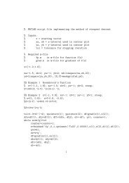

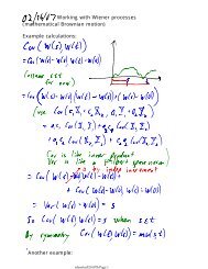

![MATH 1500 Sample Questions Exam 2 1. [3.7] A 10-ft plank is ...](https://img.yumpu.com/43861920/1/190x245/math-1500-sample-questions-exam-2-1-37-a-10-ft-plank-is-.jpg?quality=85)