Some techniques for shading machine renderings of solids

Some techniques for shading machine renderings of solids
by ARTHUR APPEL
IBM Research Center
Yorktown Heights, N. Y.
INTRODUCTION
Some applications of computer graphics require a
vivid illusion of reality. These include the spatial
organization of machine parts, conceptual architectural
design, simulation of mechanisms, and industrial
design. There has been moderate success in the
automatic generation of wire frame, 1 cardboard
model, 2 polyhedra, 3,4 and quadric surface 5 line drawings.
The capability of the machine to generate vivid
sterographic pictures has been demonstrated. 6
There are, however considerable reasons for developing
techniques by which line drawings of solids
can be shaded, especially the enhancement of the
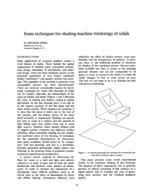
sense of solidity and depth. Figures 1 and 2 illustrate
the value of shading and shadow casting in spatial
description. In the line drawing there is no clue as
to the relative position of the flat plane and the
sheet metal console. When shadows are rendered, it
is clear that the plane is below and to the rear of
the console, and the hollow nature of the sheet
metal assembly is emphasized. Shading can specify
the tone or color of a surface and the amount of
light falling upon that surface from one or more
light sources. Shadows when sharply defined tend
to suggest another viewpoint and improves surface
definition. When controlled, shading can also emphasize
particular parts of the drawing. If techniques
for the automatic determination of chiaroscuro
with good resolution should prove to be competitive
with line drawings, and this is a possibility,
machine generated photographs might replace line
drawings as the principal mode of graphical communication
in engineering and architecture.
A picture strictly rendered in chiaroscuro defines
the scene in a dark and light area pattern,
colored or in tones of grey and no lines are made.
Rembrandt and Reubens were masters of chiaroscuro.
In order to simulate the chiaroscuro of a
photograph many difficult problems need to be
solved such as the effect of illumination by direct
and diffuse lighting, atmospheric diffusion, back
37
reflection, the effect of surface texture, tonal specification,
and the transparency of surfaces. At present,
there is the* additional problem of hardware
for display of the calculated picture. Devices presently
available use lines or points as the principal
pictorial element and are not comparable to oil
paint, or wash, or crayon in the ability to render the
subtle changes in tone or color across an area.
The best we can hope to do is to simulate the halftone
process of printing.
Figure 1—A machine generated line drawing of an electrical console
and an arbitrary plane in space
This paper presents some recent experimental
results in the automatic shading of line drawings.
The purpose of these experiments was to generate
pictures of objects consisting of flat surfaces on a
digital plotter and to evaluate the cost of generating
such pictures and the resultant graphical
quality.

Spring Joint Computer Conference, 1968
Figure 2 —A shaded line drawing of the scene in Figure 1
Previous work
Considerable work has been done in the digitizing
of photographs. 7,8 Especially successful are the
pictures transmitted from spacecraft. 9 The significance
of this work is the demonstration of the quality of
digitally generated pictures.
L. G. Roberts has accomplished the converse of the
problem being discussed in this paper by developing
techniques for the machine perception of solids which
are assemblies of convex poiyhedra modules. 10
His work suggests the possibility that it may be
more useful to analyze the contents of a photograph
and to create a mathematical model of the scene.
This analysis can be used to generate any view of
the scene with greater graphical control.
G. Lasher has written a program which can be
used to generate three dimensional graphs of mathematical
functions which are unique for values of
X and Y. This program, which was used to illustrate
an article in theoretical physics, 11 generates contour
curves of the surface, constant coordinate
curves and renders only those curve segments that
are visible in a perspective projection. A shading
effect occurs in these pictures because the projection
of the surface rulings tend to concentrate as the
surface becomes tangent to the line of sight. This
effect contributes significantly to the vividness of
the renderings.
J. L. Pfaltz and A. Rosenfeld have applied their
notions on encoding plane regions to shading two
dimensional maps. 12 Their notion of skeleton representation
is that a region can be specified by a list
of points on a plane and a radius; all parts of the plane
within the radius of the point are within the region
described. For shading, a set of parallel straight lines
are generated and those portions of the lines which be
within the region are rendered. The angle and spacing
of the set of parallel lines can be varied and other
textures can be generated.
A vivid automatically shaded picture of a polyhedron
was generated by a subroutine written by
B. Archer for an article by A. T. Coie. 13 The shading
is accomplished by varying the spacing of parallel
lines. The spacing of lines on a particular surface
is proportional to the illumination. No attempt was
made to determine the shadow cast by the polyhedron
and the methods described are inadequate for drawing
more than one convex poiyhedra at a time.
Recently, C. Wylie, G. Romney, D. Evans, and A.
Erdahl 13 published an algorithm for generation of
half-tone pictures of objects described by assemblies
of triangular bounded planes. Their results are toned
pictures generated with calculation time competitive
with line drawings. However their scheme sets
the source of illumination at the viewpoint, and since
a point light source cannot see the shadows it casts,
no shadows are rendered.
Previous work in the automatic determination of
chiaroscuro demonstrates how the computer can
improve the level of graphics designers can work with.
The primary limitation has been neglect of shadow
casting from arbitrarily located light sources. Also
no work has been done on the control of the toned
picture to take into account the surface tone or color
of an object. Any system for rendering in chiaroscuro
should solve economically at least these two problems.
It can be seen from previous results that toning an
area by varying the spacing of parallel lines is not
entirely satisfactory. This technique is economic but
has several disadvantages. The lines when widely
spaced do not fuse to form a continuous tone. The
viewer does not then perceive the object but is distracted
by the two dimensional pattern. Depth perception
is reduced. These lines aiso tend to suggest
a surface finish which may not exist. A good standard
for evaluating toning mechanics can be the ben-day
pattern used in printing. This pattern enables a great
range of dark and light with good tonal fusion. The
half-tone process uses many small dots arranged in a
regular array. The size of dots are varied to create a
degree of grayness, small dots where white predominates
are light and as the dots increase in size such that

they eventually blend together the toned region becomes
darker. In order for the dot pattern not to be
distracting, the dot spacing should be at least seventy
dots to the inch. The large dot density required for
toning indicates that calculation schemes for toning
should be as resolution independent as possible. For
an algorithm to be resolution independent it must
enable perfect resolution. It may not be possible for
contemporary hardware to take advantage of such an
algorithm but this should be the goal.
Toning on a digital plotter
A great many experiments were conducted to
evaluate the quality of various toning techniques that
would be applicable to digital plotting. A simulation
technique tested was to shoot random light rays from
the light source at the scene and project a symbol
from the piercing point on the first surface the light
ray pierced. These symbols would concentrate in
regions of high light intensity, and a negative print of
the hard copy could be made which would approximate
a photograph if enough light rays are generated.
Even for about 1000 light rays results were splotchy.
Generating light rays in regular patterns improved the
graphic quality but did not allow economic tonal control.
During these experiments, various symbols were
evaluated for graphic quality and speed of plotter
generation. The plus sign or a small square were to
give best results. Eventually the best technique from
graphic and economic considerations for toning was
found to be plus signs arranged in staggered rows
with shadows outlined. This arrangement is most
easily seen in Figure 2. The size of plus signs were to
be rendered proportional to darkness required.
Ignoring atmospheric diffusion, the intensity of
light incident upon a unit plane area from a point
light source is:
I = S (Cosine L)/D 2
where S is the intensity of the light source, L is the
angle of the normal to the plane and direction of light
at the illuminated area, and D is the distance from the
illuminated point to the light source. For experimental
purposes it was assumed that the light source is so far
from the objects being illuminated that variations in
L and D are insignificant. L need be calculated only
once for each surface. Also since we are interested
in simulating illumination only to the extent that comparative
light and darkness of surfaces are displayed
and also because the range of toning on the digital
plotter is limited, we did not concern ourselves with
the actual intensity of the single light source. The
comparative intensity of illumination of a point on
a plane then is proportional to Cosine L. The apparent
illumination of a flat surface then will be constant
Techniques for Shading Machine Renderings of Solids 3 9
over the surface. The digital plotter does not generate
light as a cathode ray tube but makes a dark mark. The
size of this mark should indicate an absence of light.
So the degree of darkness at a point or the size of
plus sign rendered is
H*=l-Cosine L
For simplicity it can be assumed that if a point is
in shadow the largest allowable mark will be rendered
on that point. For point j then, the size of symbol H,
is the maximum symbol Hs. Hs is proportional to the
dot spacing. During early experiments of the size of
symbols rendered on a point not in shadow was
Hj = 1 — Cosine L
However it was found that results were confusing; it
was difficult to detect the difference between surfaces
in shadow and surfaces almost parallel to the direction
of light. In actual viewing of a solid, surfaces almost
parallel to the direction of light reflect a considerable
amount of light due to the surface roughness, but as
soon as the surface faces away from the light source,
no light can be reflected and the apparent illumination
changes sharply. In order to simulate this effect a
contrast factor, h, usually .8, was introduced. So then
Hj = hHs(l -Cosine L) (la)
if the surface point j is on faces the light source and
Hj = Hs if point j is in shadow. (lb)
We are faced now with essentially at least four programming
problems:
1. Given a viewpoint and a mathematically described
scene what is the point in picture to point
in scene correspondence? This problem is to determine
what visible point, if any, on the objects
being rendered project onto a particular point in
the picture plane.
2. Given one or more light sources what is the intensity
of light falling on a point in the scene?
This problem includes the determination of
which regions are in shadow.
3. Given a light source what are the boundaries of
the shadow cast and how much of this cast
shadow can be seen? If the picture could be
rendered large and/or if symbol density could be
large outlining the shadows could be dispensed
with.
4. How can the tone or color of a surface be specified
and how should this specification affect the
tones rendered?
Economic solutions to the first two problems are
most critical. If an economic point to point correspondence
technique could be found that would permit
dense symbol packing, the problem of casting
shadow outlines could be eliminated. The problem of

40 Spring Joint Computer Conference, 1968
determining how much light falls on a flat surface not
in shadow is trivial, and even for curved surfaces this
is not difficult, but economically determining exactly
what regions of the scene are in shadow is a very difficult
problem.
Figure 3 — An assembly of planes which make up a cardboard model
of a building
Figure 4—Another view of the building
Figure 5 — A higher angle view of the building. 7094 calculation time
for this picture was about 30 minutes.
SHADOW
BOUN0ARY
Point by point shading
-LIGHT SOURCE
Figure 6 —Point by point shading
OBSERVER
LINE OF SIGHT
PNp DOES NOT
CORRESPOND TO
ANY POINT ON
THE OBJECT
Point by point shading techniques yield good
graphic results but at large computational times. These
techniques are docile, require the minimum of storage
and enable easily coded graphical experimentation.
Figures 3, 4, and 5 are examples of point by point
shading. Referring to Figure 6, the technique in generating
these pictures was as follows:
1. Determine the range of coordinates of the projection
of the vertex points.
2. Within this range generate a roster of spots
(Pip) in the picture plane, reproject these spots
one at a time to the eye of the observer and generate
the equation of the line of sight to that spot.
3. Determine the first plane the line of sight to a
particular spot pierces. Locate the piercing point
(Pi) in space. Ignore the spots that do not corre-
apoiiu IU pv/iiiua m iiii^ SvCuv ^i np/ -
4. Determine whether the piercing point is hidden
from the light source by any other surface. If the
point is hidden from the light source (for example
P2) or if the surface the piercing point is on
is being observed from its shadow side, mark on
the roster spot the largest allowable plus sign Hs.
If the point in space is visible to the light source
(for example Px) draw a plus sign with dimension
Hj as determined by Equation 1.
This method is very time consuming, usually requiring
for useful results several thousand times as
much calculation time as a wire frame drawing. About
one half of this time is devoted to determining the
point to point correspondence of the projection and
the scene. In order to minimize calculation time for
point by point shading and maintain resolution, techniques
were developed to determine the outline of cast
shadows. Outlining shadows has the advantage that
all regions of dissimilar tones on the picture plane
are outlined. Even when projected shadows are delicate,
and symbol spacing is large, the shadows are
specified and the discontinuity in tone is emphasized.
The strategy for point by point determination of
shadow boundaries is as follows: (Referring to Figure
7)
TYPICAL
SHADOW
CASTING
LINE
NON-SHADOW
CASTING LINE
rLIGHT SOURCE
-SURFACE UPON WHICH
SHADOW WILL FALL
Figure 7 —Segment by segment outlining of shadows

1. Classify all surface line boundaries into shadow
casting and non-shadow casting. A shadow casting
line is from the viewpoint of an observer
at the light source a contour line. For assemblies
of flat surfaces, a contour line along which all
surfaces associated with this line appear on only
one side of this line.
2. Determine whether the observer is on the shadow
side or lighted side of all surfaces.
3. Subdivide all shadow casting lines, one at a
time, into small segments (Kl, K2), usually .005
units, and determine the midpoint of this segment
(KM).
4. Generate a light ray to the midpoint of the segment
(KM). If any surface lies between KM and
the light source go on to the next segment. Determine
the next surface behind KM that the light
ray to KM pierces within its boundary. If no surface
lies behind KM go on to the next segment.
A point can cast only one shadow. Project Kl,
KM, and K2 onto the surface to obtain K1S,
KMS, and K2S, the shadows of Kl, KM, and
K2. If KMS lies on a surface which is seen from
its shadow side go on to the next segment. This
particular shadow boundary is invisible. Also
a shadow cannot fall within a shadow.
5. Test KMS for visibility. If KMS is hidden from
the observer go on to the next segment.
6. If KMS is visible project the line (K1S-K2S)
onto the picture plane and draw the projection.
As can be expected, determining the outline of
shadows by this described strategy is very time
consuming usually requiring as much time as a point
by point line visibility determination.
Methods of quantitative invisibility
In a previous report, the notion of quantitative
invisibility was discussed as the basis for rapidly determining
the visibility of lines in the line rendering of
polyhedra. 4 P. Loutrell has implemented several tactical
improvements for this application. 15 Quantitative
invisibility is the count of all surfaces, seen from
their spatial side, which hide a line from an observer
at a given point on the line.
The methods of quantitative invisibility are useful
because techniques for detecting changes in quantitative
invisibility along a line are more economical
than measuring the visibility, absolute or quantitative,
at a single point. These techniques are applicable only
to material lines which are lines that have specific end
points and that do not pierce any bounded surface
within its boundary. Objects that are manufactured
contain only material lines. A contour line is a line
along which the line of sight is tangent to the surface
Techniques for Shading Machine Renderings of Solids 41
of the solid. For polyhedra, given a specific viewpoint,
a contour line is a material line which is the intersection
of two surfaces, one of which is invisible.
For a given viewpoint the quantitative invisibility of
a material line can change only when it passes behind
a contour line. Figure 8 illustrates how quantitative
invisibility varies as a line passes behind a solid.
Notice that only surfaces which are viewed from the
spatial side affect the measurement of quantitative
invisibility. In determing line visibility for line drawings
only those segments of the line for which quantitative
invisibility is zero are drawn. For this application
only the quantitative invisibility of vertex points are
stored and changes in quantitative invisibility along
a line are measured and discarded as soon as commands
to the graphic device are generated. The
methods of quantitative invisibility can be applied
to shading a picture if the changes in quantitative
invisibility of a line from the light sources and the
observer are stored and compared.
Figure 8 - Changes in quantitative invisibility. Object A is in front
of and does not touch object B
The method of cutting planes
In descriptive geometry, the intersection of simple
quadric surfaces is determined by passing carefully
chosen planes through the quadric surface to determine
the intersection curve of the quadric surface and
the plane; and from these first and second degree
surface intersections the intersection curve of one or
more quadric surfaces can be deduced. This procedure
is time consuming but does solve a problem difficult
for most mathematicians. This technique of manual
rendering is the inspiration for the method of cutting
planes for shading machine renderings of solids. Point
by point shading techniques are expensive because

42 Spring Joint Computer Conference, 1968
it is difficult with good resolution to correlate the
shading of adjacent spots on the picture plane. With
simple codings, the method of cutting planes enables
such correlation in one direction, with more elaborate
coding the correlation can be in all directions.
The basic concept of the method of cutting planes
is that when the intersections of a plane that passes
through the observation point and assemblies of planes
which can enclose one or more polyhedra are projected
onto the picture plane, these projected intersections
are colinear. In detail, as illustrated in Figure
9, the strategy is:
ICS (INTERSECTION OF CUTTING
i PLANE AND SOLID)
LIGHT SOURCE
TYPICAL
ILLUMINATION
SWEEP PLANE
PICTURE PLANE
ICPONTERSECTION
OF CUTTING PLANE
a PICTURE PLANE)
OBSERVER
TYPICAL CUTTING PLANE
PROJECTIONS OF ICJ.ICK
ONTO PICTURE PLANE.
Figure 9 —The method of cutting planes
1. Generate a cutting plane which passes through
the observation point.
2. This cutting plane will intersect the picture plane
along a specific line (ICP).
3. This cutting plane will cut or pass through the
surfaces of the polyhedra and generate the intersection
ICS which is a string of three or more line
segments. Each of these segments is a material
line (ICJ).
4 All the ICJ of the polyhedral faces and a particular
cutting plane will project colinear onto the
picture plane. This colinear projection is the line
ICP.
These intersections ICJ for a particular cutting
plane can then be measured for changes in quantitative
invisibility by techniques previously reported
4,15 . Those intersections ICJ which
prove to be completely invisible can be quickly
determined and need be analyzed no further. We
have now determined a correspondence between
a line on the picture plane and a series of lines
in the scene to be rendered.
Those lines of intersection ICJ which are on surfaces
which face away from the light source can
be rendered with no further analysis. These
lines are completely in shadow and along their
visible projected length plus signs of the maximum
size (Hs) can be generated.
Lines of intersection ICJ which are on surfaces
which face toward the light source can be analyzed
to determine changes in quantitatives
invisibility from the viewpoint of the light source.
Those projected portions of the lines which are
hidden from the light source are rendered by a
series of plus signs of size Hs. Those portions
which are visible to the light source are rendered
by a series of plus signs whose size is determined
by Equation 1.
Figure 10 —Two views of a machine part where the light source is
moved relative to the object

The resolution of shading by the method of cutting
planes is no longer limited by the spot to spot spacing
on the picture plane but by the spacing of the cutting
planes intersections with the picture plane. For comparable
resolution the calculation time for shading by
cutting planes is slightly less than the square root of
the time for shading by point by point methods.
Figure 11 — Another machine part. 7094 calculation time for this
picture was about 30 seconds
The speed of calculation is very dependent on how
effectively the measurements of quantitative invisibility
of all the lines in the scene are stored and correlated.
This list is the basis for determining visibility
along cutting plane intersections. The first version of
the Fortran IV program used to generate Figures 10
to 14 was experimental and is not as fast as theoretically
expected. Pictures were plotted on an IBM
1627 (Calcomp). A faster version which can take
into account more than one light source is under development
for operation on a 360/67. The larger core,
greater data storage capacity and time sharing capability
of this machine will be utilized. The method of
cutting planes which enable rapid correspondence of
projected points to real points in the scene certainly
includes the illumination of the object by more than
one light source of differing intensities. The size of
Techniques for Shading Machine Renderings of Solids 43
Figure 12 — Assembly of the two previously drawn machine parts.
7094 calculation time: about 50 seconds.
plus signs drawn on a particular spot can be the sum
of the shadow intensity from all the light sources.
HDRAWN = 2 H i ( 2 >
where H is the shadow intensity from a particular
light source.
The more intense the light source, the more intense
the shadow it causes when a point cannot see this
source of light,
I TOTAL = 5)1, (3)
where I is the intensity of the light source
Hsi = VI TOTAL (4)
Where Hsi is the shadow intensity in the absence of
light from light source i.
Hj = Hsi when a point is in shadow
Hi = Hsi(l-CosineL)h (5)
when a point is seen by light source i.
It is also possible to exercise tone control for emphasis
while generating the half-tone picture. A list
of comparative surface tones can be entered which
will describe the basic tone of each surface. For example,
if a scene consists of object A with four sur-

Spring Joint Computer Conference, 1968
faces and object B with six surfaces and object A is
lighter than object B the surface tone list would be
(.5, .5, .5, .5, 1.0, 1.0, 1.0, 1.0, 1.0, 1.0). The size
of the shading symbol can then be determined by
HTik = (Hi X FLIGHT + FTONE) TONEk (6)
where FLIGHT and FTONE are influence factors of
light and surface tone, and TONEk is the relative tone
Figure 13 —Another machine part
Figure 14 —Another view of the machine part shown in the previous
figure.. The light source has been moved relative to the object. Notice
the light passing through the opening in the object
of surface k. FLIGHT and FTONE enable the control
of highlighting. Master copy for the preparation
of color process plates for letterpress printing have
been generated using mathematical models similar to
equation 6= It is obvious that once the basic problems
of determining how light falls on the object are
solved, considerable artistic freedom is possible.
Figure 15 —Assembly of the three machine parts. 7094 calculation
time for this view was about two minutes
ACKNOWLEDGMENTS
The author is grateful to G. Folchi, Dr. G. Lasher,
and Dr. P. Loutrell for some helpful discussions. R.
L. Ennis, J. J. Gordineer, J. A. Mancini, Mr. & Mrs. E.
P. McGilton, W. H. Murray, and G. J. Walsh among
others were helpful with plotter output and other
machine problems. The author is deeply indebted to J.
P. Gilvey and F. L. Graner for their continuing support
and encouragement of this project.
REFERENCES
1 T E JOHNSON
Sketchpad III: A computer program for drawing in three
dimensions.
Proc AFIPS 1963 Spring Joint Computer Conf Vol 23 pp
347-353
2. A APPEL
The visibility problem and machine rendering of solids
IBM Research Report RC 1618 May 20 1966

3 P LOUTREL
Determination of hidden edges in polyhedral figures: convex
case
Technical Report 400-145, Laboratory for Electroscience
Research NYU September 1966
4 A APPEL
The notion of quantitative invisibility and the machine rendering
of solids
Proc ACM 1967 Conference pp 387-393
5 R A WEISS
BE VISION a package of IBM 7090 Fortran programs to draw
orthographic views of combinations of plane and quadric surfaces
J ACM 13 April 1966 11 194-204
6 H R PUCKETT
Computer method for perspective drawing journal of spacecraft
and rockets
Vol I No 1 pp 44-48 1964
7 W S HOLMES H R LELAND G E RICHMOND
Design of a photo interpretation automaton
AFIPS Conf Proceedings 1962 Fall Joint Computer Conference
Vol 22 pp 27-35
8 R W CONN
Digitized photographs for illustrated computer output
AFIPS Conference Proceedings 1967 Spring Joint Computer
Techniques for Shading Machine Renderings of Solids 45
Conference Vol 30 pp 103-106
9 Lunar Orbiter Surveys the Moon Sky and Telescope Vol 32
No 4 October 1966 pp 192-197
10 L G ROBERTS
Machine perception of three-dimensional solids
Technical Report No 315 Lincoln Laboratory MIT May 1963
11 G LASHER
Mixed state oftype-l superconducting films in a perpendicular
magnetic filed
The Physical Review Vol 154 No 2 pp 345-348 Feb 10
1967
12 J L PFALTZ A ROSENFELD
Computer representation of planar regions by their skeletons
CACM Vol 10 No 2 February 1967 pp 119-125
13 A J COLE
Plane and stereographic projections of convex polyhedra from
minimal information
The Computer Journal
14 C WYLIE G ROMNEY D EVANS A ERDAHL
Half-tone perspective drawings by computer
AFIPS Conf proceedings 1967 Fall Joint Computer Conference
Vol 27
15 P LOUTRELL
Phd Thesis NYU September 1967
NYU September 1967