A Guide to Imputing Missing Data with Stata Revision: 1.4

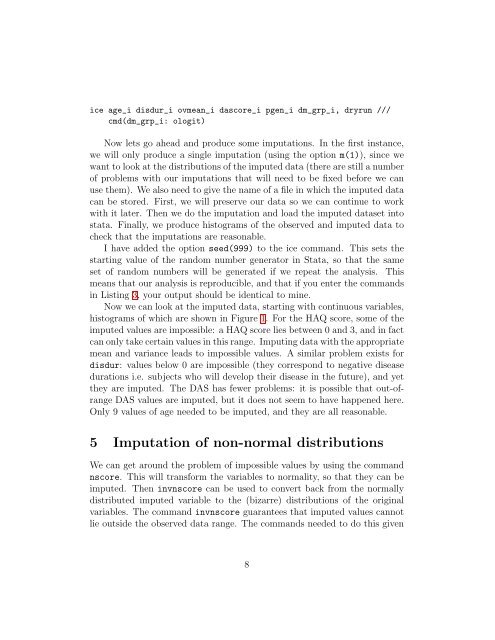
ice age_i disdur_i ovmean_i dascore_i pgen_i dm_grp_i, dryrun ///
cmd(dm_grp_i: ologit)
Now lets go ahead and produce some imputations. In the first instance,
we will only produce a single imputation (using the option m(1)), since we
want to look at the distributions of the imputed data (there are still a number
of problems with our imputations that will need to be fixed before we can
use them). We also need to give the name of a file in which the imputed data
can be stored. First, we will preserve our data so we can continue to work
with it later. Then we do the imputation and load the imputed dataset into
stata. Finally, we produce histograms of the observed and imputed data to
check that the imputations are reasonable.
I have added the option seed(999) to the ice command. This sets the
starting value of the random number generator in Stata, so that the same
set of random numbers will be generated if we repeat the analysis. This
means that our analysis is reproducible, and that if you enter the commands
in Listing 3, your output should be identical to mine.
Now we can look at the imputed data, starting with continuous variables,
histograms of which are shown in Figure 1. For the HAQ score, some of the
imputed values are impossible: a HAQ score lies between 0 and 3, and in fact
can only take certain values in this range. Imputing data with the appropriate
mean and variance leads to impossible values. A similar problem exists for
disdur: values below 0 are impossible (they correspond to negative disease
durations i.e. subjects who will develop their disease in the future), and yet
they are imputed. The DAS has fewer problems: it is possible that out-ofrange
DAS values are imputed, but it does not seem to have happened here.
Only 9 values of age needed to be imputed, and they are all reasonable.
5 Imputation of non-normal distributions
We can get around the problem of impossible values by using the command
nscore. This will transform the variables to normality, so that they can be
imputed. Then invnscore can be used to convert back from the normally
distributed imputed variable to the (bizarre) distributions of the original
variables. The command invnscore guarantees that imputed values cannot
lie outside the observed data range. The commands needed to do this given
8