Introduction to the GRAPE Algorithm - of Michael Goerz
Introduction to the GRAPE Algorithm - of Michael Goerz
Introduction to the GRAPE Algorithm - of Michael Goerz

Create successful ePaper yourself
Turn your PDF publications into a flip-book with our unique Google optimized e-Paper software.
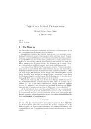
<strong>Introduction</strong> <strong>to</strong> <strong>the</strong> <strong>GRAPE</strong> <strong>Algorithm</strong><br />
<strong>Michael</strong> <strong>Goerz</strong><br />
June 8, 2010<br />
<strong>Michael</strong> <strong>Goerz</strong> <strong>Introduction</strong> <strong>to</strong> <strong>the</strong> <strong>GRAPE</strong> <strong>Algorithm</strong>
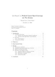
Reference: J. Mag. Res. 172, 296 (2005)<br />
Abstract<br />
Journal <strong>of</strong> Magnetic Resonance 172 (2005) 296–305<br />
Optimal control <strong>of</strong> coupled spin dynamics: design <strong>of</strong> NMR<br />
pulse sequences by gradient ascent algorithms<br />
Navin Khaneja a, *, Timo Reiss b , Cindie Kehlet b , Thomas Schulte-Herbrüggen b ,<br />
Steffen J. Glaser b, *<br />
a Division <strong>of</strong> Applied Sciences, Harvard University, Cambridge, MA 02138, USA<br />
b Department <strong>of</strong> Chemistry, Technische Universität München, 85747 Garching, Germany<br />
Received 27 June 2004; revised 23 Oc<strong>to</strong>ber 2004<br />
Available online 2 December 2005<br />
www.elsevier.com/locate/jmr<br />
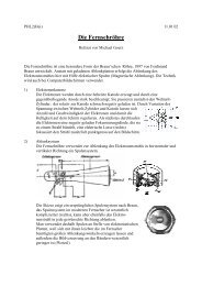
In this paper, we introduce optimal control algorithm for <strong>the</strong> design <strong>of</strong> pulse sequences in NMR spectroscopy. This methodology<br />
is used for designing pulse sequences that maximize <strong>the</strong> coherence transfer between coupled spins in a given specified time, minimize<br />
<strong>the</strong> relaxation effects in a given coherence transfer step or minimize <strong>the</strong> time required <strong>to</strong> produce a given unitary propaga<strong>to</strong>r, as<br />
desired. The application <strong>of</strong> <strong>the</strong>se pulse engineering methods <strong>to</strong> design pulse sequences that are robust <strong>to</strong> experimentally important<br />
parameter variations, such as chemical shift dispersion or radi<strong>of</strong>requency (rf) variations due <strong>to</strong> imperfections such as rf inhomogeneity<br />
is also explained.<br />
<strong>Michael</strong> <strong>Goerz</strong> <strong>Introduction</strong> <strong>to</strong> <strong>the</strong> <strong>GRAPE</strong> <strong>Algorithm</strong>
lse debsenceracterion<br />
<strong>of</strong><br />
5]<br />
The Basic Idea<br />
ð1Þ<br />
re <strong>the</strong><br />
<strong>to</strong> <strong>the</strong><br />
,um(t))<br />
anged<br />
oblem<br />
ds that<br />
a specimumermiasured<br />
ð2Þ<br />
ra<strong>to</strong>rs,<br />
<strong>of</strong> <strong>the</strong><br />
kj is <strong>the</strong> backward propagated target opera<strong>to</strong>r C at <strong>the</strong><br />
same time t = jDt. Let us see how <strong>the</strong> performance U0 changes when we perturb <strong>the</strong> control amplitude uk (j)<br />
at time step j <strong>to</strong> uk(j) +duk(j). From Eq. (4), <strong>the</strong> change<br />
in Uj <strong>to</strong> first order in duk(j) is given by<br />
dU j ¼ iDtdukðjÞHkU j ð8Þ<br />
Acronym<br />
with<br />
Z Dt<br />
HkDt ¼ U jðsÞH kU jð sÞds ð9Þ<br />
0<br />
<strong>GRAPE</strong>: Gradient Ascent Pulse Engineering<br />
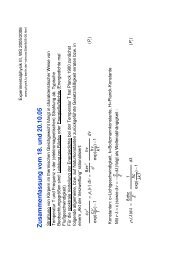
Fig. 1. Schematic representation <strong>of</strong> a control amplitude u k(t),<br />
consisting <strong>of</strong> N steps <strong>of</strong> duration Dt = T/N. During each step j, <strong>the</strong><br />
control amplitude uk(j) is constant. The vertical arrows represent<br />
gradients dU0=dukðjÞ, indicating how each amplitude u k(j) should be<br />
modified in <strong>the</strong> next iteration <strong>to</strong> improve <strong>the</strong> performance function U0.<br />
Pulse Update<br />
Φ0<br />
uk(j) −→ uk(j) + ɛ ∂Φ0<br />
∂uk(j)<br />
original value<br />
uk(j)<br />
at time index j: go in direction <strong>of</strong> gradient<br />
<strong>Michael</strong> <strong>Goerz</strong> <strong>Introduction</strong> <strong>to</strong> <strong>the</strong> <strong>GRAPE</strong> <strong>Algorithm</strong>
Working in Liouville Space<br />
Density Matrix<br />
Liouville-von Neumann Equation<br />
Time Propagation<br />
˙ρ(t) = −i [H, ρ(t)] − = −i<br />
Uj = exp<br />
(<br />
|Ψ〉 −→ ρ = |Ψ〉〈Ψ|<br />
−i∆t<br />
"<br />
H0 +<br />
H0 +<br />
mX<br />
! #<br />
uk(t)Hk , ρ<br />
k=1<br />
mX<br />
!)<br />
uk(j)Hk<br />
k=1<br />
ρ(T ) = UN . . . U1 ρ(0) U †<br />
1 . . . U†<br />
N<br />
= |Ψ(T )〉〈Ψ(T )| with Ψ(T ) = Un . . . U1Ψ(0)<br />
<strong>Michael</strong> <strong>Goerz</strong> <strong>Introduction</strong> <strong>to</strong> <strong>the</strong> <strong>GRAPE</strong> <strong>Algorithm</strong><br />
−
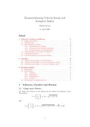
Definition <strong>of</strong> Fidelity<br />
Fidelity in Liouville space is defined in analogy <strong>to</strong> fidelity in Hilbert space: as <strong>the</strong><br />
overlap between <strong>the</strong> propagated state with <strong>the</strong> optimal state.<br />
Fidelity<br />
“<br />
Φ0 = 〈C|ρ(T )〉 ≡ tr C † ”<br />
ρ(T )<br />
C = O |Ψ(0)〉〈Ψ(0)| O †<br />
ρ(T ) = U |Ψ(0)〉〈Ψ(0)| U †<br />
<strong>Michael</strong> <strong>Goerz</strong> <strong>Introduction</strong> <strong>to</strong> <strong>the</strong> <strong>GRAPE</strong> <strong>Algorithm</strong>
Definition <strong>of</strong> Fidelity<br />
Fidelity in Liouville space is defined in analogy <strong>to</strong> fidelity in Hilbert space: as <strong>the</strong><br />
overlap between <strong>the</strong> propagated state with <strong>the</strong> optimal state.<br />
Fidelity<br />
“<br />
Φ0 = 〈C|ρ(T )〉 ≡ tr C † ”<br />
ρ(T )<br />
C = O |Ψ(0)〉〈Ψ(0)| O †<br />
Equivalence <strong>to</strong> “normal” fidelity<br />
“<br />
tr C † ”<br />
ρ(T )<br />
ρ(T ) = U |Ψ(0)〉〈Ψ(0)| U †<br />
= X D ˛ ˛ E D ˛<br />
˛ ˛<br />
˛<br />
n ˛O ˛ Ψ(0) Ψ(0) ˛O<br />
n<br />
† ˛ E D ˛<br />
˛<br />
˛<br />
U˛<br />
Ψ(0) Ψ(0) ˛U †˛ E<br />
˛ n<br />
D ˛<br />
= Ψ(0) ˛U † X˛ E D ˛ ˛ E D ˛<br />
˛˛ ˛ ˛<br />
˛<br />
n n ˛ O ˛ Ψ(0) Ψ(0) ˛O † ˛ E<br />
˛<br />
U˛<br />
Ψ(0)<br />
D ˛<br />
= Ψ(0) ˛U † ˛ E D ˛<br />
˛<br />
˛<br />
O˛<br />
Ψ(0) Ψ(0) ˛O † ˛ E<br />
˛<br />
U˛<br />
Ψ(0)<br />
˛D<br />
˛<br />
˛ ˛<br />
= ˛ Ψ(0) ˛O † ˛ E˛<br />
˛ ˛˛ 2<br />
U˛<br />
Ψ(0)<br />
<strong>Michael</strong> <strong>Goerz</strong> <strong>Introduction</strong> <strong>to</strong> <strong>the</strong> <strong>GRAPE</strong> <strong>Algorithm</strong>
Fidelity through Backward- and Forward-Propagation<br />
A trace is invariant under cyclic permutation <strong>of</strong> its fac<strong>to</strong>rs!<br />
Fidelity at T<br />
D<br />
Φ0 = 〈C|ρ(T )〉 = C|UN . . . U1ρ(0)U †<br />
E<br />
1 . . . U†<br />
N<br />
D<br />
= U †<br />
j+1 . . . U†<br />
NCUN . . . Uj+1|Uj . . . U1ρ(0)U †<br />
E<br />
1 . . . U†<br />
j<br />
Propagated States → Fidelity at tj<br />
λj ≡ U †<br />
j+1 . . . U†<br />
NCUN . . . Uj+1 bw. propagated optimal state<br />
ρj ≡ Uj . . . U1ρ(0)U †<br />
1 . . . U†<br />
j fw. propagated initial state<br />
Φ0 = 〈C|ρ(T )〉 = ˙ ¸<br />
λj |ρj<br />
Note: all propagations with guess pulse!<br />
<strong>Michael</strong> <strong>Goerz</strong> <strong>Introduction</strong> <strong>to</strong> <strong>the</strong> <strong>GRAPE</strong> <strong>Algorithm</strong>
Calculation <strong>of</strong> Pulse Update<br />
Pulse Update<br />
Two steps:<br />
uk(j) −→ uk(j) + ɛ ∂Φ0<br />
∂uk(j)<br />
For a variation δuk(j), calculate δUj<br />
Use δUj <strong>to</strong> calculate ∂Φ0<br />
∂u k (j)<br />
Calculations are not completely trivial.<br />
Solution:<br />
Gradient<br />
We need <strong>to</strong> calculate ∂Φ0<br />
∂uk(j)<br />
∂Φ0<br />
∂uk(j) = − ˙ ¸<br />
λj |i∆t[Hk, ρj ]−<br />
<strong>Michael</strong> <strong>Goerz</strong> <strong>Introduction</strong> <strong>to</strong> <strong>the</strong> <strong>GRAPE</strong> <strong>Algorithm</strong>
Grape <strong>Algorithm</strong><br />
Pulse Update<br />
uk(j) −→ uk(j) + ɛ ∂Φ0<br />
∂uk(j) ;<br />
Guess initial controls uk(j)<br />
Update pulse according <strong>to</strong> gradient:<br />
∂Φ0<br />
∂uk(j) = − ˙ ¸<br />
λj |i∆t[Hk, ρj ]−<br />
Forward propagation <strong>of</strong> ρ(0): calculate and s<strong>to</strong>re all ρj = Uj . . . U1ρ(0)U †<br />
1<br />
for j ∈ [1, N]<br />
. . . U†<br />
j<br />
Backward propagation <strong>of</strong> C: calculate and s<strong>to</strong>re all λj = U †<br />
j+1 . . . U†<br />
NCUN . . . Uj+1<br />
for j ∈ [1, N]<br />
Evaluate ∂Φ0 and update <strong>the</strong> m × N control amplitudes uk(j)<br />
∂uk (j)<br />
Done if fidelity converges<br />
<strong>Michael</strong> <strong>Goerz</strong> <strong>Introduction</strong> <strong>to</strong> <strong>the</strong> <strong>GRAPE</strong> <strong>Algorithm</strong>
Variations<br />
Non-Hermitian Opera<strong>to</strong>rs<br />
Φ1 = ℜ[Φ0];<br />
Φ2 = |Φ0| 2 ;<br />
Unitary Transformations<br />
Φ3 = ℜ 〈UF |U(T )〉 = ℜ<br />
D<br />
∂Φ1<br />
= − λ<br />
∂uk(j) x j |i∆t[Hk, ρ x E D<br />
j − λ y<br />
j |i∆t[Hk, ρ y<br />
E<br />
j<br />
∂Φ2<br />
∂uk(j) = −2ℜ ˘˙ ¸ ˙ y<br />
λj |i∆t[Hk, ρj ρN |C¸¯<br />
D<br />
U †<br />
j+1 . . . U†<br />
NUF E<br />
|Uj . . . U1 = ℜ ˙ ¸<br />
Pj |Xj<br />
∂Φ3<br />
∂uk(j) = −ℜ ˙ ¸<br />
Pj |i∆tHkXj<br />
Φ4 = |〈UF |U(T )〉| 2 = ˙ Pj |Xj<br />
¸ ˙ ¸<br />
Xj |Pj<br />
∂Φ4<br />
∂uk(j) = −2ℜ ˘˙ ¸ ˙ ¸¯<br />
Pj |i∆tHkXj Xj |Pj<br />
Also works with Lindbladt-Opera<strong>to</strong>rs. Additional energy constraints are possible.<br />
<strong>Michael</strong> <strong>Goerz</strong> <strong>Introduction</strong> <strong>to</strong> <strong>the</strong> <strong>GRAPE</strong> <strong>Algorithm</strong>
5]<br />
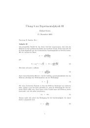
Comparison with with OCT<br />
ð1Þ<br />
re <strong>the</strong><br />
<strong>to</strong> <strong>the</strong><br />
,um(t))<br />
anged<br />
oblem<br />
ds that<br />
a specimumermiasured<br />
ð2Þ<br />
ra<strong>to</strong>rs,<br />
<strong>of</strong> <strong>the</strong><br />
j k k j<br />
Z Dt<br />
HkDt ¼ U jðsÞH kU jð sÞds ð9Þ<br />
0<br />
Fig. 1. Schematic representation <strong>of</strong> a control amplitude u k(t),<br />
consisting <strong>of</strong> N steps <strong>of</strong> duration Dt = T/N. During each step j, <strong>the</strong><br />
control amplitude uk(j) is constant. The vertical arrows represent<br />
gradients dU0=dukðjÞ, indicating how each amplitude u k(j) should be<br />
modified in <strong>the</strong> next iteration <strong>to</strong> improve <strong>the</strong> performance function U0.<br />
Ψin<br />
ɛ (1)<br />
ɛ (0)<br />
∆u(j) ∼ ˙ Ψbw (tj ) |µ| Ψfw (tj ) ¸<br />
<strong>GRAPE</strong> also needs forward- and backward-propagation, but only with old pulse.<br />
Propagated states also need <strong>to</strong> be s<strong>to</strong>red.<br />
Pulse update at point j in <strong>the</strong> current iteration does not depend on o<strong>the</strong>r<br />
updated pulse values (non-sequential update)<br />
All updates in <strong>GRAPE</strong> can in principle be calculated in parallel.<br />
Convergence tends <strong>to</strong> be pretty lousy (so I’m <strong>to</strong>ld)<br />
What about <strong>the</strong> choice <strong>of</strong> ɛ?<br />
<strong>Michael</strong> <strong>Goerz</strong> <strong>Introduction</strong> <strong>to</strong> <strong>the</strong> <strong>GRAPE</strong> <strong>Algorithm</strong><br />
tj<br />
Ψtgt
Thank You!<br />
<strong>Michael</strong> <strong>Goerz</strong> <strong>Introduction</strong> <strong>to</strong> <strong>the</strong> <strong>GRAPE</strong> <strong>Algorithm</strong>