Exploring the Methods of Differential Calculus through the ...

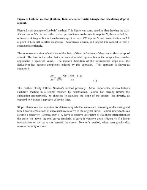
Figure 2. Leibniz’ method (Leibniz, 1684) of characteristic triangles for calculating slope at
a point.
Figure 2 is an example of Leibniz’ method. This figure was constructed by first drawing the axis
AX and curve VV. A line is then drawn perpendicular to the axis from point V, this is called the
ordinate v. A tangent line is then drawn tangent to curve VV at point V and connected to axis AX
at point B. Line XB is called an absissa. The ordinate, absissa, and tangent line connect to form a
characteristic triangle.
The more modern view of calculus unifies both of these definitions of slope under the concept of
a limit. The limit is the value that a dependent variable approaches as the independent variable
approaches a specified value. The modern definition of the infinitesimal slope (i.e., the
derivative) has become completely colored by this approach. This approach is shown as
equation 1:
This method clearly follows Newton’s method precisely. More importantly, it also follows
Leibniz’s method in a simple manner; by construction, Leibniz had already limited the
calculation geometrically by choosing to calculate the slope of the tangent line directly, as
opposed to Newton’s approach of secant lines.
Slope calculations are important for determining whether curves are increasing or decreasing and
how linear interpolations of curves behave relative to the original curve. Leibniz refers to this as
a curve’s concavity (Leibniz, 1684). A curve is concave up (Figure 3) if a linear interpolation of
the curve sits above the real curve; similarly, a curve is concave down (Figure 4) if a linear
interpolation of the curve sits beneath the curve. Newton’s method, when seen graphically,
makes concavity obvious.
(1)