unit 1 differential calculus - IGNOU

UNIT 1 DIFFERENTIAL CALCULUS 

Structure 

1.1 Introduction 

Objectives 

1.2 Real Number System 

1.3 Functions 

1.3.1 Definition and Examples 

1.3.2 Inverse Functions 

1.3.3 Graphs of Inverse Functions 

1.3.4 New Functions from Old 

1.3.5 Operations on Functions 

1.3.6 Composition of Functions 

1.3.7 Types of Functions 

1.4 Limits 

1.5 Continuity 

1.6 Derivative 

1.6.1 Derivative of a Function 

1.6.2 Algebra of Derivatives 

1.6.3 Derivative of a Composite Function (Chain Rule) 

1.6.4 Second Order Derivatives 

1.6.5 Implicit Differentiation 

1.6.6 Derivatives of Some Elementary Functions 

1.6.7 Derivatives of a Function Represented Parametrically 

1.6.8 Logarithmetic Differentiation 

1.6.9 Differentiation by Substitution 

1.7 Summary 

1.8 Answers to SAQs 

1.1 INTRODUCTION 

Calculus was related to meet the pressing mathematical needs of the 17 th century 

science and is still the fundamental mathematics for solving problems in Science 

and Technology. In this unit, we will introduce the concept of functions and 

discuss different types of functions, algebra of functions and their limit and 

continuity. We will also introduce the concept of derivative as the instantaneous 

rate of change. We shall discuss methods of differentiation. 

Objectives 

After studying this unit, you should be able to 

• recall the basic properties of real numbers, 

• define a function and examine whether a given function is oneone/onto, 

• identify whether a given function has an inverse or not, 

• determine weather a given function is even or odd, 

Differential Calculus 

5

Mathematics-II 

6 

• evaluate the limit of a function at a point, 

• identify points of continuity and discontinuity of a function, and 

• obtain the derivative of a function at a point. 

1.2 REAL NUMBER SYSTEM 

The set of all real numbers is denoted by R. The real number system is the 

foundation on which a large part of mathematics including calculus rests. You are 

familiar with the operations of addition, subtraction, multiplication and division 

of real numbers and with inequalities. We shall recall some of their properties : 

P1 - R is closed under addition. 

P2 - Addition is associative and commutative. 

P3 - R is closed under multiplication. 

P4 - Multiplication is commutative and associative. 

P5 - Multiplication is distributive over addition. 

P6 - For any two real numbers a and b, either a > b or a 

You are also familiar with the following subsets of R. 

(i) N, the set of natural numbers. 

(ii) Z, the set of integers. 

(iii) Q, the set of rational numbers. 

Definition 1 

If x is a real number, its absolute value, denoted by | x | is defined as 

For example 

| x | = x if x ≥ 0 

| 5 | = 5 

= − x if x < 0 

| − 5 | = 5 

The following theorem (without proof) gives some of the important properties 

of | x |. 

Theorem 1 

If x and y are real numbers, then 

(i) | x | = max {− x, x} 

(ii) | x | = | − x | 

(iii) | x | 2 = x 2 = | − x | 2 

(iv) | x + y | ≤ | x | + | y | 

(v) | x − y | ≥ | | x | − | y | |

Definition 2 

Let S be a non-empty subset of R. An element u ∈ R is said to be upper 

bound of S if u ≥ x for all x ∈ S. If S has an upper bound, we say S is 

bounded above. On similar lines we can define a lower bound for a 

non-empty set S to be a real number v such that v ≤ x for all x ∈ S and we 

say that the set S is bounded below. 

1.2.1 Intervals on the Real Line 

Before we define an interval, let us see what is meant by a number line. The real 

numbers in set R can be put into one-to-one correspondence with the points on a 

straight line L. In other words, we shall associate a unique point on L to each real 

number and vice-versa. 

Consider a straight line L (Figure 1.1(a)). Mark a point O on it. The point O 

divides the straight line into two parts. We shall use the part of the left of O for 

representing negative real numbers and the part of the right of O for representing 

positive real numbers. We choose a point A on L which is to the right of O. we 

shall represent the number 0 by O and 1 by A. OA can now serve as a unit. To 

each positive real number, x we can associate exactly one point P lying to the 

right of O on L, so that OP = x units (= x). A negative real number y will be 

represented by a point Q lying to the left of O on the straight line L so that 

OQ = y units (= − y, since y is negative). We thus find that to each real number 

we can associate a point on the line. Also, each point S on the line represents a 

unique real number z, such that z = OS. Further, z is positive if S is to the right of 

O, and is negative if S is to the left of O. 

This representation of real numbers by points on a straight line is often very 

useful. Because of this one-to-one correspondence between real numbers and the 

points of a straight line, we often call a real number “a point of R”. Similarly, L is 

called a “number line”. Note that the absolute value or the modulus of any 

number x is nothing but its distance from the point O on the number line. In the 

same way, x – y denotes the distance between the two numbers x and y (Figure 

1.1(b)). 

− 2 

− 1 

0 

1 2 

Q O A P 

x | x – y | y 

y | x – y | x 

y > x 

y < x 

(a) (b) Distance between x and y is | x – y | 

Figure 1.1 

Now let us consider the set of real numbers which lie between two given real 

numbers a and b. Actually, there will be four different sets satisfying this loose 

condition. These are : 

(i) (a, b) = {x | a < x < b} a b 

(ii) [a, b] = {x | a ≤ x ≤ b} a b 

(iii) (a, b] = {x | a < x ≤ b} a b 

(iv) [a, b) = {x | a ≤ x < b} a b 

Figure 1.1 (c) 


7


8 

The representation of each of these sets is given alongside (Figure 1.1(c)). Each 

of these sets is called an interval, and a and b are called the end points of the 

interval. The interval (a, b), in which the end points are not included, is called an 

open interval. Note that in this case we have drawn a hollow circle around a and 

b to indicate that they are not included in the graph. The set [a, b] contains both 

its end points is called a closed interval. In the representation of this closed 

interval, we have put thick black dots at a and b to indicate that they are included 

in the set. 

The sets (a, b] and [a, b) are called half-open (or half-closed) intervals or 

semi-open (or semi-closed) intervals, as they contain only one end point. This 

fact is also indicated in their geometrical representation. 

Each of these intervals is bounded above by b and bounded below by a. 

Can we represent the set 

I = {x : | x – a | < δ} 

on the number line? Yes, we can. We know that x – a can be thought of as the 

distance between x and a. This means I is set of all numbers x, whose distance 

from a is less than δ. Thus, I is the open interval (a − δ, a + δ). Similarly, 

I1 = {x : | x – a | ≤ δ} 

is the closed interval [a – δ, a + δ]. Sometimes, we also come across sets like 

I2 = {x : | 0 < | x – a | < δ} 

This means if x ∈ I2, then the distance between x and a is less than δ, but is not 

zero. We can also say that the distance between x and a is less than, δ, but x ≠ a. 

Thus, 

I2 = (a – δ, a + δ) – {a} = (a – δ, a) ∪ (a, a + δ) 

Apart from the four types of intervals listed above, there area a few more types. 

These are : 

(a, ∞) = {x | a < x} (open right ray) 

[a, ∞) = {x | a ≤ x} (closed right ray) 

(− ∞, b) = {x | x < b} (open left ray) 

(− ∞, b] = {x | x ≤ b} (closed left ray) 

(− ∞, ∞) = R (open interval) 

As you can see easily, none of these sets is bounded. For instance, (a, ∞) is 

bounded below, but is not bounded above, (− ∞, b) is bounded above, but is not 

bounded below. Note that ∞ does not denote a real number; it merely indicates 

that an interval extends without limit. 

We note further that if S is any interval (bounded and unbounded) and if c and d 

are two elements of S then all numbers lying between c and d are also elements 

of S. 

SAQ 1 

(a) Prove the following using results of Theorem. 

(i) x = 0, iff | x | = 0

1 1 

(ii) = , if x ≠ 0 

x | x| 

(iii) | x − y | ≤ | x | + | y | 

(b) State whether the following are true or false. 

(i) 0 ∈ [1, ∞] True/False 

(ii) − 1 ∈ (− ∞, 2) True/False 

(iii) 1 ∈ [1, 2] True/False 

(iv) 5 ∈ (5, ∞) True/False 

1.3 FUNCTIONS 

Now let us move over to functions. Here we shall present some basic facts about 

functions which will help you refresh your knowledge. We shall look at various 

examples of functions and shall also define inverse functions. Let us start with the 

definition. 

1.3.1 Definition and Examples 

Definition 3 

If X and Y are two non-empty sets, a function f from X to Y is a rule or a 

correspondence which connects every member of X to a unique member 

of Y. We write f : X → Y (reads as “f is a function from X to Y” or “f is a 

function of X into Y”). X is called the domain and Y is called the co-domain 

of f. We shall denote by f (x) that unique element of Y, which corresponds 

to x ∈ X. 

The following examples will help you in understanding this definition better. 

Example 1.1 

Consider f : N → R defined by f (x) = − x. Is “f ” a function? 

Solution 

“f ” is a function since the rule f (x) = − x associates a unique member (− x) 

of R to every member x of N. The domain here is N and the co-domain is R. 

Example 1.2 

x 

Consider f : N → Z, defined by the rule f ( x) 

= . Is “f ” a function? 

2 

Solution 

“f ” is not a function from N to Z as odd natural numbers like 1, 3, 5 . . . 

from N cannot be associated with any member of Z. 

Example 1.3 


9


10 

Consider f : N → N, under the rule f (x) = a prime factor of x. Is “f ” a 

function? 

Solution 

Here, since 6 = 2 × 3, f (6) has two values : f (6) = 2 and f (6) = 3. This rule 

does not associate a unique member in the co-domain with a member in the 

domain and, hence, f, as defined, is not a function of N into N. 

Thus, you see, to describe a function completely we have to specify the following 

three things : 

(i) the domain, 

(ii) the co-domain, and 

(iii) the rule which assigns to each element x in the domain, a single fully 

determined element in the co-domain. 

Given a function f : X → Y, f (x) ∈ Y is called the image of x ∈ X under f or the 

f-image of x. The set of f-images of all number of X, i.e. {f (x) : x ∈ X} is called 

the range of f and is denoted by f (X). It is easy to see that f (X) ⊂ Y. 

Remark 

(i) Throughout this unit we shall consider functions whose domain and 

co-domain are both subsets of R. Such functions are often called real 

functions or real value functions. 

(ii) The variable x used in describing a function is often called a dummy 

variable because it can be replaced by any other letter. Thus, for 

example, the rule f (x) = − x, x ∈ N can as well be written in the form 

f (t) = − t, t ∈ N, or as f (u) = − u, u ∈ N. The variable x (or t or u) is 

also called an independent variable and f (x), which is dependent on 

this independent variable, is called a dependent variable. 

Graph of Function 

A convenient and useful method for studying a function is to study it 

through its graph. To draw the graph of function f : X → Y, we choose a 

system of co-ordinate axes in the plane. For each x ∈ X, the ordered pair 

(x, f (x)) determines a point in the plane (Figure 1.2). The set of all the 

points obtained by considering all possible values of x, that is, 

(x, f (x)) : x ∈ X) is the graph of f. 

0 

y 

(x, f ( x)) 

x 

f (x) 

Figure 1.2 

x

The role that the graph of a function plays in the study of the function will 

become clear as we proceed further. In the meantime let us consider some 

more examples of functions and their graphs. 

A Constant Function 

A simple example of a function is a constant function. A constant 

function sends all the elements of the domain to just one element of 

the co-domain. 

For example, let f : R → R be defined by f (x) = 1. 

Alternatively, we may write 

f : x → 1 for all x ∈ R 

The graph of f is as shown in Figure 1.3. 

1 

0 

y 

f (x) = 1 

Figure 1.3 

It is the line y = 1. 

In general, the graph of a constant function y : x → c is a straight line 

which is parallel to the x-axis at a distance of c units from it. 

The Identity Function 

Another simple but important example of a function is a function 

which sends every element of the domain to itself. 

Let X by any non-empty set, and f be the function of X defined by 

setting f (x) = x, for all x ∈ X. 

This function is known as the identity function on X and is denoted 

by IX. 

The graph of IR, the identity function of R, is shown in Figure 1.4. It is 

the line y = x. 

0 

y 

Figure 1.4 

y = x 

x 

x 


11


12 

Absolute Value Function 

Another interesting function is the absolute value function (or 

modulus function) which can be defined by using the concept of the 

absolute value of a real number as 

⎧ x, 

if x ≥ 0 

f ( x) 

= | x| 

= ⎨ 

⎩− 

x, 

if x < 0 

The graph of this function is shown in Figure 1.5. It consists of two 

3π 

rays, both starting at the origin and making angles and 

4 4 

π 

respectively, with the positive direction of the x-axis. 

The Exponential Function 

θ1 

y 

0 

Figure 1.5 

If a is a positive real number other than 1, we define a function 

f : R → R by f (x) = a x where a > 0, a ≠ 1. 

θ 2 

This function is known as the general exponential function. A special 

case of this function, where a = e, is often found useful. Figure 1.6 

shows the graph of the function f : R → R such that f (x) = e x . This 

function is called the natural exponential function. Its range is the set 

R + of positive numbers. 

− 2 

− 1 

y 

3 

2 

1 

1 

(1, e) 

y = e x 

x 

2 3 

Figure 1.6 

The Natural Logarithmic Function 

This function f : R + → R is defined on the set R + of all real numbers 

f : R + → R such that f (x) = ln (x). The range of this function is R. Its 

graph is shown in Figure 1.7. 

y 

(e, 1) 

y = ln (x) 

x

The Greatest Integer Function 

Figure 1.7 

Take a real number x. Either it is an integer, say n (so that x = n), or it 

is not integer. If it is not an integer, we can find an integer n, such that 

n < x < n + 1. Therefore, for each real number x we can find an 

integer n, such that n < x < n + 1. Further, for a given real number x, 

we can find only one such integer n. We say that n is the greatest 

integer not exceeding x and denote it by [x]. For example, [3] = 3 and 

[3.5] = 3, [− 3.5] = − 4. 

Other Functions 

The following are some important classes of functions. 

Polynomial Functions f (x) = a0 x n + a1 x n − 1 + . . . + an where a0, a1, . . . , an are 

given real numbers (constants) and n is a positive integer. 

We say n is the degree of the polynomial 

f (x) and assume a0 ≠ 0. 

Rational Functions 

g ( x) 

f ( x) 

= , where g (x) and k (x) are polynomial 

k ( x) 

Trigonometrical or 

Circular Functions 

Hyperbolic Functions 

We shall study these in detail in this unit. 

1.3.2 Inverse Functions 

functions of degree n and m respectively. This is defined 

for all real x for which k (x) ≠ 0. 

f (x) = sin x, f (x) = cos x, f (x) = tan x, 

f (x) = cot x, f (x) sec x, and f (x) = cosec x. 

x − x 

( e + e ) 

f ( x) 

= cosh x = , 

2 

x − x 

( e − e ) 

f ( x) 

= sinh x = . 

2 

In this sub-section we shall see what is meant by the inverse of a function. But 

before talking about the inverse, let us look at some special categories of 

functions. These special types of functions will then lead us to the definition of 

inverse of a function. 

One-one and Onto Functions 

Consider the function h : x → x 2 , defined on the set R. Here 

h (2) = h (− 2) = 4; i.e. 2 and – 2 are distinct members of the domain R, but 

their h-images are the same (Can you find some more members whose 

h-images are equal?). In general, this may be expressed by saying : find x, y 

such that x ≠ y but h (x) = h (y). 

Now consider another function g : x → 2x + 3. Here you will be able to see 

that if x1 and x2 are two distinct real numbers, then g (x1) and g (x2) are also 

distinct. 


13


14 

For, 

x ≠ x ⇒ x ≠ 2x 

⇒ 2x 

+ 3 ≠ 2x 

+ 3 ⇒ g( 

x ) ≠ g( 

x ) . 

1 

2 

2 1 2 1 

2 

1 2 

We have considered two functions here. While one of them, namely g, 

sends distinct members of the domain to distinct members of the 

co-domain, the other, namely h, does not always do so. We give a special 

name to functions like g above. 

Definition 4 

A function f : X → Y is said to be a one-one function (a 1–1 function or an 

injective function) if images of distinct members of X are distinct members 

of Y. 

Thus, the function g above is one-one, whereas h is not one-one. 

Remark 

The condition that the images of distinct members of X are distinct 

members of Y in the above definition, can be replaced by either of the 

following equivalent conditions : 

(i) For every pair of members x, y of X, x ≠ y ⇒ f (x) ≠ f (y). 

(ii) For every pair of members x, y of X, f (x) = f (y) ⇒ x = y. 

We have observed earlier that for a function f : X → Y, f (X) ⊆ Y. 

This opens two possibilities : 

(i) f (X) = Y, or 

(ii) f (X) ⊂ Y, that is f (X) is a proper subset of Y. 

The function h : x → x 2 , for all x ∈ R falls in the second category. Since the 

square of any real number is always non-negative, h (R) = R + ∪ (0) which is 

the set of non-negative real numbers. Thus h (R) ⊂ R. 

On the other hand, the function g : x → 2x + 3 belongs to the first category. 

⎛ 1 ⎞ 3 

Given any y ∈ R (co-domain), if we take x = ⎜ ⎟ y − , we find that 

⎝ 2 ⎠ 2 

g (x) = y. This shows that every member of the co-domain is a g-image of 

some member of the domain and, thus, is in the range g. From this, we get 

that g (R) = R. The following definition characterises this property of the 

function. 

Definition 5 

A function f : X → Y is said to be an onto function (or a surjective function) 

if every member of Y is the image of some members of X. 

Thus h is not an onto function, whereas g is an onto function. Functions 

which are both one-one and onto (or bijective) are of special importance in 

mathematics. Let us see what makes them special. 

Consider a function f : X → Y which is both one-one and onto. Since f is an 

onto function, each y ∈ Y is the image of some x ∈ X. Also, since f is 

one-one, y cannot be the image of two distinct members of X. Thus, we find 

that to each y ∈ Y there corresponds a unique x ∈ X such that f (x) = y. 

Consequently, f sets up one-to-one correspondence between the members of 

X and Y. It is the one-to-one correspondence between members of X and Y 

which makes a one-one and onto function so special, as we shall soon see.

Consider the function f : N → E defined by f (x) = 2x, where E is the set of 

even natural numbers. We can see that f is one-one as well as onto. In fact, 

y ⎛ y ⎞ 

to each y ∈ E there exists ∈ N such that f ⎜ ⎟ = y . The correspondence 

2 

⎝ 2 ⎠ 

y 

y 

y → defines a function, say g, from E to N such that g ( y) 

= . 

2 

2 

The function g so defined is called as inverse of f. Since, to each y ∈ E 

there corresponds a unique x ∈ N such that f (x) = y only one such function 

g can be defined corresponding to a given function f. For this reason, g is 

called the inverse of f. 

As you will notice, the function g is also one-one and onto and therefore it 

will also have an inverse. You must have already guessed that the inverse of 

g is the function f. 

From this discussion we have the following : 

If f is one-one and onto function from X to Y, then there exists a unique 

function g : Y → X such that for each y ∈ Y, g (y) = x ⇔ y = f (x). The 

function g so defined is called the inverse of f. Further, if g is the inverse of 

f, then f is the inverse of g, and the two functions f and g are said to be the 

inverse of each other. The inverse of a function f is usually denoted by f – 1 . 

To find the inverse of a given function f, we proceed as follows : 

Solve the equation f (x) = y for x. The resulting expression for x (in terms 

of y) defines the inverse function. 

Thus, if ( ) = + 2, 

5 

x 

f x 

x 

we solve + 2 = y for x 

5 

5 

This gives us x = ( 5( 

y − 2)) 

. 

5 

Hence f – 1 1 

−1 

is the function defined by f ( y) 

= ( 5( 

y − 2)) 

5 . 

1 

5 

1.3.3 Graphs of Inverse Functions 

There is an interesting relation between the graphs of a pair of inverse functions 

because of which, if the graph of one of them is known, the graph of the other can 

be obtained easily. 

Let f : X → Y be a one-one and onto function, and let g : Y → X be the inverse of 

f. A point (p, q) lies on the graph of f ⇔ q = f (p) ⇔ p = g (q) (q, p) lies on the 

graph of g. Now, the point (p, q) and (q, p) are reflections of each other with 

respect to (w. r. t.) the line y = x. Therefore, we can say that the graphs of f and g 

are reflections of each other w. r. t. the line y = x. 

Therefore, it follows that, if the graph of one of the functions f and g is given, that 

of the other can be obtained by reflecting it w. r. t. the line y = x. As an 

illustration, the graphs of the functions x 3 and y = x 1/3 are given in Figure 1.8. 

y 

0 

x 


15


16 

Figure 1.8 

Do you agree that these two functions are inverses of each other? If the sheet of 

paper on which the graph have been drawn is folded along the line y = x, the two 

graphs will exactly coincide. 

If a given function is not one-one on its domain, we can choose a subset of the 

domain on which it is one-one and then define its inverse function. For example, 

consider the function f : x → sin x. 

Since we know that sin (x + 2π) = sin x, obviously this function is not one-one 

⎡ π π⎤ 

on R. But if we restrict it to the intervals ⎢− 

, ⎥ we find that it is one-one. 

⎣ 2 2 ⎦ 

Thus, if 

Then we can define 

⎡ π π⎤ 

f (x) = sin (x), for all x ∈ ⎢− 

, . 

2 2 

⎥ 

⎣ ⎦ 

−1 

−1 

f ( x) 

= sin ( x) 

= y, 

if sin y = x. 

Similarly, we can define cos – 1 and tan – 1 functions as inverse of cosine and 

⎡ π π⎤ 

tangent functions if we restrict the domains to [0, π ] and ⎢− 

, ⎥ respectively. 

⎣ 2 2 ⎦ 

SAQ 2 

(a) Compare the graphs of ln x and e x given in Figures 1.6 and 1.7 and 

verify that they are inverses of each other. 

(b) Which of the following functions are one-one? 

(i) f : R → R defined by f (x) = | x |. 

(ii) f : R → R defined by f (x) = 3x − 1. 

(iii) f : R → R defined by f (x) = x. 

(iv) f : R → R defined by f (x) = 1. 

(c) Which of the following functions are onto? 

(i) f : R → R defined by f (x) = 3x + 7. 

(ii) f : R + → R defined by f (x) = x .

(iii) f : R → R defined by f (x) = x 2 + 1. 

1 

(iv) f : X → R defined by f (x) = where X stands for the set of 

x 

non-zero real numbers. 

x + 1 

(d) Show that the function f : X → X such that f ( x) 

= where X is 

x − 1 

the set of all real number except 1, is one-one and onto. Find its 

inverse. 

(e) Give one example of each of the following : 

(i) a one-one function which is not onto? 

(ii) onto function which is not one-one? 

(iii) a function which is neither one-one nor onto? 

1.3.4 New Functions from Old 

In this sub-section, we shall see how we can construct new functions from some 

given functions. This can be done by operating upon the given functions in a 

variety of ways. We give a few such ways here. 

1.3.5 Operations on Functions 

Scalar Multiple of a Function 

Consider the function f : x → 3x 2 + 1, for all x ∈ R. The function 

g : x → 2 (3x 2 + 1) for all x ∈ R is such that g (x) = 2f (x), for all x ∈ R. We 

say that g = 2f and that g is a scalar multiple of f by 2. In the above 

example, there is nothing special about the number 2. We could have taken 

any real number to construct a new function from f. Also, there is nothing 

special about the particular function that we have considered. We could as 

well as have taken any other function. This suggests the following 

definition : Let f be a function with domain D and let k any real number. 

The scalar multiple of f by k is a function with domain D. It is denoted by kf 

and is defined by setting (kf) (x) = kf (x). 


17


18 

Two special cases of the above definition are important. 

(i) Given any function f, if k = 0, the function kf turns out to be the zero 

function. That is, kf = 0. 

(ii) If k = − 1, the function kf is called the negative of f and is denoted 

simply by – f. 

Absolute Value Function (or Modulus Function) of a Given Function 

Let f be a function with domain D. The absolute value of function f denoted 

by | f | and read as mod f is defined by setting (| f |) (x) = | f (x) | for all x ∈ 

D. 

Since | f (x) | = f (x), if f (x) ≥ 0, thus | f | have the same graph for those 

values of x for which f (x) ≥ 0. 

Now let us consider those values of x for which f (x) < 0. Here 

| f (x) | = − f (x). Therefore, the graphs of f and | f | are reflections of each 

other w. r. t. the x-axis for those values of x for which f (x) < 0. 

As an example, consider the graph in Figure 1.9(a). The portion of the 

graph below the x-axis, that is, the portion for which f (x) < 0 has been 

shown as dotted. 

To draw the graph of | f | we retain the undotted portion in Figure 1.9(a) as 

it is, and replace the dotted portion by its reflection w. r. t. the x-axis 

(Figure 1.9(b)). 

y 

0 

x 

(a) (b) 

Figure 1.9 

Sum, Difference, Product and Quotient of Two Functions 

If we are given two functions with a common domain, we can form several 

new functions by applying the four fundamental operations of addition, 

subtraction, multiplication and division on them. 

(i) Define a function δ on D by setting δ (x) = f (x) + g (x). The functions 

is called the sum of the functions f and g, and is denoted by f + g. 

Thus, (f + g) (x) = f (x) + g (x). 

(ii) Define a function d on D by setting d (x) = f (x) – g (x). The function 

d is the function obtained by subtracting g from f, and is denoted by 

f – g. Thus, for all x ∈ D, (f − g) (x) = f (x) – g (x). 

(iii) Define a function p on D by setting p (x) = f (x) g (x). The function p 

is called the product of the functions f and g, and is denoted by fg. 

Thus, for all x ∈ D, (fg) (x) = f (x) g (x). 

y 

0 

x

Remark 

(iv) Define a function q on D by setting 

f ( x) 

q ( x) 

= . The function p is 

g ( x) 

provided g (x) ≠ 0 for any x ∈ D. The function q is called the quotient 

f f f ( x) 

of f by g and is denoted by . Thus, ( x) 

= , 

g g g ( x) 

(g (x) ≠ 0 for any x ∈ D). 

In case g (x) = 0 for some x ∈ D, we can consider the set, say D′ of all those 

f 

f f ( x) 

values of x for which g (x) ≠ 0 and define on D′ 

by setting ( x) 

= 

g 

g g ( x) 

for all x ∈ D′. 

Example 1.4 

Consider the functions f : x → x 2 and g : x → x 3 . Find the functions which 

are defined as 

(i) f + g, 

(ii) f – g, 

(iii) fg, 

(iv) (2f + 3g), and 

(v) 

Solution 

f 

. 

g 

(i) (f + g) (x) = x 2 + x 3 

(ii) (f – g) (x) = x 2 – x 3 

(iii) (fg) (x) = x 5 

(iv) (2f + 3g) (x) = 2f (x) + 3g (x) 

= 2f (x) + 3g (x) 

= 2x 2 + 3x 3 . 

(v) Now, g (x) = 0 ⇔ x 2 = 0 ⇔ x = 0. Therefore, in order to define the 

f 

function , we shall consider only non-zero values of x. If x ≠ 0, 

g 

2 

f ( x) 

x 1 

f f 1 

= = . Therefore, is the function : x → , whenever 

g ( x) 

3 

x x 

g 

g x 

x ≠ 0. 

1.3.6 Composition of Functions 

We shall now describe a method of combining two functions which is somewhat 

different from the ones studied so far. Uptil now, we have considered functions 

with the same domain. We shall now consider a pair of functions such that the 

co-domain of one is the domain of the other. 

Let f : X → Y and g : Y → Z be two functions. We define a function h : X → Z by 

setting h (x) = g (f (x)). 


19


20 

To obtain h (x), we first take the f-image f (x) of an element x of X. Thus f (x) ∈Y, 

which is the domain of g. We then take the g image of f (x), that is, g (f (x)), 

which is an element of Z. This scheme has been shown in Figure 1.10. 

X 

X 

f 

h 

h 

f (x) 

y 

g 

Z 

g[f (x)] 

Figure 1.10 

The function h, defined above, is called the composition of f and g and is written 

as “gof”. Note the order. We first find the f-image and then its g-image. Try to 

distinguish the composite function gof from the composite function fog which 

will be defined only when Z is a subset of X. 

Example 1.5 

Solution 

For functions f : x → x 2 , ∀ x ∈ R and g : x → 8x + 1, for all x ∈ R, obtain 

functions “gof ” and “fog”. 

“gof ” is a function from R to itself, defined by 

(gof ) (x) = g (f (x)) = g (x 2 ) = 8x 2 + 1 for all x ∈ R 

“fog ” is a function from R to itself, defined by 

(fog) (x) = f (g (x)) = f (8x + 1) = (8x + 1) 2 . 

Thus gof and fog are both defined but are different from each other. 

The concept of composite functions is used not only to combine functions, but 

also to look upon a given function as made up of two simpler functions. For 

example, consider the function 

h : x → sin (3x + 7). 

We can think of it as the composition (gof) of the functions f : x → 3x + 7, for all 

x ∈ R and g : u → sin u, for all u ∈ R. 

Now let us try to find the composite functions “fog” and “gof” of the functions : 

⎛ x ⎞ ⎛ 3 ⎞ 

f : x → 2x + 3, for all x ∈ R, and g : x → ⎜ ⎟ − ⎜ ⎟, 

for all x ∈ R. 

⎝ 2 ⎠ ⎝ 2 ⎠ 

Note that f and g are inverses of each other. Now 

Similarly, 

1 3 

gof (x) = g (f (x)) = g (2x + 3) = ( 2x 

+ 3) 

− = x. 

2 2

⎛ x 3 ⎞ ⎛ x 3 ⎞ 

fog (x) = f (g (x)) = f ⎜ − ⎟ = 2 ⎜ − ⎟ + 3 = x. 

⎝ 2 2 ⎠ ⎝ 2 2 ⎠ 

Thus, we see that gof (x) = x and fog (x) = x are the identity functions on R. What 

we have observed here is true for any two functions f and g which are inverses of 

each other. Thus, if f : X → Y and g : Y → X are inverses of each other, then gof 

and fog are identity functions. Since the domain of gof is X and that of fog is Y, 

we can write this as : 

gof = Ix, fog = Iy 

This fact is often used to test whether two given functions are inverses of each 

other or not. 

1.3.7 Types of Functions 

In this section, we shall talk about various types of functions, namely, even, odd, 

increasing and decreasing. In each case, we shall also try to explain the concept 

through graphs. 

Even and Odd Functions 

We shall first introduce two important classes of functions : even functions 

and odd functions. 

Consider the function f defined on R by setting 

You will notice that 

f (x) = x 2 , for all x ∈ R. 

f (− x) = (− x) 2 = x 2 = f (x), for all x ∈ R. 

This is an example of an even function. Let’s take a look at the graph 

(Figure 1.11) of this function. We find that the graph (a parabola) is 

symmetrical about the y-axis. If we fold the paper along the y-axis, we shall 

see that the parts of the graph on both sides of the y-axis completely 

coincide with each other. Such functions are called even functions. Thus, a 

function f, defined on R is even if, for each x ∈ R, f (− x) = f (x). 

y 

0 

Figure 1.11 

The graph of an even function is symmetric with respect to the y-axis. We 

also note that if the graph of a function is symmetric with respect to the 

y-axis, the function must be an even function. Thus, if we are required to 

draw the graph of an even function, we can use this property to our 

advantage. We only need to draw that part of the graph which lies to the 

right of the y-axis and then just take its reflection w. r. t. the y-axis to obtain 

the part of the graph which lies on the left of the y-axis. 

Now let us consider the function f defined by setting f (x) = x 3 , for all x ∈ R. 

We observe that f (− x) = (− x) 3 = − x 3 = − f (x), for all x ∈ R. If we consider 

x 


21


22 

another function g given by g (x) = sin x, we shall be able to note again that 

g (− x) = sin (− x) = − sin x = − g (x). 

The functions f and g above are similar in one respect : the image of – x is 

the negative of the image of x. Such functions are called odd functions. 

Thus, a function f defined on R is said to be an odd function if 

f (– x) = − f (x), for all x ∈ R. 

If (x, f (x)) is a point on the graph of an odd function f, then (– x, − f (x)) is 

also a point on it. This can be expressed by saying that the graph of odd 

function is symmetric with respect to the origin. In other words, if you turn 

the graph of an odd function through 180 o about the origin you will find 

that you get the original graph again. Conversely, if the graph of a function 

is symmetric with respect to the origin, the function must be an odd 

function. The above facts are often useful while handling odd functions. 

While many of the functions that you will come across in this course will 

turn out to be either even or odd, there will be many more which will be 

neither even nor odd. Consider, for example, the function f : x → (x + 1) 2 . 

Here f (− x) = (− x + 1) 2 = x 2 – 2x + 1. 

Is f (x) = f (− x), for all x ∈ R? 

The answer is ‘no’. Therefore, f is not an even function. 

Further is f (x) = − f (− x), for all x ∈ R? 

Again, the answer is ‘no’. Therefore f is not an odd function. The same 

conclusion could have been drawn by considering the graph of f which is 

given in Figure 1.12. 

4 

3 

2 

1 

−3 −2 −1 1 2 3 

0 

y 

Figure 1.12 

You will observe that the graph is symmetric neither with respect to the 

y-axis, nor with respect to the origin. 

Now, there should be no difficulty in solving the exercise below. 

SAQ 3 

(a) Given below are two examples of even functions, alongwith their 

graphs. Try to convince yourself, by calculations as well as by 

looking at the graphs, that both the functions are, indeed, even 

functions. 

(i) The absolute value function on R 

f : x → | x | 

The graph of f is shown in Figure 1.13. 

y 

x

0 

Figure 1.13 

(ii) The function g defined on the set of non-zero real number by 

1 

setting g ( x) 

= , x ≠ 0. 

The graph of g is shown in Figure 1.14. 

2 

x 

−3 −2 −1 

y 

0 

4 

3 

2 

1 

Figure 1.14 

1 2 

(b) We are giving two functions alongwith their graphs (Figures 1.15(a) 

and (b)). By calculations as well as by looking at the graphs, prove 

that each is an odd function. 

(i) The identity function on R : 

f : x → x 

(ii) The function g defined on the set of non-zero real numbers by 

setting 

y 

0 

1 

g ( x) 

= , x ≠ 

x 

x 

0. 

3 

x 

x 

4 

2 

−4 −2 −1 

1 2 3 

1 

y 

3 

−3 

0 

−1 

4 

x 


23


24 

(a) (b) 

Figure 1.15 

(c) Which of the following functions are even, which are odd, and which 

are neither even nor odd? 

1.4 LIMITS 

(i) x → x 2 + 1, for all x ∈ R. 

(ii) x → x 2 – 1, for all x ∈ R. 

(iii) x → cos x, for all x ∈ R. 

(iv) x → | x |, for all x ∈ R. 

⎧0, 

if x is rational 

(v) f ( x) 

= ⎨ 

. 

⎩1, 

if x is irrational 

In Section 1.3, we introduced you to the concept of a function and discussed 

several useful types of functions. In this section, we consider the value “to which 

f (x) approaches as x gets closer and closer to some number a”. The phrase in 

inverted commas is to be understood intuitively and through practice. We do not 

give a formal definition here. We call such a value the limit of f (x) and denote it 

by lim f ( x). 

Sometimes, this value may not exist, as you will see in an example 

later. 

x →a 

Example 1.6 

Consider the function f : R → R given by f (x) = x + 4. We want to find 

f ( x) 

. 

lim 

x →2 

−2 

−3 

−4

Solution 

Look at Tables 1.1 and 1.2. These give values of f (x) as x gets closer and 

closer at 2 through values less than 2 and through values greater than 2, 

respectively. 

Table 1.1 

x 1 1.5 1.9 1.99 1.999 

f (x) 5 5.5 5.90 5.99 5.999 

Table 1.2 

x 3 2.5 2.1 2.01 2.001 

f (x) 7 6.5 6.1 6.01 6.001 

From the above tables, it is clear that as x approaches 2, f (x) approaches 6. 

In fact, the nearer x is chosen to 2, the closer f (x) will be to 6. Thus, 6 is 

limit of x + 4 as x approaches 2, that is, ( x + 4) 

= 6. 

lim 

x → 2 

In the above example, the value of ( + 4) 

x coincides with the value 

x + 4 when x = 2, that is, 

lim 

x →2 

lim 

x →2 

f ( x) 

= f 

Numbers x near 2 fall into two natural categories; those which are < 2, that 

is, those that lie to the left of 2, and those which are > 2, that is, those which 

lie to the right of 2. 

We write 

lim 

− 

x →2 

f ( x) 

= 6 

( 2). 

to indicate that as x approaches 2 from the left, f (x) approaches 6. 

We shall describe this limit as the left-hand limit of f (x) as x approaches (or 

tends to) 2. 

Similarly, 

lim 

+ 

x →2 

f ( x) 

= 6 

indicates that as x tends to 2 from the right, f (x) approaches 6. 

We shall call this limit as the right-handed limit of f (x) as x approaches 2. 

The left and right-hand limits are called one-sided limits. 

It is clear now that 

if and only if, both 

lim 

x →2 

lim 

− 

x →2 

f ( x) 

= 6 

f ( x) 

= 6 

lim 

x →2 

and 

lim 

+ 

x →2 

f ( x) 

= 6 . 

In the above example, the value of ( + 4) 

x coincides with the value of 

x + 4 when x = 2, that is 

lim 

x →2 

f ( x) 

= f 

( 2). 


25


26 

Likewise 

as also 

lim ( 3 1) 

1. 

2 

x − x + = − 

x → 2 

lim 

− 

x →2 

( x 

2 

− 3x 

+ 1) 

= − 1 = 

lim 

+ 

x →2 

( x 

2 

− 3x 

+ 

x − 4 

Now consider another function f : R − { 2} 

→ R given by f ( x) 

= . 

x − 2 

This function is not defined at the point x = 2, since division by zero is 

undefined. But f (x) is defined for values of x which approach 2. So it makes 

2 

x − 4 

sense to evaluate lim . Again, we consider the following Tables 1.3 

x →2 x − 2 

and 1.4 which give the values of f (x) as x approaches 2 through values less 

than 2 and through values greater than 2, respectively. 

As you can see 

Table 1.3 

x 1 1.5 1.9 1.99 1.999 

f (x) 3 3.5 3.9 3.99 3.999 

Table 1.4 

x 3 2.5 2.1 2.01 2.001 

f (x) 5 4.5 4.1 4.01 4.001 

lim 

x →2 

Hence, we shall say 

− 

lim 

x → 2 

f ( x) 

= 4 and f ( x) 

= 4. 

f ( x) 

= 

4. 

lim 

x →2 

Now we are in a position to define the limit of a function. 

Let f be a function and let a be a real number. We do not require that f be defined 

at a, but we do require that f be defined on a set of the form (a – p, a) ∪ (a, a + 

p). 

(This guarantees that we can form f (x) for all x ≠ a that are “sufficiently close” 

to a.) 

Definition 6 

f (x) is said to tend to the limit l as x approach a, written as 

f ( x) 

= l, 

if, and only if, 

lim 

x →2 

lim 

x →2 

− 

f ( x) 

= l, 

+ 

and f ( x) 

= l. 

lim 

x →2 

There is another definition of the limit of a function, equivalent to the above 

definition. 

Definition 7 

Let f be a function defined on some set (a – p, a) ∪ (a, a + p). 

Then f ( x) 

= l 

lim 

x →2 

+ 

1) 

. 

2

if, and only if, for each ε > 0 there exists δ > 0 such that | f (x) – l | < ε 

when 0 < | x – a | < δ. Note that we do not deny that f may be possibly 

defined at the point a. All we are saying is that the definition does not 

require it. 

We illustrate the above definitions with the help of examples. 

Example 1.7 

Show that 

lim ( mx + n) 

= ma + n; 

m ≠ 

x →a 

Solution 

Let ε > 0. We seek a number δ > 0 such that, if 0 < | x – a | < δ, then 

| (mx + n) – (ma + n) | < ε. 

What we have to do first is establish a connection between 

| (mx + n) = (ma + n) | and | x – a |. 

The connection is simple : 

| (mx + n) – (ma + n) | = | m | | x – a |. 

ε 

To make | (mx + n) – (ma + n) | < ε, we need only make | x − a| 

< . 

| m| 

ε 

This suggests that we choose δ = . 

|m| 

Thus, if 0 < | x – a | < δ, then | (mx + n) – (ma + n) | < ε. 

Hence lim ( mx + n) 

= ma + n. 

Example 1.8 

Solution 

x →a 

⎧3, 

x an int eger 

Given f ( x) 

= ⎨ 

, evaluate lim f ( x), 

if it exists. 

⎩1, 

otherwise 

x →2 

Hence 

Example 1.9 

lim 

− 

x →2 

lim 

x →2 

f ( x) 

= 1 = 

f ( x) 

= 1. 

lim 

+ 

x →2 

f ( x). 

1 

Consider the function f : R − { 0} 

→ R given by f ( x) 

= . As you see, f (0) 

x 

is not defined. In contrast to Examples 1.6, 1.7 and 1.8 where f is defined at 

the point a where we are evaluating the limit. We try to evaluate f ( x). 

Look at Tables 1.5 and 1.6. 

x 

1 

2 

Table 1.5 

1 

10 

0. 

1 

100 

1 

1000 

lim 

x →0 


27


28 

f (x) 2 10 100 1000 

x 

Table 1.6 

1 1 1 1 

− − − − 

2 10 100 1000 

f (x) − 2 − 10 − 100 − 1000 

We see that f (x) does not approach any fixed number as x approaches 0. In 

this case we say that f ( x) 

does not exist. 

Example 1.10 

lim 

x →0 

Evaluate the following limits : 

(i) 

(ii) 

Solution 

(i) 

(ii) 

lim 

x 

2 

x →3 x − 

lim 

x 

− 9 

3 

3 

− 

x →− 3 x + 

2 

27 

3 

x − 9 ( x + 3) 

( x − 3) 

lim = lim 

x →3 x − 3 x →3 

( x − 3) 

lim 

x 

3 

− 

x →− 3 x + 

= 

= 

lim 

= ( x + 

→ 

27 

3 

lim 

x 3 

2 

( x + 3) 

( x 

( 

x →− 3 x + 

lim 

x → −3 

( x 

2 

− 3x 

+ 

3) 

− 3 

3) 

9) 

= 6 

x + 

= ( − 

9) 

3) 

2 

− 3( 

− 

3) 

+ 9 = 27 

We state below a theorem giving six properties of limits. 

Theorem 2 : Properties of Limits 

Let f and g be two functions of x. Then 

(i) For any constant c, lim c = c. 

x →a 

(ii) lim [ f ( x) 

+ g ( x)] 

= lim f ( x) 

+ lim g( 

x) 

x →a 

x →a 

x →a 

(iii) lim [ f ( x) 

− g( 

x)] 

= lim f ( x) 

− lim g ( x) 

x →a 

x →a 

x →a 

(iv) lim [ kf ( x)] 

= k lim f ( x), 

k is any real number 

x →a 

x →a 

(v) lim [ f ( x) 

g( 

x)] 

= 

[ lim f ( x)] 

+ [ lim g( 

x)] 

x →a 

x →a 

x →a

(vi) 

lim 

x →a 

[ lim f ( x)] 

⎡ f ( x) 

⎤ x →a 

⎢ ⎥ = 

provided lim g( 

x) 

≠ 0. 

⎣ g( 

x) 

⎦ [ lim g ( x)] 

x →a 

x →a 

Using the above properties, we try a few examples. 

Example 1.11 

Solution 

Evaluate 

2 

lim ( x 

x → 2 

Solution 

− 

Example 1.12 

2 

lim ( x 

x →2 

4) 

( x 

2 

3 

− 

4) 

( x 

2 

+ x + 1) 

+ x + 1) 

= [ lim ( x 

x + 2x 

+ x 

Evaluate lim 

. 

x →0 

2 

x + 2x 

First we reduce 

Hence, 

x 

3 

lim 

x 

2 

3 

2 

2 

x → 2 

2 

− 4) 

] [ lim ( x + x + 1)] 

x → 2 

= (4 – 4) (4 + 2 + 1) = 0. 

+ 2x 

+ x 

by cancelling the common factor : 

2 

x + 2x 

+ 2x 

+ x x( 

x + 1) 

( x + 1) 

= = 

2 

x + 2x 

x( 

x + 2) 

x + 2 

x 

3 

2 

+ 2x 

+ x ( x + 1) 

= lim 

x + 2x 

x →0 

2 

x →0 2 

x + 

2 

lim ( x + 1) 

x →0 

1 

= 

= . 

lim ( x + 2) 

2 

x →0 

We now turn to another limit, the importance of which will become clear in this 

unit. 

Theorem 3 

sin x 

(i) = 1. 

(ii) 

lim 

x →0 x 

lim 

x →0 

cos x = 1. 

We are now in a position to evaluate a variety of trigonometric limits. 

Example 1.13 

2 

2 

2 

2 


29


30 

Find 

Solution 

lim 

x →0 

sin 4x 

x 

sin x 

You have seen that = 1. 

lim 

x →0 x 

From this, it follows that 

sin 4x 

= 1 

4 

lim 

x →0 x 

sin 4x 

⎛ sin 4x 

⎞ 

and lim = lim ( 4) 

⎜ ⎟ = 4. 

x →0 x x →0 

⎝ 4x 

⎠ 

Example 1.14 

Find 

Solution 

lim 

x →0 

We write 

x cot 4x. 

cos 4x 

x cot 4x 

= x 

sin 4x 

sin x 

Since = 1, 

it follows that 

lim 

x →0 x 

x 

lim 

x →0 

sin x 

1 1 

lim = = 1 

x 0 sin x 1 

x 

= → 

⎛ 1 ⎞ ⎛ 4x 

⎞ ⎛ 1 ⎞ 1 

Thus lim x cot 4x 

= lim ⎜ ⎟ cos 4x 

= ⎜ ⎟ ( 1) 

( 1) 

= . 

0 

0 4 ⎜ 

sin 4 ⎟ 

x → x → ⎝ ⎠ ⎝ x ⎠ ⎝ 4 ⎠ 4 

Example 1.15 

Find 

Solution 

2 

x 

lim 

x →0 sec x − 1 

x 

We cannot deal with the expression as it stands since both the 

sec x − 1 

numerator and denominator tend to zero with x. As such we rewrite the 

expression in a certain form which will make things easy. 

2 

2 

x x cos x x cos x 

lim = lim = lim 

x →0 

sec x − 

1 x →0 

1 − cos x x →0 

2 x 

2sin 

2 

2 

2

SAQ 4 

lim 

= 

x →0 

Evaluate the limits that exist : 

(i) 

(iii) 

(v) 

(vii) 

(ix) 

lim 

x 

2 

− x − 6 

x →− 2 2 

( x 2) 

2 

( x 

lim 

+ 

x →3 x − 

2 

x − 2x 

lim 

x →0 

sin 3x 

+ x − 12) 

3 

sin ( x − a) 

lim 

x →a 

2 

( x − a) 

sin α 

lim 

x →0 sin β 

x 

x 

1.5 CONTINUITY 

. 

⎛ x ⎞ 

⎜ ⎟ 

( 2) 

(cos x) 

⎜ 2 ⎟ 

⎜ sin x ⎟ 

⎜ ⎟ 

⎝ 2 ⎠ 

= (2) (1) (1) = 2. 

2 

(ii) ⎟ ⎛ 3x 

8 ⎞ 

lim ⎜ + 

x →− 4 ⎝ x + 4 x + 4 ⎠ 

(iv) 

(vi) 

(viii) 

lim 

x →0 

2 

tan x 

x 

2 

sin x 

lim 

x → x( 

1 − cos 

lim 

x →0 

0 x 

3 + x − 

In ordinary language, to say that a certain process is “continuous” is to say that it 

goes on without interruption and without abrupt changes. In mathematics, 

continuity of a function can also be interpreted in a similar way. 

Like limits, the idea of continuity is basic to calculus. First we introduce the idea 

of continuity at a part (or number) a, and then about continuity on an interval. 

Continuity at a Point 

Definition 8 

Let f be a function defined at least on an open interval (a – p, a + p). 

We say f is continuous at a if, and only if, 

or, equivalently, 

lim f ( x) 

= f ( a). 

x →a 

lim 

h →0 

f ( a + h) 

= f ( a). 

x 

) 

3 


31


32 

If the domain of f contains an interval (a – p, a + p), then f can fail to 

be continuous at a for one of the following two reasons : 

(i) Either lim f ( x) 

does not exist. 

x → a 

(ii) lim f ( x) 

exists but is not equal to f (a). 

x →a 

The function graphed in Figure 1.16 is discontinuous at a because it 

does not have a limit at a. 

y 

0 

p 

Figure 1.16 

The function depicted in Figure 1.17 does have a limit at a. It is 

discontinuous at a only because lim f ( x) 

is different from f (a), the 

x → a 

value of f at a. The discontinuity at a is removable; it can be removed 

by lowering the dot into place (or by redefining f at a). 

y 

0 p 

Figure 1.17 

An ε, δ characterization of continuity at a reads as follows : 

Definition 9 

f is continuous at a if, and only if, for each ε > 0, there exists δ > 0 

such that if | x – a | < δ, then | f (x) – f (a) | < ε. Clearly, δ will 

depend both on ε and a; if any of these are changed the same δ may 

not work. 

Continuity of the function f (x) at an end point of an interval [a, b] of 

its domain is defined below : 

(i) f (x) is continuous at the left end point ‘a’ lim f ( x) 

= f (a). 

x 

x 

+ 

x →a 

(ii) f (x) is continuous at the right end point ‘b’ lim f ( x) 

= f (b). 

− 

x →b 

If a function is continuous at each point of an interval, it is 

continuous over the interval.

Remark 

If the interval is closed, the limit in the continuity test over the interval is 

two-sided at an interior point and the appropriate one-sided at the end 

points. 

Example 1.16 

Prove that f (x) = sin x is continuous at x = 0. 

Solution 

(i) f (0) = sin 0 = 0 

(ii) f ( x) 

= sin x = 0 and 

lim 

x →0 

lim 

x →0 

(iii) f ( x) 

= f (0) = 0 

lim 

x →0 

Therefore, f (x) = sin x is continuous at x = 0. (In fact sin x and cos x are 

continuous at each real x.) 

Example 1.17 

Examine the continuity of the function . 

1 

f ( x) 

= 

x 

Solution 

The function is defined for all non-zero real value of x. It is not defined at 

x = 0. 

Figure 1.18 

1 

Also lim f ( x) 

= = f ( x0), 

if x0 

≠ 0 

x → x x 

0 

0 

Therefore, the function is continuous for all real x ≠ 0. It fails to be 

continuous at x = 0 (why)? (Figure 1.18). This function is continuous on 

any interval which does not include x = 0 as an element of it. 

Theorem 4 

If the functions f (x) and g (x) are continuous at x = a, then 

(i) f (x) ± g (x), 

(ii) f (x) g (x), and 

y 

0 

1 

y = 

x 

x 


33


34 

f ( x) 

(iii) , g ( a) 

≠ 0, are continuous at x = a. 

g ( x) 

(iv) If f (x) is continuous at x = x0 and if g (y) is continuous at 

y = y0 = g (x0), then the composite function F (x) = g (f (x)) is 

continuous at x = x0. 

These results are in fact the immediate corollaries of the corresponding limit 

theorems discussed in Section 1.4 also. 

If a function is not continuous at a point x0, it is said to be discontinuous at x0. 

Example 1.18 

sin x 

Let f ( x) 

= ( x ≠ 0) 

. Now f is not defined at x = 0. If we define f (0) = 1 

x 

sin x 

which is same as lim , then f is continuous at x = 0. 

x →0 

x 

y 

Example 1.19 

The function f defined by 

is discontinuous at x = 0. 

0 

Figure 1.19 

⎧ 1 for x > 0 

f ( x) 

= ⎨ 

⎩− 

1 for x ≤ 0 

y 

1 

0 

−1 

Figure 1.20 

sin x 

y = 

x 

x 

x

Example 1.20 

Solution 

Draw the graph of the function 

⎧ 2 

− 1 + x , 

⎪ 

⎪ x, 

⎪ 

f ( x) 

= ⎨ 2, 

⎪ 

⎪ 

− x + 2, 

⎪⎩ 

0, 

− 1 ≤ x < 0 

0 ≤ x < 1 

x = 1 

1 < x < 2 

2 < x ≤ 3 

and examine its continuity on [− 1, 3]. 

The points of discontinuity : 

(i) lim f ( x) 

= − 1 ≠ 0 = f ( 0) 

= lim f ( x) 

(ii) 

− 

x →0 

+ 

x →0 

Therefore, x = 0 is a discontinuity. 

lim 

− 

x →1 

f ( x) 

= (lim 

+ 

x →1 

f ( x) 

= 1) 

But f ( x) 

= 1 ≠ f ( 1) 

= 2 . Therefore, x = 1 is a discontinuity. 

lim 

x →1 

(iii) The function is not defined at x = 2, but f ( x) 

= 0 exists. 

SAQ 5 

lim 

x →2 

Therefore, x = 2 is also a removable discontinuity. 

−1 

y 

2 

1 

y = −1+x 2 

y = x 

0 

−1 

(1,1) 

1 

(1,2) 

y = − x + 2 

Figure 1.21 

2 3 

(a) Which of the following functions are continuous 

(i) 

(ii) 

⎧2x 

− 1 if 

f ( x) 

= ⎨ 

⎩2x 

+ 1 if 

⎧ x 

⎪ if 

f 

( x) 

= ⎨| 

x| 

⎪ 

⎩ 0 if 

x ≠ 0 

x = 0 

x < 0 

x ≥ 0 

x 


35


36 

(b) Find the value of b for which the function 

continuous at x = 2. 

⎧ 3 

⎪ 

x + 1 when x < 2 

f ( x) 

= ⎨ 2 

⎪bx 

+ when x ≥ 2 

⎩ x 

(c) Prove that the greatest integer function [x] is not continuous at x = 0 

and x = 1. 

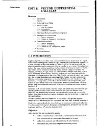
1.6 DERIVATIVE 

You are familiar with notions like velocity, acceleration, slope of a tangent line, 

etc. You also know that differential calculus is the right mathematical tool to 

obtain formulae to calculate velocity and acceleration of moving bodies, the slope 

of the tangent line to a curve, etc. In fact differential calculus deals with the 

problem of calculating rates of change and also helps to express the physical laws 

in precise mathematical terms for studying their consequences. The problems 

associated with a moving body are mainly responsible for development of the 

concept of derivative in calculus. To illustrate the fact we consider the rectilinear 

motion of a body. We know that the distance ‘s’ traversed by the body and 

measured from a fixed point depends on the time ‘t’. Let the distance s = f (t) be a 

function of time ‘t’. The average of velocity during a time interval (t, t + Δt) is 

V av 

Δs 

= , where Δs 

= f ( t + Δt) 

− f ( t). 

Δt 

To obtain the velocity at time t, we need to calculate 

f ( t + Δt) 

− f ( t) 

lim 

Δt 

→0 

Δt 

The above limit, if exists, is called the derivative of f (t) with respect to t and we 

write 

lim 

Δt 

→0 

Δs 

= 

Δt 

ds 

dt 

= f ′ ( t). 

ds 

The derivative is the velocity of the moving body at time t. 

dt

1.6.1 Derivative of a Function 

We now define the derivative of a given function by using the notion of limit. 

Definition 10 

The function y = f (x) is said to have a derivative (or be differentiable) at a 

point x if, and only if, the limit 

lim 

h →0 

f ( x + h) 

− f ( x) 

h 

dy 

exists and is finite. This limit, written as or f ′ (x), is called the 

dx 

derivative of f (x) with respect to x. 

If the derivative of a function exists at every point of an interval, then we say that 

the function is differentiable in that interval. However, while considering the 

derivatives at the end points of an interval, we evaluate suitable one-sided 

derivatives. For example, if the interval is [a, b], then the derivative at x = a is 

calculated as 

lim 

+ 

h →0 

f ( a + h) 

− f ( a) 

and at b as 

h 

lim 

− 

h →0 

f ( b + h) 

− f ( b) 

h 

If f ′ (x) is continuous at a point, then we say that f (x) is continuously 

differentiable at that point. 

Example 1.21 

Solution 

Let y = x n (n is a positive integer). Prove that . 

1 − dy n 

= nx 

dx 

Then 

y = f ( x) 

= 

n 

x 

n 

f ( x + h) 

− f ( x) 

( x + h) 

− x 

= 

h 

h 

( x + h − x) 

−1 

n − 

= 

[ ( x + h) 

+ ( x + h) 

h 

n 2 

The above step is derived by using the result 

We now have 

f 

a 

n 

− b 

n 

= ( a − b) 

[ a 

x 

n 

+ 

. . . 

+ ( x + h) 

x 

b + . . . + ab 

n − 2 n −1 

+ x 

n −1 

n − 2 

n − 2 n −1 

+ a 

+ b 

+ − 

n 

= ( x + h) 

+ ( x + h) 

x + . . . + ( x + h) 

x + x 

h 

( x h) 

f ( x) 

n −1 

n − 2 

n − 2 −1 

Taking the limit h → 0, we get 

dy 

dx 

= 

lim 

h→ 

0 

f ( x + h) 

− f ( x) 

= x 

h 

Therefore, . 

1 − dy n 

= nx 

dx 

n −1 

+ x 

n − 2 

x + 

. . . 

+ x 

n −1 

(n number of terms) 

] 

] 


37


38 

In the following theorem, we make an important observation (a necessary 

condition) about any differentiable function. 

Theorem 5 

Proof 

If a function y = f (x) is differentiable at some point x = x0, it is 

continuous at that point. 

By definition, the derivative of f (x) at x = x0 is 

f ′ ( x ) = 

0 

lim 

h→ 

0 

Now [ f ( x + h) 

− f ( x )] 

lim 0 

0 

h →0 

f ( x0 

+ h) 

− f ( x0) 

h 

f ( x0 

+ h) 

− f ( x0) 

= lim 

. h 

h →0 

h 

= lim 

h →0 

= f ′ ( x0 

) . 0 

= 0 

f ( x0 

+ h) 

− f ( x0) 

. 

h 

∴ f ( x + h) 

− lim f ( x ) = 0 

lim 0 

0 

h →0 

h→ 

0 

i.e. f ( x + h) 

= lim f ( x ) 

lim 0 

0 

h →0 

h→ 

0 

lim 

h →0 

i.e. f (x) is continuous at x0. 

The converse of the above result is not true. Indeed, there exist functions 

which are continuous but not differentiable. 

Example 1.22 

Solution 

Examine the differentiability of the function 

⎧ x whenever x > 0 

y = ⎨ 

⎩− 

x whenever x ≤ 0 

The function is continuous for – ∞ < x < ∞. The graph of the function is 

given below. 

y 

y =− x y = x 

0 

Figure 1.22 

h 

x

Remark 

f ( 0 + h) 

− f ( 0) 

h − 0 

Further = = 1 when h is positive. 

h 

h 

f ( 0 + h) 

− f ( 0) 

∴ = 1 

lim 

+ 

h →0 h 

f 

( 0 

+ h) 

− f 

lim 

− 

h →0 h 

i.e. f ′ (0) does not exist. 

− h − 0 

= = − 1 when h is negative. 

h 

( 0) 

= − 1 

The above example will help you to conclude that a function can never have 

derivative at a point of discontinuity. In the light of this remark, look at the 

following example. 

Example 1.23 

Solution 

Examine the differentiability of the function 

y = x 

y 

⎧ x , 

⎪ 

y = ⎨ 1 , 

⎪ 

⎩3 

− x , 

y = 1 

− ∞ < x < 0 

0 ≤ x< 

2 

2 ≤ x 

y = 3 − x 

0 1 2 3 

Figure 1.23 

From Figure 1.23, we observe as follows : 

(i) The function is not continuous at x = 0. Hence it is not differentiable 

there. 

(ii) Though the function is continuous at x = 2, the one-sided limits 

lim 

+ 

h →0 

= 

f 

( 2 + h) 

− f ( 2) 

h 

lim 

+ 

h →0 

[( 3 

− ( 2 + h) 

] − ( 3 − 

h 

2) 

x 


39


40 

SAQ 6 

and 

lim 

− 

h →0 

= 

= 

= 

= 

lim 

+ 

h→ 

0 

lim 

+ 

h →0 h 

f 

3 − 2 − h − 1 

h 

− h 

= − 1 

( 2 + h) 

− f ( 2) 

h 

lim 

− 

h→ 

0 

lim 

h →0 

− 

1 − ( 3 − 2) 

h 

= 0 = 0 are not equal. 

Therefore, the derivative does not exist at x = 2. 

At all points (x ≠ 0 and x ≠ 2) the derivatives exist. 

(a) Show that the derivative of a constant function is zero. 

(b) Show that y = | x | is differentiable at all points except at x = 0. 

(c) Find the derivative of the function 

(i) y = x 2 

(ii) y = 3x 2 + 5x – 1. 

1.6.2 Algebra of Derivatives 

We now state some important rules regarding the derivatives of the sum, 

difference, product and quotient of functions in terms of their derivatives. 

Theorem 6 

If f (x) and g (x) are differentiable functions at a point x, then 

(i) 

d df ( x) 

dg ( x) 

[ f ( x) 

± 

g( 

x)] 

= ± 

dx 

dx dx

(ii) 

(iii) 

d dg ( x) 

df ( x) 

( f ( x) 

. g ( x)) 

= f ( x) 

+ g ( x) 

dx 

dx 

dx 

d 

dx 

df ( x) 

dg( 

x) 

⎛ 

g ( x) 

f ( x) 

f ( x) 

⎞ 

− 

dx 

dx 

⎜ 

g ( x) 

⎟ = 

2 

⎝ ⎠ 

[ g ( x)] 

provided g (x) ≠ 0. 

We shall give the proof of the result (ii) below. Other results we leave as an 

exercise for you. 

Proof 

Let y = f (x) . g (x) 

Then 

dy 

dx 

= lim 

h→ 

0 

f ( x + h) 

g ( x + h) 

− f ( x) 

g ( x) 

h 

Now f ( x + h) 

g ( x + h) 

− f ( x) 

g ( x) 

∴ 

That is, 

dy 

dx 

dy 

dx 

dy 

dx 

= f ( x + h) 

[ g ( x + h) 

− g ( x)] 

+ g ( x) 

[ f ( x + h) 

− f ( x)] 

⎧ [ g ( x + h) 

− g ( x)] 

[ f ( x + h) 

− f ( x)] 

⎫ 

⎨ f ( x + h) 

+ g ( x) 

⎬ 

⎩ 

h 

⎭ 

= lim 

h→ 

0 

h 

g ( x + h) 

− g ( x) 

= lim f ( x + h) 

lim 

h→ 

0 

h →0 

h 

f ( x + h) 

− f ( x) 

+ g ( x) 

. lim 

h →0 

h 

dg ( x) 

df ( x) 

= f ( x) 

+ g ( x) 

, 

dx dx 

Use of the product rule (ii) and the result which states that ‘derivative of a 

constant is zero’ gives 

d 

dx 

where c is a constant. 

Example 1.24 

Solution 

d 

= [ cf ( x)] 

= c f ( x) 

, 

dx 

Find the derivative of y = 5x 2 sin x. 

dy 

dx 

d 

d 

= 5 [ x (sin x) 

+ sin x ( x 

dx 

dx 

2 2 

d 

We derive (sin x) 

as under : 

dx 

d 

dx 

(sin x) 

= lim 

h→ 

0 

sin ( x + h) 

− sin x 

h 

)] 


41


42 

Solution 

= 

⎛ ⎛ h ⎞ ⎞ 

⎜ sin ⎜ ⎟ ⎟ 

⎛ h ⎞ ⎜ ⎝ 2 

lim cos 

⎠ 

⎜ x + ⎟ 

⎟ 

⎝ 2 ⎠ ⎜ h ⎟ 

⎜ ⎟ 

⎝ 2 ⎠ 

h 

→0 

2 

⎛ h ⎞ 

sin ⎜ ⎟ 

⎛ h ⎞ 2 

= lim cos x lim 

⎝ ⎠ 

⎜ + ⎟ . 

h 

0 ⎝ 2 ⎠ h h 

→ 

→0 

2 

2 2 

= cos x . 1 = cos x 

d 

and ( x ) 2x 

dx 

2 = 

dy 2 

Hence, = 5 [ x cos x + 2x 

sin x] 

. 

dx 

Example 1.25 

dy 

Find , if 

dx 

By formula (iii) 

cos x 

y = . 

2 

x 

dy 

dx 

= 

x 

2 

d 

dx 

d 

To obtain (cos x) 

, we have 

dx 

d 

dx 

(cos x) 

(cos x) 

− cos x 

= lim 

h →0 

= 

h 

→0 

2 

d 

and ( x ) 2x 

dx 

2 = 

Therefore, 

x 

4 

d 

dx 

( x 

cos( 

x + h) 

− cos x 

h 

⎛ 

⎛ h ⎞ ⎞ 

⎜ 

sin ⎜ ⎟ ⎟ 

⎜ ⎛ h ⎞ ⎝ 2 

lim − sin 

⎠ ⎟ 

⎜ 

⎜ x + ⎟ lim 

⎝ 2 ⎠ h h ⎟ 

→0 

⎜ 

2 ⎟ 

⎝ 

2 ⎠ 

⎛ h ⎞ 

sin ⎜ ⎟ 

⎡ ⎛ h ⎞⎤ 

2 

= − lim sin x lim 

⎝ ⎠ 

h ⎢ ⎜ + ⎟ 

0 2 

⎥ h 

⎣ ⎝ ⎠⎦ 

h 

→ 

→0 

2 

2 2 

= − sin x . 1 = − sin x 

dy xsin 

x + 2cos 

x 

= 

dx 

3 

x 

2 

)

1.6.3 Derivative of a Composite Function (Chain Rule) 

Theorem 7 

Proof 

If y = f (u) is a differentiable function of u and u = g (x) is a 

differentiable function of x, then y = f (g (x)) as a function of x is 

differentiable and 

dy 

dx 

dy du 

= . . 

du dx 

Let u = g (x) be differentiable at x0 and y = f (u) be differentiable at u0 

where u0 = g (x0). 

Let h (x) = f (g (x)). The function g (x), being differentiable, is continuous at 

x0; so also the function f (u) at u0 and, therefore, at x0. 

where Δu → 0 as Δx → 0 

and at u0 

Δu = g (x0 + Δx) – g (x0) 

Δy = f (u0 + Δu) – f (u0) 

= f (g (x0 + Δx)) – f (g (x0)) 

= h (x0 + Δx) – h (x0) 

Assuming Δu ≠ 0 (i.e. g (x) is not a constant function in neighbourhood 

of x0), we write 

In the limit, we get 

or 

Δy 

Δy 

Δu 

= . 

Δx 

Δu 

Δx 

Δy 

Δy 

Δu 

lim = lim lim 

x →0 

Δx 

Δu 

→0 

Δu 

Δx 

→ Δx 

Δ 0 

dy 

= 

dx 

dy 

du 

du 

dx 

You can also show that in the case of Δu = 0 the above formula holds true. In fact 

it becomes an identity 0 = 0. Note that it cannot be divided by Δu in the case. 

Example 1.26 

Solution 

If y = sin (x 2 dy 

), find . 

dx 

Let y = sin (u) and u = x 2 . By the chain-rule 

dy 

dx 

= 

d 

du 

(sin u) 

. 

= (cos u) (2x) 

= 2x cos x 2 . 

du 

dx 


43


44 

1.6.4 Second Order Derivatives 

You know that the derivative of a function y = f (x), i.e. f ′(x) is also a function. 

Hence we can calculate the derivative of f ′(x) at a point of its domain, if it exists, 

f ′ ( x + h) 

− f ′ ( x) 

by using the same limiting procedure. That is, if lim exists, it is 

h →0 

h 

called the second order derivative of f (x) with respect to x. We write it as 

2 

d y 

or f ′ ( x) 

. You can also calculate higher order derivatives like 3 

2 

dx 

rd order, 

4 th order etc., of a function f (x). 

Example 1.27 

Solution 

Find the (i) 2 nd order and (ii) 5 th order derivatives of y = x − x + 5x 

− 1. 

(i) 4 6 5 

3 

dy 

= y′ 

= x − x + 

dx 

(ii) 

2 

d y d ⎛ dy ⎞ d 3 

= ⎜ ⎟ = ( 4x 

− 6x 

+ 5) 

= 12x 

2 

dx dx ⎝ dx ⎠ dx 

y 

( 3) 

( 4) 

= 24x, 

y = 24, 

y 

( 5) 

1.6.5 Implicit Differentiation 

6 

= 0 

4 

If we are given an equation like x + 4xy 

− 3y 

+ 1 = 0 , it is not easy to solve it 

dy 

for y in terms of x. However, it is often possible to calculate straight from the 

dx 

equation by the method of implicit differentiation. For example, if we 

differentiate both the sides of the given equation, we get 

Therefore, 

3 

2 

− 6 

5 4 ⎛ 3 dy ⎞ ⎛ 2 dy ⎞ 

6x 

+ 4y 

+ 4x 

⎜4 

y ⎟ − 3 ⎜3y 

⎟ + 0 = 

⎝ dx ⎠ ⎝ dx ⎠ 

dy 

dx 

⇒ 6x 

5 

+ 4y 

5 

4 

+ 

4 

( 16 

− ( 6x 

+ 4y 

) 

= 

3 2 

16xy 

− 9y 

xy 

3 

− 9y 

This holds for all points where 16xy 

− 9y 

≠ 0 . 

SAQ 7 

(a) Differentiate 

(i) 

(ii) 

3x 

+ 1 

2x 

− 5 

x 

3 

1 

+ 3x 

− 8 

3 

2 

2 

) 

dy 

dx 

= 0 

d 

dx 

4 

( 0) 

3 2

(iii) (x 2 + x + 6) sin x 

(iv) (x + 2) (x 2 + 1) + cos x 

(b) Find the derivatives of the functions 

(i) 

2x 

+ 3 

x 

2 − 

(ii) tan x 

(iii) 

( 1 

1 + 

5 

− sin x) 

2 

cos 

x 

(c) Find the 2 nd order derivatives of the functions 

(i) sin 2 x 

(ii) ax 3 + bx 2 + cx + d 

1.6.6 Derivatives of Some Elementary Functions 

Power Function y = x α (α is real) 

We have already proved that the power function y = x n , where n is a 

positive integer, has the derivative 

dy 

dx 

= 

n 

n x 

−1 

We shall show now that the above rule also holds when 

integers with q > 0). 

Let us assume p, q > 0. 

Then y q = x p . By the method of implicit differentiation, we get 

or 

q y 

dy 

= p x 

dx 

q −1 

p −1 

p −1 

p −1 

p 

−1 

dy p x p x p q n 

= = = x = nx 

dx q −1 

p 

q y 

p − q 

q 

q x 

−1 

p 

q 

y = x (q, p are 

, 

if 

p 

q 

= n 


45


46 

d α 

In fact the formula ( x ) = α x 

dx 

accept this result without proof. 

Trigonometric Functions 

We have already seen that 

α −1 

d 

d 

(sin x) 

= cos x, 

(cos x) 

= − sin x 

dx 

dx 

By using the quotient rule you can show that 

d 

dx 

Logarithmic Function 

holds true for any real α. We shall 

2 d 

(tan x) 

= sec x, 

(cot x) 

= − cosec 

dx 

dx 

d 1 

We shall prove that (log x) 

= 

dx x 

Let f (x) = log x 

d 2 

d 

(sec x) 

= sec x tan x, 

(cosec 

x) 

= − cosec 

x cot x 

dx 

f ( x + h) 

− f ( x) 

1 

1 ⎛ h ⎞ 

Then = [log ( x + h) 

− log ( x)] 

= log ⎜1 

+ ⎟ 

h h 

h ⎝ x ⎠ 

f ( x + h) 

− f ( x) 

log ( x + h) 

− log x 

f ′ ( x) 

= lim 

= lim 

h→ 

0 h 

h→ 

0 h 

1 ⎛ h ⎞ 

= lim log ⎜1 

+ ⎟ 

h →0 h ⎝ x ⎠ 

= lim 

h →0 

⎛ h ⎞ 

log ⎜1 

+ ⎟ 

⎝ x ⎠ 1 

. 

h x 

x 

⎛ h ⎞ 

log ⎜1 

+ ⎟ 

x 1 1 1 

= lim 

⎝ ⎠ 

. lim = 1 × = 

h →0 

h h →0 

x x x 

x 

or ⎟ ⎛ log ( 1 + y) 

⎞ 

⎜ 

⎜∵ 

lim = 1 

⎝ y →0 

y ⎠ 

Exponential Function (with respect to the base a) 

We shall now prove that 

d 

dx 

Let y = a x . 

x 

x 

( a ) = a log a . ( a > 0 but a ≠ 1) 

Then loge y = x loge a 

By the method of implicit differentiation, we get 

1 

y 

dy 

dx 

= 

loge 

a 

e 

x

dy 

x 

Therefore, = y log e a = a loge 

a 

dx 

In particular if y = e x , then 

Inverse Function 

Let y = sin – 1 x 

Then sin y = x 

dy 

= 

dx 

x 

e 

Differentiating both sides w. r. t. x, we have 

i.e. 

dy 

cos y = 1 

dx 

dy 

dx 

= 

= 

= 

= 

1 

cos 

y 

1 

2 

cos 

1 − 

1 

1 

1 − x 

y 

2 

sin 

2 

−1 π π 

As we know that the range of sin x is − to , i.e. y lies between 

2 2 

π 

to 

2 2 

π 

− , so cos y is positive. 

Similarly, 

Example 1.28 

Let 

Solution 

y = 

dy 

Find . 

dx 

= − 

dx 

cos 1 − 

y = cos 

y = tan 

y = cot 

−1 

−1 

−1 

x ⇒ 

x ⇒ 

x ⇒ 

dy 

dx 

dy 

dx 

dy 

dx 

π π 

(tan x) 

, − < x < 

4 4 

y 

= − 

d 

(tan x) 

= − 

x) 

dx 

1 

= 

1 + x 

1 

1 − x 

2 

1 

= − 

1 + x 

dy 1 

1 

2 

= − 

( 1 

− tan 

1 

2 

cos x cos 2x 

( 1 

2 

2 

sec 

2 

− tan x) 

x 


47


48 

1.6.7 Derivatives of a Function Represented Parametrically 

Sometimes we represent a function say y = f (x), a ≤ x ≤ b by its parametric 

equations, 

x = φ( 

t) 

⎤ 

y = ψ t 

⎥, 

( ) ⎦ 

α ≤ t ≤ β 

Let us assume φ (t), ψ (t) are differentiable and x = φ (t) has an inverse t = h (x). 

Then we can consider the equation of the function y = f (x) as a composite 

function. 

y = ψ( 

t), 

t = h( 

x) 

Using the differentiation rule for a composite function (chain-rule), we get 

dy 

dx 

dy 

= . 

dt 

dt 

dx 

dψ 

= 

dt 

dh 

dx 

dψ 

= 

dt 

dφ 

dt 

Since t = h (x) is inverse of x = φ (t), we arrive at 

Example 1.29 

dy 

dx 

dψ 

= 

dt . 

dφ 

dt 

The parametric equation of a semi-circular arc of radius ‘a’ with its centre 

at (0, 0) is 

Find 

Solution 

dy 

dt 

x = a cos t⎤ 

y = a t 

⎥, 

sin ⎦ 

π 

at t = . 

4 

dy 

dx 

= 

dy 

dt 

dx 

dt 

0 ≤ t ≤ π 

a cos t 

= = − cot t 

a( 

− sin t) 

π dy π 

At t = , = − cot = − 1 

4 dx 4 

1.6.8 Logarithmic Differentiation 

In some problems, it is easier to find dx 

dy by first taking logarithmic and then 

differentiating. Such process is called logarithmic differentiation. This is usually 

done in two kinds of problems. First when the function is a product of many 

simpler functions. In this case logarithm converts the product into a sum and

facilitates differentiation. Secondly, when the variable x occurs in the exponent. 

In this case logarithm brings it to a simpler form. 

Example 1.30 

Solution 

Solution 

Differentiate sin x sin 2x sin 3x. 

Let y = sin x sin 2x sin 3x 

Then log y = log sin x + log sin 2x + log sin 3x. 

Differentiating both sides, we have 

1 

y 

dy 

dx 

= 

1 

1 

1 

. cos x + . cos 2x 

. 2 + . cos3x 

. 3 

sin x sin 2x 

sin 3x 

dy ⎡cos 

x 2cos 

2x 

cos3x 

⎤ 

∴ = y ⎢ + + 3 ⎥ 

dx ⎣ sin x sin 2x 

sin 3x 

⎦ 

Example 1.31 

Differentiate (sin x) x 

Let y = (sin x) x 

Then log y = x log sin x 

= sin x sin 2x sin 3x [cot x + 2 cot 2x + 3 cot 3x] 

Differentiating both the sides, we have 

1 

y 

dy 

dx 

= log sin x + x . 

1 

. cos x 

sin x 

dy 

i.e. = y [log sin x + x cot x] 

dx 

= (sin x) x [log sin x + x cot x] 

1.6.9 Differentiation by Substitution 

Sometimes it is easier to differentiate by making substitution. Usually these 

examples involve inverse trigonometric functions. 

Example 1.32 

Solution 

− 

Differentiate ⎛ 

⎞ 

⎜ + x − x⎟ 

⎝ 

⎠ 

2 

1 

tan 1 

Put x = tan θ 

Then 1 + x 2 = sec 2 θ 


49


50 

2 

∴ 1 + x − x = secθ 

− tan θ 

= 

1 sin θ 

− 

cosθ 

cosθ 

1 − sin θ 

= 

cosθ 

cos 

= 

⎛ π θ ⎞ 

∴ tan y = tan ⎜ − ⎟ 

⎝ 4 2 ⎠ 

i.e. 

2 

θ 2 θ θ θ 

+ sin − 2sin 

cos 

2 2 2 2 

2 θ 2 θ 

cos − sin 

2 2 

⎛ θ θ ⎞ 

⎜cos 

− sin ⎟ 

⎝ 2 2 

= 

⎠ 

⎛ θ θ ⎞ ⎛ θ θ ⎞ 

⎜cos 

− sin ⎟ ⎜cos 

+ sin ⎟ 

⎝ 2 2 ⎠ ⎝ 2 2 ⎠ 

θ θ θ 

cos − sin 1 − tan 

⎛ π θ ⎞ 

= 2 2 = 2 = tan ⎜ − ⎟ 

θ θ θ 

cos + sin 1 + tan ⎝ 4 2 ⎠ 

2 2 2 

π θ 

y = − 

4 2 

dy 1 dθ 

1 d −1 

∴ = − = − (tan x) 

dx 2 dx 2 dx 

SAQ 8 

= 

2( 

1 

− 1 

+ 

2 

x 

) 

(a) A particle moves along a straight line. At any time t the distance s 

travelled by the particle is given by the formula : s = 32t 2 + 9. Find 

the velocity and acceleration of the particle at time, t = 2 units. 

dy 

(b) Use the method of implicit differentiation to calculate , if 

dx 

2 

2x 

− 3xy 

+ 4y 

2 

= 8 

2

(c) Differentiate the following 

(i) x 2 e x sin x 

(ii) (x + 1) 2 (x + 2) 3 (x + 3) 4 

(iii) 

tan 

−1 

2x 

1 − x 

2 

−1 

1 − x 

(iv) cos 

2 

1.7 SUMMARY 

1 + x 

In this unit, we have covered the following points : 

2 

• The absolute value of a real number x, written as | x |, is defined as 

⎧ x 

| x | = ⎨ 

⎩− 

x 

if 

if 

x ≥ 0 

x < 0 

• Various types of intervals in R are : 

open : (a, b) {x ∈ R : a < x < b} 

closed : [a, b] = {x ∈ R : a ≤ x ≤ b} 

semi-open : (a, b] = {x ∈ R : a < x ≤ b} 

semi-closed : [a, b) = {x ∈ R : a ≤ x < b} 

• A function of f : x → y is said to be onto (or surgective) if range 

of f = y. 

• A function of f : x → y is said to be one-one (or injective) if 

f (x1) = f (x2) ⇒ x1 = x2. 

• A function f is said to be even if f (− x) = f (x), and odd if 

f (− x) = − f (x). 

• lim f ( x) 

= l , if and only if, lim f ( x) 

= l = lim f ( x) 

. 

x → a 

+ 

x →a 

− 

x → a 

• f is continuous at x = a if, and only if, lim f ( x) 

= f ( a) 

. 

x → a 

f ( x + Δx) 

− f ( x) 

• f (x) has the derivative at x if lim 

x →0 

Δx 

d 

d d 

• [ α f ( x) 

+ β g ( x)] 

= α f ( x) 

+ β g ( x) 

. 

dx 

dx dx 

d 

d 

d 

• [ f ( x) 

g ( x)] 

= f ( x) 

g ( x) 

+ g ( x) 

f ( x) 

. 

dx 

dx 

dx 

• 

d 

dx 

⎡ 

g ( x) 

f ( x) 

⎤ 

⎢ ⎥ = 

⎣ g ( x) 

⎦ 

d 

dx 

f ( x) 

− f ( x) 

2 

[ g ( x)] 

d 

dx 

g ( x) 

. 

exists. 


51


52 

• If y = f ( u) 

and u = g ( x) 

, then 

d n 

• 

n 

( y ) = ny 

dx 

−1 

dy 

. 

dx 

• 

dy g′ 

( t) 

If x = f ( t), 

y = g ( t), 

= . 

dx f ′ ( t) 

dy 

dx 

dy du 

= . . 

du dx 

• If f (x) is differentiable at x = c, then it is continuous at x = c. 

1.8 ANSWERS TO SAQs 

SAQ 1 

SAQ 2 

SAQ 3 

SAQ 4 

(b) (i) False 

(ii) True 

(iii) True 

(iv) False 

(b) (ii) and (iii). 

(c) (i) and (iv). 

(d) 

y + 1 

x = is the inverse. 

y − 1 

(c) (i) even 

(i) 

(ii) even 

(iii) even 

(iv) even 

(v) neither even nor odd. 

2 

x − x − 6 ( x 

= 

2 

( x + 2) 

− 3) 

( x 

( x + 2) 

(ii) The limit does not exist. 

(iii) Limit is 0 as 

(iv) Limit is 1 as 

(v) Limit 

2 

= − . 

3 

( x 

(vi) Limit does not exist. 

(vii) Limit does not exist. 

2 

+ 

2 

2) 

− x − 12) 

x − 3 

2 

= 

x 

x 

− 

+ 

3 

2 

= ( x − 

tan x sin x 1 

= . . 

x x cos x 

3) 

, so the limit does not exist. 

( x + 

4) 

2 

.

SAQ 5 

SAQ 6 

SAQ 7 

SAQ 8 

(viii) Limit 

(ix) Limit 

= 

1 

. 

2 3 

α 

= . 

β 

(a) (i) Not continuous at x = 0 and continuous at all other points. 

(b) b = 4. 

(ii) Not continuous. 

(c) (i) 2x 

(a) (i) 

(b) (i) 

(ii) 6x + 5 

( 2 

− 

x 

17 

2 

− 5) 

2 

3x 

+ 3 

(ii) − 

3 

2 

( x 

+ 3x 

− 8) 

(iii) (x 2 + x + 6) cos x − (2x + 1) sin x 

(iv) x 2 + 1 + 2x (x + 1) – sin x 

− 2x 

2 

( x 

(ii) sec 2 x 

(iii) 

(c) (i) 

2 

− cos x 

2 (sin 

2 

− 6x 

− 10 

− 

( 1 

(ii) 6ax + 2b 

(a) Velocity = 128 

(b) 

5) 

2 

+ cos 

x − cos 

Acceleration = 64 

dy 

dx 

4x 

− 3y 

= 

3x 

− 8y 

2 

2 

x) 

− 

( 1 

x) 

( 1 

+ cos 

2 x ⎛ 2 ⎞ 

(c) (i) x e sin x ⎜ + 1 + cot x⎟ 

⎝ x ⎠ 

− sin x) 

( − 2 cos x sin x) 

2 

x) 

2 3 4 ⎡ 2 3 4 ⎤ 

(ii) ( x + 1) 

( x + 2) 

( x + 3) 

⎢ + + ⎥ 

⎣ x + 1 x + 2 x + 3⎦ 

(iii) 

(iv) 

2 

1 + x 

2 

1 + 

x 

2 

2 

2 


53


54

MATHEMATICS-II 

The knowledge and concepts of mathematics help in handling any engineering 

problem. In Mathematics-I, you have studied some topics on Algebra, 

Trigonometry, Coordinate Geometry and Vector Algebra. In Mathematics-II, 

which is in your hands, you will be studying some more concepts of mathematics 

which are a must for you. Mathematics-II will be dealing with the concepts of 

Differentiation, Integration, Complex Numbers, Matrices, Determinants and 

Statistics and consists of seven units. 

Units 1 and 2 are devoted to Differential Calculus. In fact, calculus was created to 

meet the pressing mathematical needs of 17th century for solving problems in 

Science and Technology. 

In Unit 1, the concept of function has been introduced and different types of 

functions and inverse functions have been discussed. This unit also lays the 

foundations of calculus in terms of definitions and theorems centering around 

limit and continuity of functions and algebra of derivatives. 

In Unit 2, we will be dealing with some of the applications of the derivatives to 

geometry and maxima and minima of functions. Some important theorems 

namely Rolle’s Theorem and Lagranges Mean-value Theorem have also been 

discussed to understand the concept of increasing and decreasing functions. 

Unit 3 and 4 deal with the concept of integrals and its applications. 

In Unit 3, indefinite integral of a function as an antiderivative has been defined 

and deals with the different techniques for finding integrals of functions. 

In Unit 4, the concept of definite integral has been introduced and some 

applications have been dealt such as finding the area of a curved surface. 

Unit 5 deals with the concept of complex numbers and its properties. The 

important De-Moiver’s theorem has also been discussed. 

Unit 6 deals with the algebra of matrices and the properties of determinants. 

Inverse of a matrix has been discussed and how it is used to solve a system of 

linear equations. 

In Unit 7, statistics, methods for collection of data, construction of frequency 

tables have been discussed. Mean and median measures of location and standard 

and mean deviation have been defined to analyse the information collected. 

For the want of clarity in concepts, number of solved examples have been 

introduced in each unit. To help you check your understanding and to assess 

yourself, each unit contains SAQs. The answers to these SAQs are given at the 

end of each unit. We suggest that you look at them only after attempting the 

exercises. 

At the end, we wish you all the best for your all educational endeavours. 


55

unit 1 differential calculus - IGNOU

Create successful ePaper yourself

Delete template?

Save as template?