UNIT 11 VECTOR DIFFERENTIAL CALCULUS - IGNOU

Vector Calculu~
UNIT 11 VECTOR DIFFERENTIAL
CALCULUS
Structure
11.1 Introductio~i
Objectives
11.2 Scalar and Vector Fields
11.3 Vector Calculus
11.3.1 Limit and Continuity
11.3.2 Differentiability
11.3.3 Applications of Derivatives
11.4 Directional Derivative and Gradient Operator
11.5 Divergence of a Vector Field
11.5.1 Physical Interpretation
11.5.2 Formulae on Divergence of Vector Functions
11.6 Curl of a Vector Field
11.6.1 Physical Interpretation
11.6.2 Rotation of a Rigid Body
11.6.3 Formulae on Curl, Divergence and Gradient
11.7 Summary
11.1 INTRODUCTION
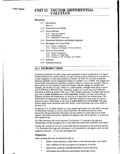
In physical problems we often come across quantities such as temperature of a liquid,
distance between two points, density of a gas, velocity a~id acceleratio~i of a particle or
a body, tangent to a curve and normal to a surface. In Unit 10, you have learnt that
physical quantities can be categorised either as a scalar or as a vector. You might have
noticed that some physical quantities, whether scalars or vectors, are variable. That is,
their values are not constant or static but change with the change in variable. For
example, the density of a gas, which is a scalar quantity, changes from place to place
and is different at different times. Similarly, tangent to a curve may have different
directions at different points of the curve. This variable character of scalars and vectors
give rise to scalar functions and vector functions. Further, you may notice that at
different positions the temperature or velocity of a body does not remain same. The
distribution of temperature or velocity is therefore defined at each point of a given
domain in space which leads to the idea of scalar fields aiid vector fields. We shall
discuss about scalar functions and scalar fields, vector functions and vector fields in
Section 11.2.
In Section 11.3, we shall extend, in a very simple and natural way, the basic concepts
of differential calculus to vector-valued functions. We shall also discuss about
physically and geometrically important concepts related to scalar and vector fields
namely, directional derivatives, gradient, divergence and curl in Section 11.4 and give
their applications.
We shall introduce the vector operator V in Sectioii 11.5 and give the physical
interpretation of the divergence of a vector field and some basic formulas involving it.
Finally, the concept of curl of a vector field and its invariance is discussed in Section
11.6. Formulas involving curl, divergence, curl and gradient, divergence and curl and
Laplacian operator, v2, are also developed here.
Objectives
After studying this unit you should be able to
* define a scalar function, a scalar field, a vector function and a vector field,
* state coilditions for the coilvergence of a sequence of vectors,
* define limit, continuity and differentiability of vector functions,
* differentiate sum, difference and products iilvolvi~lg vectors,

* describe the notion of directional derivative and compute directional Vector DLlltmatial Calculus
den va tives,
* define and compute gradient of a scalar field and divergence and curl of vector
fields,
* interpret physically the gradient, divergence and curl of a vector,
* define conditions for solenoidal and irrotational vector fields, and
* solve problems on application of del operator and product rules involving the
del operator.
11.2 SCALAR AND VECTOR FIELDS
Let us first talk about the scalar field.
Scalar Fields : Consider the distance of a point P from a fixed point Po which will be a
real number. As we vary the point P its distance from Po also changes. It depends only
on the location of point P in space and may be regarded as function f (P). If we
consider cartesian coordinate system in space and take coordinates of fixed point Po as
(x,, yo, zo) and the variable point P as (x, y, z), then f is given by the well-known
f(P) = f(x.y,z) = \/(x - x")~ + (y -
+(z -1")'.
Next, consider a room fitted with an air-conditioner (A.C.). Once A.C. is switched on
for its cooling effect; the temperature of room falls down. Now, if we put off the A.C.,
the temperature starts rising up till it reaches the room temperature. The temperature
further rises up if we now switch on the A.C. for its heating effect.
Thus, the temperature of the room depends on the switching system of the air
conditioner.
In this case, the temperature of the room can be considered as a function of switching
system of the A.C.
In both the examples taken above, you may note that distance, as well as, temperature
give us only the magnitude and not the direction. Hence both are scalar quantities.
These quantities depend either on the position of P or on the switching system of the
A.C. In both the situations, we get a function. Functions of this type are called Scalar
Functions. It may also be noted here that distance or temperature functions do not
depend on the choice of coordinate system or brand of A.C., but only on the physical
situations such as actual distance or actual duration of switching on the A.C.
Formally, we give the following definition of a scalar.
Definition : A Scalar function is a function which is defined at eacli polnt of certai~z
region (domain) in space and whose values are real numbers depending only on the
points in space but not on particular choice of the coordinate system.
In most of the applications, the domaill of a scalar function is a curve, a surface, or a
three-dimensional region in space.
In the case of temperature of a room fitted with A.C., the do~nain of temperature
function is the set of points on the regulator of A.C., which controls the temperature of
the room.
The function f associates with each poiut in domain D a scalar (a real number) and we
say that a scalar field is obtained in D. More formally, we hgve the following
definition :
Definition : If i) be a function which associates a unique scalar with eacli point in a
given region, then $ is called a scalar field function, or simply a scalar field.
In a plane, for instance, the equation of a curve is given by f (x, y) = constant, i.e.,
these are curves along which f has a constant value for all points in the x y - plane.
Similarly, a surface may be given by i) (x, y, z) = constant, i.e., these are surfaces for
which i) has a constant value for all points in space. In these examples scalar functions .
f and i), having plane and space as their respective domains, are scalar'fields.
Some more examples of scalar fields are the density of the air of the earth's atmosphere
and the pressure within a region through which a compressible fluid is flowing.

Vector Calculus
We can represent a scalar field by a formula as well as pictorially. For a pictorial
representation, we may use the curves and surfaces. The pictorial representation of
scalar fields are maps showing physical geography of a region (indicating hills, lakes,
land above or below sea level, etc.).
In the same manner when we assign a vector to each point of a certaill region we obtain
a vector field. Let us now talk about vector fields.
Vector Fields
Consider a curve in a plane or in space. At each point of the curve we can draw a
Figure 11.1 : Tangent Vectors of a curve Figure 11.2 : Normal Vectorsofa surface
A
We can assign to each point P of the curve, a tangent vector t (P) (see Figure. 11 .I).
Similarly at each point of a surface, we can draw a nornlal (see Figure 11. 2). These
llormals inay have different directions at different points of the surface. Thus to each
A
point Q of the surface, a nonnal vector n ( Q ) lnay be assigned.
Moreover, a vector may depend on one or more than one indepeildent scalar variables.
The velocity of a particle, for instance, depelids on the position of the particle as well
as time. The same is true for position vector and acceleration of a particle.
We now give the following definition :
Definition : If to each point P of n certain region G in spnce a vector V (P) is
assigrted, then V (P) is called n vector function.
There are many examples of vector functions ill physics. For example velocity,
acceleration, and forcc are all vector functions. The gravitational force exerted by the
sun on a unit mass is also a variable vecto~, depending on the position of the mass, and
thus represents a vector function.
The collectio~l of all such vector fuilctio~ls V (P) is called a vector field on G. More
precisely, we give the following definition :
Definition : IfF be a function which assigns to each point x in its domain, a vector
F (x) is called a vector field function or a vector field.
A physical exaillple of vector field is given by the particles of a fluid under flow.
At any instant the velocity vector V (P) of a rotatilig body collstitutes a vector field,
called the velocity field of rotation. If we introduce a cartesian coordinate system
having the origin on the axis of rotation, then
A L A
V(x,y,z) = LI) x (xi + y j + zk),
where r, y, z ate the coordinates of any point P of the body in a plane perpendicular to
the axis of rotaltion and o is the rotation vector or constant angular vclocity of the body
(see Figure 11.3).
Next consider a particle A of inass M, which is placed at a fixed point Po and let a
particle B of mass m be free to take up various positions P in space (see Figure 11.4).

' axis
- 1
of rotation
Figure 11.3. Velocity Field of a body rotating with consmat angular wlocity O in
the positive (counter clockwise) di~ction
I b
Then particle A attracts particle 8. According to Newton's law of attractionlgravitation,
the corresponding gravitational force p is directed from P to Po and its magnitude is
1
proportional to -, where r is the distance between P and Po. Then
r2
GMm
IpI=--p
where G is the gravitatio~ial constant. Hence p defi~ies a vector field in space.
0
Vector Differential Cak
Figure 11.4 Some of the vecton of gravitational field
By now you must have clearly understood what we mean by scalar functions, scalar
fields, vectors functions and vector fields. You can test your knowledge by attempting
the following exercise :
E 1.
Which of the followillg are scalar functioils, scalar fields, vector fu~~ctiorls and vector
fields ?
(a)
(b)
(c)
(d)
(e)
The gravitational force on a particle of mass Mat distance r due to
another particle of mass m.
A collstant force applied to a particle.
The temperature at every point of a mass of heated liquid.
Potential of an electric charge placed at the origin.
The force on a unit charge placed at a point P due to an electric charge
e placed at the origin.
You have already learnt about the basic concepts of limit, continuity, differentiability
and partial differentiation of scalar fuiictio~ls in Units 2 and 5 of Block-I. We shall
now, in the next section, illtroduce these basic concepls of calculus for vector functiolls
in a simple and natural way.
11.3 VECTOR CALCULUS
We begin by introducing the idea of limit and continuity of a vector function. We
know that the limit concept is a basic and useful tool for the analysis of functions. It
enables us to study derivatives, improper integrals and other important features of
W ball inlrodu[c Ihc mlcepls of limit and co~~tinuity
~unctions, e s
manner without going into the intricaciof delta, epsilon method.
* A 4 1 !-.-!A -...I
c#.-4:...-:4 --
~II
a most informal

Vector Calcu11~
the length and direction of I. more precisely, we define \;mite of v-c*o* raluca
functions in te- of the familiar limits of real-valued functions in the following way.
A A A
Definition : Let f ( t ) - fi ( t ) i + f2 ( t ) j + f3 ( t ) k be a vector valued function oft
defined in some reighbourhood of a (possibly except at a). The limit off ( t ) as t
approaches the number a is the vector 1 #the limit of I f ( t ) - 1 1 as t approaches a is
zero. In symbols
l==lim f(t)elim If(t)-11 -0
I-a r-a
Observe that f ( t ) having las a limit means that the components off have the
corresponding components of 1 as limits. In other words, if
then
f )
= f )
- A b
A
i + f2(t) j + f3(t).2 and 1 ll i + 123 + l3 i
lim f(t) = 2- lirn fi = 11, lim f2 - I2 and lirn J; = I3
This equivalence says that we may calculate limits of vector- valued functions
componentwise, i.e., one component at a time.
The limit of a vector valued functions can also be defined in the usual 6, E lnani~er as
we do for the real-valued functions in the following way :
A vector function f (t) of a real variable t is said to tend vector 1 as t approaches a, if
to any pre-assignedpositive number E, however small, there corresponds a povitve
number 6 such that
I f (t)-I(c.rwhen)t-a1

In view of the equivalence ia equation (1 1.2) above, we may say that f ( t ) is
continuous at t = a if each component off is continuous at t = a. Thus we may test a
vector function for continuity by applying our knowledge of real-valued functions to
each component of$
Also f (t) is continuous function if it is continuous at every point of its domain.
Just as in the case of real valued functions the sum, the difference, scalar product and
vector product of two continuous vector functions are also continuous. We shall not be
proving these results here. You can check them yourself,
Let us consider the following example :
Example 2 :
Discuss the continuity of the function
Solution :
The function f (t) is continuous at every value oft > 0 because each colnponellt is
continuous fort > 0. However, f is discontinuous fort s 0 because -, 1 the first
di
component off, is not defined fort s 0.
You may now try the following exercises :
E2
Find lim f ( t ) if
1-0
b)
A A A
f(t) = (efsint)i + (efcost)j - e'k
t A 1-cost 1
C) At) = - i + J + i
sin t t
At what values oft are the following vector functions f (t) continuous.
A A A
a) f(t) - (cost)i+ (sint)j + k
In mechanics, if the position vector of a particle is given by r (t) and if we wish to find
its velocity, we will have to differentiate r(t) with respect to time. Similarly, if the
potential of an electric charge is given, then to determine force due to a,n electric
charge, we shall have to take a recourse to differentiation. We now discuss the
~'tC-,,t:,+:~~ nf 9 vector function.
Vector Diiltcrentid Calculus

0
* -
Figure 11.5 : Derivative of a vector
hnction
11.3.2 Differentiability
We define the derivative of a vector-valued function f (t) at a point t = a by the same
type of limit equation as we use for scalar functions. Thus
j'(a) = h--0 ~ i m f ( ~ h + ~ ) - f ( ~ ) ,
provided the limit on the right exists. We then expect that f is differentiable at t = a iff
each of its components is differentiable at t = a. In this connection we prove the
following fqsult :
Theorenl 1 :
A A A
A vector function f ( t ) = f, ( t ) i +fi ( t ) j +f3 ( t ) k is differentiable at t = a iff
each of its component function is differentiable at t = a. If this condition is met, then
Proof :
Consider the difference quotient
f(a+h)-f(a)
h
..
!(a) =i,(a):+ha)j +h(a)P
The left hand side of equation (11.6) has a limit as h + 0 iff each component on the
right hand side has a limit as h -, 0. The ith component on the right has a limit iff fi is
differentiable at a.
Finally, if each component is differentiable at a, then taking the limit h + 0 in equation
(11.6) of each of the quotient, we get equation (11.5), thus proving the result.
I
Note that the differential coefficient f ( a ) is itself a vector and is called the derivative
of f (t) at t = a. From the definition it is clear that every derivable vector fu~lctio~~ is
continuous. Consider the followi~lg example :
Example :
Obtain the derivative off( r ) = ( sid t ) ; + (In t ); + tan- ' (3t ) ;
Solution :
The function and its derivative are defined at every positive value of r.
\
We now give the geometrical interpretatipn of the derivative at a vector valued
function.
.Geometrical Representation of Derivative
Draw the vector f (t) forvalues of the indepellJellt variable t in some interval
co~ltai~ling t and t + A t from the same initial point 0. The11 the locus of head of
nti~ig f for different values oft traces out a space curve (See
and OQ = f (t + A t), then
f(t+At)-f(t) = OQ-OP = PQ = AS,(say).
a lim
dt A,-oAt

The direction of uis the limiting directioq of of A/: But as Q tends top, PQ
d t At
tends to the tangent line at P. Hence the dimtion of gis along the tangelit to the
d t
space curve traced out by P. Lets denote the length of the arc of this curve from a
fixed point on it upto P. Then the magnitude of gis given by
d t
since the ratio IL?fl, chOrdpQ -1 a, At-0,
As arc PQ
Thus derivative of a vectorfunction represetzts a vector whose direction is tangent to
ds
tlre space curve traced by tlre vectorfurtction arzd the magrzitude is -, whm s is the
d t
arc length from a Fred point on the curve to the variable point representing tlre
vector function.
You may note here that a vector will change if either its magnitude changes or
direction changes or both direction and magnitude changes. Jn this regard. the
following results may be remembered :
df
(a) The necessary and sufficient condition for f (t) to be constant is - = 0.
d t
(b) The necessary and sufficient condition for f (t) to have constant magnitude is
(c)
1 he necessary and sufficie~it co~iditioll forf (t) to have constailt/uni€orm
directioii is
The familiar rules of differentiation of real functions yield corresponding rules for
differentiating vector functions; for example,
(i) (cf)' = cf (Caconstant).
I I I
(ii) (u v) = u * v
du
(iii) ( u f ) = - f + u (u is a scalar function of t).
dl dl
I I I
(iv) (u.v) = u .v + u.v
I I I
(v) (uxv) = u XV+UXV
In (v) above the order of the vectors must be carefully observed, as cross multiplication
of vectors is not commutative.
The chain rule of differentiation is also valid for vector valued functioils. That is, if
f (t) is a differentiable functioii of t, aild t = g (s) is a differentiable function of s, then
the composite function f (g(s)) is a differentiable function of s and
We call write equation (1 1.7) in the form
Vector DUlcreathl Calculus

Vector Calculus The chain rule given for vector functions by equation (1 1.8) is an immediate
consequence of the chain rule for scalar functions that applies to the components f,, f,
and f3.
Consider the following example :
Example 4 :
~x~ress~intermsofsif~ (t)=; + sin(t+l)J? + et+ 'i and
ds
t - g (s) - 2-1.
Solution :
From the chain rule we have
We would obtain the same result if we first substitute t = g ( s ) - 2 - 1 in the
formula for f (t) and then differentiate w.r.ts.
And now a few exercises for you.
E4
Find the derivative of the vector function f (t) in each case and give the
domain of the derivative :
(a) f (t) = eZAt + A t e- A j
(b) f(t) = i + 3j-k
(c) f(t) -;sin- '2r +J? taa13t + k -
As we have already mentioned, not all vector functions are functions of one variable.
The velocity of a fluid particle in motion is a function of time and position. The
position vector of a fluid particle at any time and at any position is a vector function of
four variables x, y, z and t. Thus, in any physical problem involving a vector function
of two or more scalar variables, we may be required to find the partial derivatives of

this vector function. In other words, we may be required to find the derivative of the Vtar ~ i ~ ~ ~ C.I~I,,~ t i . 1
vector function w.r.t. one scalar variable treating the other scalar variables as constant.
Partial derivatives can be calculated for vector functions by applying the rules we
already know for differentiating vector fuactions of a siagkscalar variable.
If a vector function f (u, v) be a differentiable function of iwo scalar variables U, v
given' in the component form as
then partial derivatives off w.r.t. u and v are denoted by
respectively and are defined as
?
%,
af 1 af2 1 ah A
-=- r+-J+-k
au au a u a u
and a f afl t af2 1 ah A - - --r+-J+-k
av av a v a v
Similarly, aZ J a2 fl A a2 f2 1 aZh A
- = -- i + ~ j + ~ k
a u2 a u2 a u
etc. are the second order partial derivatives.
a2f a2fl: a2j+ aZf3 A
-=- r+- j+auav
auav auav auav k
The derivatives a2f a2j :
auav avau
are called mixedpartial derivatives and they are equal if each of them is a continuous
function.
Physically, a gives the rate of change 0ffw.r.t. to u at a given point (u,v) in space.
a u
Thus, partial derivatives
of a function f (x, y, z, t) give us the rate of change off in the directions of x, y, z axes at a
given instant and ugives the rate of change off with respect to time at a given point in
at
space.
Consider the following example :
Example 5 :
A A
4
Find the first order partial derivatives of r ( t, , t2 ) = a cos tl i + a sin tl J + t2 k
Solution :
A A
a r
We have - = - a sin tl i + a cos'tl j
a tl
Note that r (tl, t2) is a position vector. It represents a cylinder of revolution of radius a,
having the z- axis as axis of rotation.

Vector Calculus
F i 11.6 Pammebic
Repmentation
of a curve
X Y
Figore 11.7 : Parametric
Representation of Straight lie
Figure 11.8 : Representatiota
of the tangent to a m e
You may now try the following exercise :
E L For each of the vector functionf, find the first partial derivatives w.r.t. x,y,z.
A A
(a) f=xyi+yzj
i
A A
(b) f = #i- e-"j
(c) f - ~ ~ ; + ~ 2 3 + ~ i
You know that curves occur in many considerations iq calculus as well as in physics,
for example, as paths of moving particles. Let us consider some basic facts about
kurves in space as an important application of vector calcuhs about which we are
going to talk in our next section.
1 1.3.3 Applications of Derivatives
The simplest application of vector calculus is some basic facts about curves in space.
Given a cartesian coordinate system, we map represent a curve C by a vector futiction~
A A A
r(t) = x(t)i + y(t)j+ z(t)k.
Here to each value of the real variable t, there corresponds a point of C having
position vector r (to). (see Figure 11.6).
For example, any straight line L can be represented in the fonn
r(t) = a + tb,
whete a and b are contant vectors and line L passes through the point A with position
vector r = a and has the direction of b (see Figure 11.7).
The vector function
A A
r(t) = acosti + bsintj
represents an ellipse in the xy-plane with centre at origin and axes in the directions of
x and y axes.
Further, if a curve C is represented by a continuously differentiable vector functioi~
r (t), where t is any parameter, then the vector
drr - lim r(t+At)-r(t)
dl At--0 At
has the direction of the tangent to the curve C at P (t) (see Figure 11 3).
Thus, the position vector of a point on the tangent is the sum of the gosition vector r
of a point. P on the curve and a vector in the direction of the tangent. Hence the
parametric representation of the tangent is
.

dr
where both r and -depend on P and the parameter o is a real variable.
dt
Let us now consider the following example :
Example 6 :
If a (t) be a variable unit vector, show that
do
(i) - is a vector normal to a.
d t
Solution :
(i)
da
(ii) - is a unit normal vector to a, 0 being the angle through which a turns.
d0
Since a (t) is a unit vector,
Differentiating Eqn. (1 1.9) w.r.t tot, we get
da da
So a and - are at right angles, i.e., - is a vector normal to a.
dt dt
(ii) Let OP = a and OQ = a + A a be two neighbourirrg values of the given
vector making an angle A0 with each other (Figure 11.9).
Then
and
da A a
- = lim -
d0 ~e-oA8
Since Aa is nonnal to a in the limiting position when A0 -. 0, therefore
do
- is normal to a
d0
Also
da
Hence - is a unit vector normal to a
d0
Let us now look into some of the applications of derivatives to dynamics.
Let the position vector of a point moving on a curve be given by 4t). Its
displacement in time At is
Since the velocity V of the moving point is the rate of change of its
displacement w.r.t to time, therefore
Again, the acceleration of the point, being the rate of change of velocity, is
given by
0 a P
Figure lL9

Vector Calculus
f' *
72
1~
Consider the following examples :
Example 7:
Show that if r = a sin ot + b cos ot, where a and b are constants, then
Solution :
We haver=asino t + bcosot
Differentiating w.r.t. tot, we get
d2 r 2 dr
- = - o r and r x - = - a) (a x b).
d t2 dt
and dZr 2 2
-
dt2
= - a w sin o r - bw cos ot
Also dr
r x - = (asinot + bcoswt) x (aocosot-bosinot)
dt
2
= -(wsin2wt + ocos wt)a x b
= - w (a x b).
(-: a x a = 0 and b x b = 0).
Let us take up another example.
Example 8 :
A particle P moves on a disk towards the edge, the position vector being
r(t) = tb,
where b is a unit vector, rotating together with the disk with constant angular velocity
o in the counter clockwise direction. Find the acceleration a of P.
Solution :
Since the particle is rotating with constant angular velocity a), therefore b is of the
form
The position vector of particle P is
A
J .r(t) = tb
-
Differentiating equatiou (1 1.1 1) w.r.to t, we get
X
V=i=b+tb
Obviously b is the velocity of P relative to the disk and t b is the additional velociry
Fiun 11.10 : Motion in due fo the rotation (see Figure 11.70)).
Exnmple 8
Differentiatingequation (11.12) once more w.r.t to t, we obtain

..
a X v = 2 b + t b (11.13) Vector Diiemntial Calculus
. .
In the last term of equation (1 1.13), using (11.10), we have b = - w2 b. Hence the
accelerationt b is directed towards the centre of the disk and is called the Centripetal
Acceleration due to the rotation.
The most interesting term in equation (1 1.13) is 2 b, which results from the
interaction of the rotation of the disk and the motion of P on disk. It has the direction
of b, i.e., it is tangential to the edge of the disk and it points in the direction of
You may now try the following exercises :
A particle moves along the curve x - e ' , y = 2 cos 3t, z = 2 sin 3t, where t
is the time variable. Determine its velocity and acceleration at t = 0.
A particle moves so that its position vector is given by
A A
r = cos ot i + sin otj.
Show that the velocity V of the particle is perpendicular to r and r x V is a
constant vector.
Find the Coriolis acceleration when the particle moves on a disk towards the
edge with position vector
where b is a unit vector, rotating together with the disk with the constant
angular speed o in the anti- clockwise sense.

fl -
If we cobider a scalar field f (x,y,z) in space, then we know that
?f?.f?f
ax9ay'az
are the rates of change off in the directions of x, y and z coordinate axes. It seem
unnatural to restrict our attention to these three directions and you may ask the ~iatural
question- How to find the rate of change off in any direction ? The answer to this
question leads to the notion of directional derivative which we shall try to aliswer i11 thk
next sectian.
11.4 DIRECTIONAL DERIVATIVE AND GRADIENT
OPERATOR
Let us consider a scalar field in space given by the scalar function f (P) = f (x, y, z),
where we have chosen the point P in space. Let us choose any direction at P, say given
by vector b. Let C be a ray from P in the direction of b and let Q be a point on C,
whose distance from P is s (see Figure 11.11).
The limit
f(Q) -f(P) 7
S
as .+o
af =lim (Q+P)
if it exists'is called the directional derivative of ttie scalar function f at P in ttie
J b
direction of b.
P In this way, there can be infinitely many directio~ial derivatives off at P, each
corresponding to a certain direction. An iilterestiilg question arises - Can we represent
r p 11-11 : Ilircctionrl any such directio~ial derivative in terms of some derivative or derivatives off at P ?
tkrivalive
The answer is 'yes' and it is achieved as follows :
Let a cartesian coordiiiate system be given. Let a be the positio~i vector of P relative to
the origin of this system. Then any point on ray C, or ray C itself, can be represented in
form.
A A A
r(s) = x (s)i +y(s)j + z(s)k = a + s b (s r 0)
Now a is the derivative off [x (s), y (s), z (s)] with respect to arc-length s of my C.
as
Hence assuming that f has continuous first partial derivatives and applying the chain
rule, we obtain
~ = af dx + af dy + af dz,
as axds ayds azds
dx d~ dz
where - and - are evaluated at s = 0.
ds ' d s ds
Also from equation (1 1.15), we have
dr dxA dyA dzA
- = -i+-j+-k=b.
ds ds ds ds
This suggests that we introduce the vector
aft afA afA
gradfn-r+-j+-k
ax ay az
and write equation (11.16) in the form of a scalar product
- - iagradf
as

The vector grad f is called the gradient of the scalar function f. More precisely, we
give the following definition :.
Definition :
The vector finction
is called the gradient of the scalar finction f and is written as grad$ viz,
A2f+;2f+ii!f
grad f = i ax ay az'
Here we have assumed that scalar function f is a continuously differentiable function.
Thus the directional derivative of the scalar point function f along the direction of
vector b can be written as
--
In other words, the directional derivative i!f is the resolved pan of grad f in the
as
direction of b.
We see that the gradient of a scalar field f is obtained by operating onfby the vector
operator
This operator is denoted by the symbol V (read as "del" or nabla) and it operates
distributively.
In terms of V, we write
The operator V is also known as differential operator or gradient operator and ( V f (
gives the greatest rate of change sf f.
The interest and usefulness of introducing this symbol V lies in the fact that it can be
formally assumed to have the character of a vector and as such it facilitates the
manipulations with expressions involving differential operators. Thus formally, V f
being product of a vector V by a scalar f is a vector.
Before we take up the properties of gradient of a scalar field and operator V, we take
up a few examples to illustrate how directional derivatives are calculated.
Example 9':
Solution :
Find the directional derivative 2fof (x, y, z) = 2$ + 3y2 + 2 at 'the point P
as
A ?
(2, 1,3) in the direction of the vector a = i - 2 k.
Vector DiereaIl.l Cdculos

Vector Calculus
:. Unit vector in the direction of a is
Therefore,
The minus sign indicates that f decreases in the direction under consideration.
Let us take another example.
Example 10 :
Find the directional derivative off (x, y, z) = 2 y2 2 at the point (1, 1, -1) in the
di~ction of the tangent to the cuwe
~=k,~=2sint + 1,z-t-cost,-1 r t r 1.
Solution :
A A A
:.AtP(1,1,-l),(gmdj) = 2i + 2j - 2 k
Now any point on the given curve has position vector
:. Direction of tangent t to the given curve is
The point (1, 1, -1) on the curve corresponds to the value t = 0.
:. Required direction derivative

You may now try the following exercises :
E 10
E 11
E 12
Find the directional derivative o f2
@ @ A
direction of 2 1 - 25 + k.
Find the direction in which the directional derivative of
f(x,y) = (2 - Y2)/(~y)at(1,1)iszero.
Find the directional derivative of 4 x z3 - 3 2 y2 2 at (2, -1, 2) alpng the
z-axis.
We shall now discuss some of the important properties of gradient of a scalar field
functiov.
Consider a differentiable scalar function f (x, y, z) in space. For each constant c the
equation
f(x,y,z) = c - constant
represents a surface S in space. Then, by letting c assume all values, we obtain a family
of surfaces; which are called level surfaces of the function f. Since, by the definition of
a function, 6ur function f has a unique value at each point in space, it follows that
through each.point in space there passes one, and only one, level surface off.
If $ (x, y, z) denotes the potential, the surface
is called an equipotential surface. The potential of all points on this surface is equal to
the constant C.
Important geometrical characterisation of the gradient of a scalar funktion f is in tenris
of a vector normal to a level surface or an equipotential surface. This property can also
be used in obtaining the normal to a given surface at a given point. We shall now take
up this property.
Vector Dillercotid Cdcnlus

Gradient as Normal Vector to Surfaces
Let P be a point on the level surface
{see Figure 11.12).
where 6f is the difference in values off at Q and P.
Hence if Q lies on the same level surface as P. Vf6r = 0.
(by differential calculus) (11.17)
n ?
Moreover, let Vf = ( V f ( n, where n is a unit vector normal to the surface.
I
A
Let Q be a point on a neighbouring level surface f + 6f and let 6 n be the
perpendicular distance along PN between the two surfaces. Then the rate of change
1
off nonnal to the surface 3
= lim V f. =, using (1 1.17)
6n-0 6n
af
Hence the magnitude of Vf is equal to -. Thus the gradient of a scalar field f is a
an
vector normal to the surface f = constant and having a magnitude equal to the rate of
change off along this normal.
Let us take up an example for the beV.er understanding of what we have discussed
above.
1

~xam~le 11 :
Find a unit vector normal to surface
2 y + 2 x z - 4 at the point (2, -2,3).
SsWtion :
Letf - xZY + 2xz 5 4.
Then a vector normal to the surface is
Hence a unit vector normal to the surface
1 A A A l? 2A 2A
= - ( -2i+4j+4k) = --i+-j+-k.
6 3 3 3
somi of the vector fields occuring in physics and engineering are given by vector
functions which can be obtained as the gradients of suitable scalar funcltions. Such a
scalar function is then called a potential function or potential of the corresponding
vector field. The use of potentials simplifies the investigation of those vector fields
considerably. To understand this let us consider the gradient of a potential due to an
electric charge.
P I1 Gradient of a potential due to an electric charge
Consider an electric charge e placed at the origin.
Figure 11.13
The potential of this charge at a point P (x, y, z) is 4 where OP = ; (Figure 11.13).
r
The force on a unit charge &aced at P will be
in the direction OP.
The component of the force in the direction of x will be
Similarly, the component of the force inj and z directions can be obtained as
ez
--
ey and - - ? respectively.
?

Vector Calculus The resultant force may then be written as
This result also follows from equation (1 1.1 8).
e
If we deilote the potential - by I$, then the force on the particle is
r
A a$. ; * + 1 * + k -, i.e., grad I$.
ax ay. a z
The physical definition of potential shows that this will he true for all cases.
Similarly, the gradient of the potential due to a iluillber of charges placed at various
points will give force due to these charges.
In the fluid flow, the gradient of the velocity potential will give the velocity at a point.
Also the gradient of gravitational potential will give the force due to the gravity.
In Section 11.3, we discussed the differelltiability of a vector function. Now we take
the derivative along a curve, which is expressed in tenlls of gradient of the function
representing the curve at a point and tangeilt to curve at that point.
P 111 Derivative along a curve
A
For a curve f (x, y, z) = coilstant in a space, the derivative 1 . V f along a curve is zero
A
if and only if the function f is constalit along the curve, t beiug the unit tangent to the
curve.
P IV The length and direction of grad f are independent of the particular choice of
cartesian coordinates
We shall give the proofs of P-111 and P-IV in Appendices I and I1 respectively.
You may now try the following exercises :
E 13
Find grad J", where r is the distance of any point from the origin.
E 14
E 15
Find the directiol~al derivative of the hhction x y2 + y 2 + z x' along the
3
tallgel11 to thecurvex = t,y = t2 ,z = t at (1, 1, 1)and at (-1, 1, -1).
Find a unit vector normal to the surface x3 +y3 + 3 x y z = 3 at the point
(132, -1).

E 16 vector DIffercntial calculus
Find the gravitational potential when the force of attraction between two
particles, distance r apart, is proportional to -(r/r3)
In Section 11.4, we have developed a tool for determining the rate of change of a scalar
field in space and time in the form of directional derivative and gradient. A natural
question arises - How fast a vector field varies in a given region ? Another question,
which may be asked is - Can we extend the analysis of gradient to a vector field ?
The answer to the second question is that it is not possible to extend the analysis of
gradient to a vector field. For a vector field, we can find two types of derivatives -
(i) derivatives involving rate of change of a vector component in its own
direction, called the divergence.
(ii) rate of change of components in directions other than their own, called the
curl. Let us first study the concept of divergence of a vector field.
11.5 DIVERGENCE OF A VECTOR FIELD
We have seen that starting with a scalar point fu~lctionf, we can construct a vector
point function grad f. But, what happens if we sta with a vector point function. If the
constructed fu~lction is a scalar point function, the TI we call it the divergence of a vector
point function. More precisely, we give the follow\ng definition :
Definition :
Iff (x, y, z) be rfny given continuously differentiable vectorfunction, then the function
is called the divergence off or divergence of the vectorfield defined by f and is
denoted by divf.
hi terms of operator V, we write
The symbol "V." is pronounced as "del dot".
Let us consider a cartesian coordinate system Oxyz. Let f have the scalar field
components fi,fZ, f3 along the directions of x, y, z axes respectively, so that
:. divf = V.f =
- -

Vector Calculus
v -
%-,-
P
While writing in the above form, we have the understanding that
a fl
in the dot product i - - (L (:: fi) means the partial derivative -, etc. It is a
ax
convenient notation that is being used.
From the definition and the notation used, i.e., V .f, it is clear that the divergence of a
vector field function is itself a scalar field. Thus we can construct a scalar field from a
vector field by taking its divergence.
The meaning of divergence of a vector field is indicated in the name itself. div f is a
measure of how much the vector field f diverges (or spreads out) from a point.
We shall now give the physical interpretation of divergence. But before, that we would
like to mention that the function div f is a pointfunction. By a point function we mean
that the value of div f is independent of the particular choice of coordinates, i.e., its
value is invariant w.r.to coordinate transformation. Learner interested in knowing the
details about the invariance of the divergence may see Appendix-111.
1 1 .S.l'Physical Interpretation
We consider the motion of a compressible fluid in a region R having no sources or
sinks in R, i.e., no points in R at which fluid is produced or disappears.
Let p (x, y, z, t) be the density of fluid and v = v (x, y, z, t ) be the velocity of fluid
particle at a point (x) y) z) at time t.
Let V = p v, then V is a vector having the same direction as v and a magnitude
1 V 1 = p 1 vl. It is known as 'flux'. Its direction gives the direction of the fluid flow and
its magnitude gives the mass of the fluid crossing per unit time a unit area placed
perpendicular to the flow.
If the unit area is placed with its normal at an angle 8 to the flow (see Figure 11.14),
then the nlass of the fluid crossing it per unit time is
4 1. cos 8 v p(1 .cos8)v = Vcos8
Unit normal
Figurc 11.14 : Flux
= Resolved part of V in the direction
of the normal to the area.
,
Consider a small fixed rectangular parallelepiped of sides bx, 6y, 62 parallel to the
coordinate axes as shown in Figure 11.15 enclosing a point P (x, jr, z).
--
A
A A
Let V = V,i+V,j+ V,k
Figure 11.15 :
The velocity component parallel to y-axis at any point of the face ABCD.

omitting powers of 6y higher than one.
1 - Vy(x,y,z)+ j 6 ay, ~
Thus the mass of fluid that lnoves out of the face ABCD in time 6t
slimilarly, the mass of the fluid that enters through the face A' B' C'D' in time 6t.
Thus the net mass of the fluid that moves out through the faces ABCD and A' B' C' D'
perpendicular to y-axis.
Similarly, considering the other two pairs of faces, we see that the total mass of fluid
flowing out of the parallelopiped iq time 6t
The volume of the parallelopiped is 6x. 6y .6 z. On taking the limit, when
6x, 6y, 6 z, 6 tall tend to zero, the amount of fluid per unit time that passes through a
point P (x, y, z).
a v, a vy a v,
+ + - -
ax ay az
- div V
Thus div V = div ( p v) gives the net rate of fluid outflow per unit volume per unit time
at a point of the fluid.
The outflow will cause a decrease in the density of the fluid inside the parallelopiped,
say- 6p in time 6t. Thus loss of mass per unit time per unit voluine at a point
E -
at'
Equating the loss of mass to thq outflow, we get
I
-
at
=, div(pv) + * = 0
at
This import'ant relation is called the condition for conservation of mass or the
continuity equation of a compressible fluid flow.
(11.19)
Similarly, we can discuss the flow of electricity or the flow of heat or flow of particles
from a radioactive source or water flowing into a drain. Thus, in gener~zl, ifF is any
vector field defined at all points in a given region, then the divergence of F at any
point represents the flu. per unit volume out of the volume dV enclosing the point, as
dV is made smaller and smaller, i.e., as dV + 0.
You may note that the net rate of fluid out flow ht a point P is positive i.e., div V > 0
when the fluid has the tendency to diverge away from P, but if the fluid flows towards
the point, then div V < 0. Thus a point ofpositive divergence means that there is a net
outflow )'?om that point. Similarly a point of negative divergence implies a net inward
I
Vector ,Merentid Calculus

Vector Calculus
If we consider the steady fluid motion of a
p is constant, then equation (11.19) becomes
div v = 0
i.e., the rates of outflow and inflow are equal for any given volume at any time, i.e., the
amount of the material in a volume remains constant.
We know that for a magnetic field, the lines of force are closed -they neither flow out
of a point nor into a point. Thus for a magnetic field B, we have
div B = 0
Thus there exists vector fields where divergence is zero. Such vector fields are called
divergencefree or solenoidal. We give below the formal definition of solenoidal vector
field.
Definition :
A vector field F is called divergencefree or solenoidal in a given region iffor all
points in that region
V.F = 0
Thus magneticfield or velocily of a steady flow of compressiblefiid are examples of
solenoidal vector fields.
We now apply the concepts discussed in this section to some examples.
Example 12 :
Solution :
Find the divergence of the vector
A = 2y; + ~~Zi-2xzj.
From definition,
a a a
divA = -(2y) +'- (-2x2) + -(2yz)
ax ay a z
Example 13 :
5 2xy + 0 + 2y
= 2y(x+l)
Showthatdiv(grad$) =n(n+~)$-~.
Solution : , ,
Let r be the distance of a point P (x, y, z) from a fixed poi11tA (x,, y, 2,).
:. r = \lfx-xo~2 + (-Y-yo)2 + (~-10)~
:. P - [(x-x0)2 + ( y - ~ + ~ (z-s)2]y ) ~
Now
-
% i-
- n
grad(P) 2 ; &[(X-X~)~ + (y-Yo)2 + (Z-Z~)~]~
n

Hence the result.
Example 14 :
Solution :
~howthatthevector~=(x+3~);+ (y-3z)~+(x-2z)~issolenoidal.
We know thatA is solenoidal if div A = 0.
a a a
Now div A = -(x+3y) + -Cy-3z) + -(x-22)
ax ay a z
= 1 + 1 - 2
= 0.
HenceA is solenoidal vector.
Example 15 :
A rigid body is rotating about a fixed axis with a constant angular speed o. The
velo~ity vector field V of the rigid body at any point r is given by V = o x r. Show
that V is a divergence free vector.
Solution :
If V is a divergence free vector, then
div V = 0.
Let z-axis be the axis of rotation for the rigid body.
If r is the position vector of any particle P of the rigid body, then
Vector Difltrtntial Calculus
2(x-d2

Vector Calculus
:. V = Velocity of P = o x r
A A A A
= ok x (xi + y j + z k)
A A
= oxj - o yi
Now, by definition,
a a a
div V = - (-my) + - ( ox) + -(O)
ax ay a z
Hence velocity vector V is a divergence free vector.
How about trying a few exercises now.
E 17
A A A
Ifr = xi+yj+zk,showthat
E 19
(a) divr=3
(b)
(c)
(d)
div ( r/r3 ) = 0
div ( r 4 ) = 3 4 + r. grad 4, where 4 is a scalar function ofx, J; z.
A 2
div ( r ) =
lKjz7
The gravitational forcep of aFraction of two particleh is the gradient of the
scalar function f ( x, y, z ) = -. Show that for r > 0,p is a solenoidal vector.
r
Determine the electric field and charge distribution corresponding to potential
2 2 a3
4 = a? add 4 a(-a + -). r
(Hint : Electric field, E = - V 4 and charge distribution p = E V . E).

Vector Calculus
1 1.6.1 physical Interpretation
Let F be a continuosly differentiable vector field.
Then
A aF,-aF,
CurlF=VxF=i - dF, dF, Y
( a a-.)+~(X-xF)+i(dd".$$)
Let us consider the z-component of V x f, i.e.,
Now ( V x F ), will be always positive if
-
dF a F x
(i) increases and - decreases or
ax ay
dF dFX a F,, aFx
(ii) > -, when both - and - are positive.
ax ay ax
-
a))
A A
The projection of F on xy-plane will be OA = F, i + F,, j. At point A (x, y, O), the
dF
y-componetlt of F increases by the factor dx and the x-component of F decreases
ax
a Fx
by the factor - dy due to displacement (h, dy, 0) in A. Hence at the point B (x + &,
ay
Y + dy, O),
and the resultant displacement is AB, which has turned left. If we give a further
displacement, F,, would increase and F, would decrease, giving a further resultant BC.
Thus in going from point A to C, the field vector has rotated anti-clockwise.
We can relate this rotation of F to the z-component of Curl F. From the right-hand
rule, the direction of ( V x F ), will be along the ziaxis. The magnitude of ( V x F ),
tells us how the magnitude of the field vector F changes as it rotates.
We can extend this argument to the x and y compol~ents of V x F and can say that the
x and y components of V x F represent the rotation about x and y-axes, respectively.
Thus curl of a vector field gives us an idea of its rotation about an axis, It is termed ns
VORTEXfield. The directiorl of V x F (i.e., curl F) is along the axis about which the
vector field F rotates (or curls) most rapidly and I V x F I is a measure of speed of
this rotation.
The sense of rotation (clockwise or anti-clockwise) is determined by the right-hand rule.
The curl of a vector functions plays an important role in many applications. Its .
significance will be explained in more detail in Unit 12. At present we confine
ourselves to some simple examples.
11.6.2 Rotation of a Rigid Body
A rotation of a rigid body B in space can be simply addpniquely described by a vector
o. The direction of o is that of the axis of rotation and is such that the rotation appears
clockwise if we look from the initial point of o to its terminal point. The magnitude of
o is equal to the angular speed o ( 0) of the rotation, i.e., the linear (or tangential)
speed of a point of B divided by its distance from the axis of rotation
(see Figure 11.16).
Let P be any point of the body B and let d be the distance of P from the axis of
rotation. Let r be the positi6n vector of P referred to some origin 0 on the axis of
rotation. Then
d = I r I sin y, where y is the angle between o and r.

0V
Figure 11.16 : Rotation of a rigid body
From above and the definition of vector product, the velocity vector V of P is given by
Let the axis of rotation be along the z-axis and we choose right-handed cartesian
A
coordinates such that w = o k
Then
A A A A
V = (11 x r = (wk) x (xi + y j + zk)
(Here (I) is a co~~$tant)
Hence in the case of rotation of a rigid body, tile curl of the velocity field Itas the
direction of the axis of rotation and its magnitude equals twice the angular speed o of
the rotation.
We can also say that the curl of a velocity vector field at a point of a rotating body
represents iwice the rate at which a material element occupying the point is rotating. -
This result justifies the tenn rotation which is sometimes used for curl. We so~neti~nes
write rot f instead of curl$
It may be remarked that a similar velocity field is obtained by stirring coffee in a cup.
We now take up another property of curl.
For any twice continuously differentiable scalar field f,
Vtctor Differential Calculus

vector Calculue and
= 0 + 0 + 0 ( '.'f is twice continuously differentiable)
= 0
Hence ifa vector function is the gradient of a scalar function, its curl is the zero vector.
Since curl characterises the rotation in a field, we may say that gradient fields
describing a motion are irrotational.
If a vector field occurs which is the gradient of a scalar field and if such a field occurs
not as a velocity field, then it is usually called conservative.
We can now give the formal definition of irrotational vector field.
Definition :
A field that has a vanishing curl everywhere is called an irrotational (or
conservative) field i.e., ifcurlA = 0, the vector fieldA is called irrotational.
Let us now take up a few examples.
Example 16 :
In electrostatics, the force of attraction (or repulsion) between two particles of
oppasite (or like) charges Ql and Q, is
where K = Q, Q, /(4 x E) and E is the dielectric constant. Is p an irrotational field ?
Solution :
p is an irrotation field, if curl p = 0.
. .
Now
Then, by definition,
curl p =
A A A
i j k
a/ax a/a y a/a z
Kx K_y Kz
(x2+y2+2)3R (y2+y2+t)3/2 (2+y2+t)3/2

Let us take up another example.
Example 17 :
Solution :
= 0 + 0 + Q= 0 . Hencep is an irratatio~lal field.
Show that the vector field defined by
F = 2xy2; + 22j+ 3xzY2i
is irrotational. Find a scalar ~otential u such that F = grad u.
By def.,
=o+o+o=o
Hence F is irrotational and hence F can be expressed as grad u.
Also
F = 2xyil + $2; + 3xzy2i
Comparing the two expressions for F, we get
a u a u a u
- = 2xy2, -
ax ay = x 22, = 32y.2
NOW au a u a u
du = - d x + -dy + - d z
ax ay a z
You may now try the fallowing questions and see whether you have underst .ood the
concepts given in this sectiod.
E 20
FindCurlF,whereF = ~(1?+y~+3-3xyz).

I Vecbr Calculus
E 21
A fluid notion is given by
A A A
q = (y+z)i + (z+x)j + (x+y)k.
Is this motion imtational ? If so, find the velocity pote~ltial.
You know that the operator V is a vector operator. You can use this operator to prove
some formulas on gradient, divergence and curl. We shall now state these formulas in
the next section.
11.6.3 Formulae on Gradient, Divergence and Curl
You already know from Sections 11.4, 11.5 and 1 1.6 that ,
(i) The V operator, when operated on a scalar field f gives rise to a vector field
V f (gradient of j).
(ii) Scalar product of V with a vector field F gives a scalar field, divergence of F
or (V . F).
(iii) Vector product of V with a vector field F gives a vector field, curl For
(V x F).
We now give the following formulas :
(1) grad(+9)=4gradV+9grad+.
(11) grad(A.B)=A x curlB +B x curlA +(A.V)B + (B.V)A.
(In) grad (div A) = Curl Curl A + v2 A.
(IV) div(A x B) = B.curlA-A.curlB
(V) div (curl A) = 0
(VI) div CfgraG )= f v2 + + v f. V g
(W) curl($A)=(grad+) x A t+arlA.
(WI)curl(A x B) =A div B-BdivA +(B.V)A -(A .V)B.
For the proofs of formulas I-WI see Appendix-V.

Using the above formulas, you may now try the following exercises : v,tor MCPC.~~ Calculos
E 24
If a is a constant vector and r denotes the position vector of any point in space
and iff = ( a x r ) S, show that
divf - 0 and curl f = (n+2)r"a-nP"-2(a.r)r.
Show that
11.7 SUMMARY
(a) div[(rxa)xb]=-2(a.b)
@) grad[r,a,b] =a x b
(c) curl(rxa)=-2a
(d) div(rxa)=O
(e) grad(a.r)=a,
where a and b are a constant vector and r is the radius vector.
We will now summarise the result of this unit.
* A function which is defined at each point of a certain region in space and
whose values are real numbers, depending on the points in space but not on
particular choice of coordinate system, is called a scalar fectwn.
* If I$ be a function which associates a unique scalar with each point in a given
region, then 4 is called a scalarfield.
* If to each point P of a certain region in space, or if to each set P of variables of
a certain sets of variables, a vector V (P) is assigned, then V (P) is called a
vector function.
* If F be a function which associates a unique vector with every point in a given
region, then F is called a vector fwM.
* A vector function f (t) of a real variable t is said to tend to its limit I as t
approaches a iff (t) moves into the position occuped by I as t -. a.
* A vector'function f (t) is said to be continuous at t = a if it is defined in some
neighbourhood of a and
* The vector function f (t), of scalar variable t, is said to be differentiable at a
. point t if the limit ,
lim f(t+At)-f(t)
At-0 At

Vector Calculu
exists and it is then denoted by gf dt or f ' ( t ).
The derivative of a vector function represents a vector in the direction of the
tangent to the curve traced by the vector function.
If a vector fu~ictio~i is expressed iii terms of its comnponeiits, then the limit,
continuity and differentiability of the function exists provided limit, continuity
and differentiability respectively of each component exists.
The partial derivative gives the rate of chahge off (u , v) w.r.to u at a
a u
given point (u, v) in space.
Thevector
is called the gradient of scalarf; where f is a contin~rousl~ differentiable
function. Here the symbol V is read as del and represents vector operator
The directional derivative of a scalar function f along the vector b can be
written as
* The gradient of a scalar field f is a vector normal to the level surface
f = constaiit and has a magnitude equal to the rate of change off alo~ig this
normal.
* If F (x, y, z) be any given continuously differentiable vector function, -
then the function
is called the divergence of F and is written as div F or V . F.
* The divergence of a vector field represents the net outward flux per unit time
at any point of the vector field.
A vector field F is called divergence free or solenoidal field in a given region
if for all points in that kgion div F = 0.
If F (x, y, z) be any continuously differentiable vector function, then the
function
is cilled the curl of F and is denoted by curl F or V X F.
The &rl of a vector field represents a rotation about an axis.
A field that has a vanishing curl everywhere is called imtational (or
conservative) field, i.e., if curlA = 0, thenA is called irratational.
11.8 SOLUTIONS1 ANSWERS
I
El (a) Vector function . , -
@) Vector Function
-
" (c) Scalar field
/-
-

(d) Scalar function
(e) Vector function
E2 (a) The limits of the components of f (t) as t -, 0 are
(b)
Lim ef = 1 , Lim t ef = 0
r+O I--0
n
:. Lim f (t) = i
r + 0
The limits of the components off (t) as t -4 0 are
n n
:. Lirn f (t) = j - k
1-0
(c) The limits of the components off (t) as t 0 are
I--0
t 1 - cos t 0 + sin t
Lim - = 1, Lim = Lim - = 0, Lim 1 = 1
, , s1n t t-o t r-o 1 1-0
E3 (a) The function
A n
:. Lim f (t) = i + k
1-0
n n
f( t ) - (COS t) l + (sin t) j + k
is cot~tinuous at every value oft, because each colnpollel~t is co~~ti~~uous
, for all
t .
(b) The function
A
f (t) = d i + cos - j+
1 +t
log 11 +rl i
1
is continuous at all t except t = -1, because the function cos -is not defined
l+t
at t = -1 and at all other values of r each component is continuous.
E4 (a) me derivative of f (I) = e2' 7 + t e-'
is f' (t) = 2 2' I+ - re-');
The function f (t) and its derivative f' (t) are defined at every value oft.
(b)
(c)
He& f' (t) = 0 ,became f (t) is a constant vector. Domain is all t
2 3
Here f ' ^ l n
(t) =
r n j + ~ + g ~ . l - ; i . k
Domain : For (21 < 1 and t 0.
ES From the chain-rule, we have
. -
- d d du
-f dx 0 - p 4 dx
vector Diffemtirl C~rolos

Vector Calculus
This result is valid for (x + 2) * 0
E6
Alsa I r x V = cos cllt sin o)t 0
- w sin ot w cos ot 0
E9
- - l sin (42TZX)
. 2 (X + 1) A 3 /- I
2 d z ,
n L\X + 1)
= - i sin (X + 1) + j
-,- . 1;
+j l+(l?+~r+ly
" 1
, + k- 2
1+(x+ 1) (x + 2)
The position vector of the particle at any time t is
A
r (t) = e-' i + 2 cos 3t j^ + 2 sin 3t i !
d, . A
Vel. - V (t) = -r (l) - -I' 1 - 6 sin 3tj + 6 ms 3t i
dt
A A
Hence V (0) = - i + 6 k
d
Accel =a (t) = - V(t) = e-' 1 - 18 ms 13 - 18 sin 3t i
dt
Here
A A
r = cos wt i + sin wt j
:. V- -
* dt
-
:. r . V = - w sin wt cos wt + w sin wt cos wt = 0
:. V is perpendicular to r
dr = -w sin wt 1 + w cos wt j
A A A
i j k
= i (u, cos2 wt + o sin2 or = o i, which is independent of t.
)
Hence r x V is a constant vector.
Here r (t) = ? b
:. Vel=V=r=ab+?b
Here 2 2 b is the velocity of any point P relative to the disk and b is the additional
velocity due to rotation.
-2b+4tb+?b
Also be#cause of rotation, b is of the form

:. 6 = - o sin o t I + o cos wtj
. . 2 A 2 2
and b=-w coswti-o sinwtj=-o b
Hence the Coriolis acceleration = 4t 6, which is due to the interaction of rotation of
the disk and the motion of P on the disk. It is in the direction of 6, i.e., tangential to
the edge of the disk and it points in the direction of rotation.
El0 Here f = 2 + J + 4Vz
:. gradf - ~r i + 4yzi + (2y + 4x2) 3 + + i
A A A
Herea = 2i - 2 j + k
:. Required directional derivative
The minus sign indicates that & decreases in the direction under consideration.
.,
xL - yL
Here f (x , y) = -
V
:. grad f = -
A A
:. (gradf) l,l = 2i - 2j A A
Let a = a, i + a2 j be the direction in which directional derivative off is zero.
Hence the required direction
a1 i + a1 j
-\~;lf+af
:. grad f = xi+xj+i!li
ax ay az
a l + 1
= -(i + j )
= (6al) fl

Vector Calculus
Nnw
:. Directional detivative alone z-axis
El3 Here r - q2 + y2 + 2 , where(x, y, z) is any point in space
a p A ap
Hence grad f" - - i +-
ax ay
- m #-7 [x i + y j + zj)
El4 Here parametric represertation of the curve is
If i' is the unit tangent to the curve, then
At (1,1,1) for the given curvet - 1
At (-1,1,-1) for the given curve t - -1
A A A
Now f-xy2+y2+&
:. (gnuij) - (J + a) i + (2 + ~ry)
.'. (grad fl(l,l, 1) -
:. Directional derivative at (1, 1, 1) along the tangent
3 + (2 + 2yz) i
I
A , , - 3(i + j + k)
1 : A A
(1 + 2j + 3k) 1
F
i

Also Directional derivative at (-1 1, -1) along the tangent
A A A
= (3i-j- k) .- m
=-
:IS Letf = x3 + y3 + 3xyz - 3
A vector normal to the surface is
1
2
(3+2-3) = -
m
(7 - $+ 3;)
= (3.12 + 3.Z2.(-1)) 7 + (3.2 + 3.1 . (-1)) j + (3.1.2)
A A A
--3i+9j+6k .
- -3 i + 9j + 6k 1
A
A A A
-- (-i + 3j +
3 m -m
A A -
a z
(a) divr-@+*+- - 1 +1+1= 3
ax ay az
U;)
Vector Dilferenti.1 Calculus

(d) Hen lrl zd2+y2+2
A A A

-
'.' div p - 0, :. p is a solenoidal vector.
El9 When4 - a?
When - a (-2 + $)
Charge distribution - E
V . (=iX)
E = E + - - 5
E2O HereF-V(r'+y'+P-3xyt)
:., cud F - curl [V (2 + y' + 2 - 3xyt)]
(9) A(?)] +

Vector Calculus
Hence the fluid motion is imtational.
Let $ be the velocity potential
A
Comparing the two expression for q , we get
--lydr+afx+zdy+xdy+xdz+y&]
- [(ydx + xdy) + (zdr + xdz) + (zdy + ydz)]
= -d (xy + yz + zx)
:. $ = - (xy + yz + uc) , which is required
E22 Here V-= r = - =
Curl v+=
-
A r x z
7'
42+y2+t
A A
I j k
a/ ax aiay .aiaz
5 1 z
A

1
1
!
I
:. div f - div a x r S ( )
- r S curl a - a - curl (r S)
. a is a constant vector, :. curl a = 0 *
i
curl (rrn\ = I ajar
a
NOW cud ((a x I] I"] - Z I x - ((a XI) $1
ax
a
Now -((axr)S]-nS-l%(axr)+S ax-
i ax ax % ( ::)
I
I + A a
I :. ix-[(axr)S)- x ~ $ - ~ ~ x ( u x ~ ) + s ~ x ( u x ~
ax
i
A A A
= n . #'-2
I x [(i. r) a - ( i. a) r]
A A
I
+S[(i. i) a - (;.a) E ]
I
I - n - P-~. A? a - n . f-2 (xi- (I) r
I
I
a
+~a-$(1.a)C
. . ix-[(a~r)f]-n$-~a(2+~*+2)
dx
Hence the result
E24 (a) div [(r x a) x b]
- div [(r b) a - (a . b) r]
-nf'%(r-a)+3Pa-f
- r" a (n+2) - n S-* (a r) r
Vector DiRerential Calculus

vector Calculus
= div ~ b ~ + ~ b ~ a-(a-b) + z &
- [( )
and
- A A A A A A A A A
= xi + yj + zk, a = ai i +a2j + a3k, b bl i + 6j + b3 k.
grad [r 9 a , bl
- V [r . (a x b)]
A - i (a bk-am
6); - component + Y (a x b)j-wrnp,nt + (a x b) - amp,mn]
A A
A A A
= 2 ((?* a) i - (i i) a
- a - 34
= -2a
div(r x a) - a . curl r - r curl a
= I(0-0) +j (0-0) + C^ (0-0)
= 0
and curl a - 0 (-: a is a constant vector )
div (r x a) - 0
grad(a r) - V (alx + a2y + ajz),
A A A
ifa- al i + azj+a3k
.-. gwd (a . r) - 2
A A A
r - xi + yj + zk
A a
ic (OLx + a2y + a3z 1

I
[
I I
I
APPENDIX - I : Derivative along a curve
Let a curve C in space be given.by
f( x, y, z ) - constant
If we take a fued point A on the given curve C, from which we measure the arc length s of
the curve, then along the curve, f (x , y, z) is a function of s.
I The position vector r (s) of any point P on the curve at a distance s from A is given by
I
Let Q be a neighbouring point of P, such thatA Q - s + 6 s. Then from calculas, by the
[ definition of differential of a scalar hndion, we have
I
jdx ! ^ d z
ds +k-
ds
ds +'
A
where t denotes unit tangent to the curve.
Thus the derivative along a curve is tip dot product of the unit tangent to the curve and
gradient of the function, defining the curve.
Now if the function f is constant along the curve, then its gradient is zero. This shows that
A
'The derivative (t. grad f) along a curve is zero if and only if, the function f is constant
along the curve'.

Vector a Calculus
APPENDIX - I1 : Invariance of length and direction of =ad f
- -- -
The grad f is given by
A A A
where i , j , k are unit vectors in the direction ofx, y & z - axes of a cartesian coordinate
system, say Oqz and (r, y, z) are the coordinates of any point P referred to Ow (see
Figure 11.12).
Since relation (1) involves partial derivatives, which depend on the choice of the
coordinates, hence the result is not obvious.
Now, by the definition of a scalar function, the value off at a point P depends on the
location of P but is independent of the coondinates. Also the arc length s of ray C is
independent of the choice of coordinates. . b
Hence
Q-p
contains only the quantities which are independent of the choice of coordinates.
Also
where y is the angle between grad f and k. From above, 2L is maximum when cos y = 1,
as 1
i.e., y = 0 and then - I grad f I. This shows that thelength and the direction of y df is
as
independent of the choice of coordinates.

vector Caleulue
((be;) ax + (;.$I +
a Y
. a .
Thus the expression for div f in terms of ,? ,I , k
-2; x
'ax1, .
-2 ;.I;.;) Lf ax + (;.
(since is dimctional derivative alongxr axis, i.e., along i
ax
direction)
- p [(i.?)
- i. ax
"X
i ax . + ( J. ~
A A A
A A A
= exp~ssion of div f in terms of i , j , k.
Thus div f is independent of the choice of coordinates, i.e., div f is essentially a point
- .
function.

APPENDIX - IV : Proof of Formulae on Divernence
I)
- kV.f
- k div f
-
-f.grad$ + $ V .f
$ div f + f. grad $
If $ is twice differentiable scalar function, then
a * + a f i a*
By definition, div ( grad 41 ) - -
ax (ax) a, (a,)+ a~(a,)
The expression on the right hand side is called the Laplacian of scalar fundion $ and
is denoted as v2 $.
Thw.div ( grad a$ ) - V' $.
vcdsr Dur~cwlid Cddw

vector Calculus
APPENDIX -V : Proofs of Formulae on Gradient,
Divergence and Curl
(* ddt))=( ax)
NOWAX ix- A.Z
InterchangingA and B in (2), we get
From (I), (2) and (3), we get
A
:-(~.i)dB
ax
=A x curl B +(A.V)B
grad (A.B) =A x curlB + B x curlA + (A.V) B + (R.V)A
111) curl ( curl A ) = V x ( V x A )
= V (V.A) - (V.V)A,
(applying the triple vector product formula and taking care that the variable follows
the del operator).
* grad(div A) = curl (curlA) + v2 A

div ( curl A ) =
x ~ x ax , ~ . ~ - x a ax ; xA - (applying solar . triple property product) of
= (curl A ).B - (curl B).A.
- k.- + i.- + j.-
A aLA A a L ~ aLA aLA
because ): k . ~
x ay axay ayaz axaz
" a 2 ~
& similar expression for j . - axaz*
[r*+'j*+i")]
= div f i ax ay az

curl(A x B) = V x (A x B)
Assume V = VA + VB , where we consider only A as variable while operating VA
and only B is to be considered as variable when operating by VB. Since this takes
care of the product as far as differentiation is concerned and the VA and V5 can be
treated as vectors and rules of multiplication of vectors can be applied.
:. cud (A x B)= V x (A x B)
=VAx(AxB)+VBx(AxB)
(VA.B)A - (VA.A) B + (VB.B)A - (VB.A) B
(B.VA)A - B (VA.A) +A (VB.B) - (A.VB) B
= (B.V)A - B (V.A) + A (V.B) - (A.V) B
=A div B - B divA + (B.V)A - (A.V)B
Note that you should exercise special care to avoEd inadvertent mistakes. For this
reason, in the first two steps, the variable vectors A, B are both written to the right of
del operator. In the next step, we have brought all those vectors which can be treated
as constant to the left of the operator. Since
V .A - VA .A + VB .A - VA .A + 0
. B = V5 . B, therefom in the final step VA & VB have been
andsi&larly~
replaced by V as th
is makes no difference.
1
i
i
1