A Brief Summary of Differential Calculus The ... - Whitman People
A Brief Summary of Differential Calculus The ... - Whitman People
A Brief Summary of Differential Calculus The ... - Whitman People

Create successful ePaper yourself
Turn your PDF publications into a flip-book with our unique Google optimized e-Paper software.
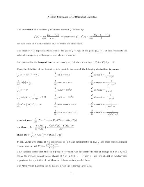
A <strong>Brief</strong> <strong>Summary</strong> <strong>of</strong> <strong>Differential</strong> <strong>Calculus</strong><br />
<strong>The</strong> derivative <strong>of</strong> a function f is another function f ′ defined by<br />
f ′ f(v) − f(x)<br />
(x) = lim<br />
v→x v − x<br />
for each value <strong>of</strong> x in the domain <strong>of</strong> f for which the limit exists.<br />
or (equivalently) f ′ f(x + h) − f(x)<br />
(x) = lim<br />
h→0 h<br />
<strong>The</strong> number f ′ (c) represents the slope <strong>of</strong> the graph y = f(x) at the point (c, f(c)). It also represents the<br />
rate <strong>of</strong> change <strong>of</strong> y with respect to x when x is near c.<br />
An equation for the tangent line to the curve y = f(x) when x = c is y − f(c) = f ′ (c)(x − c).<br />
Using the definition <strong>of</strong> the derivative, it is possible to establish the following derivative formulas.<br />
d<br />
dx xr = rx r−1 , r = 0<br />
d<br />
dx<br />
ln |x| = 1<br />
x<br />
d<br />
dx ex = e x<br />
d<br />
dx log a |x| =<br />
1<br />
, a > 0<br />
(lna)x<br />
d<br />
dx ax = (lna)a x , a > 0<br />
product rule:<br />
quotient rule:<br />
chain rule:<br />
d<br />
dx<br />
d<br />
dx<br />
sin x = cosx<br />
cosx = − sin x<br />
d<br />
dx tan x = sec2 x<br />
d<br />
dx cotx = − csc2 x<br />
d<br />
dx<br />
d<br />
dx<br />
sec x = secxtan x<br />
csc x = − cscxcotx<br />
d ′ ′<br />
F(x)G(x) = F(x)G (x) + G(x)F (x)<br />
dx<br />
d<br />
dx<br />
<br />
F(x)<br />
<br />
=<br />
G(x)<br />
G(x)F ′ (x) − F(x)G ′ (x)<br />
(G(x)) 2<br />
d<br />
dx F G(x) = F ′ G(x) G ′ (x)<br />
d<br />
dx<br />
d<br />
dx<br />
d<br />
dx<br />
d<br />
dx<br />
d<br />
dx<br />
d<br />
dx<br />
arcsinx =<br />
1<br />
√ 1 − x 2<br />
1<br />
arccosx = − √<br />
1 − x2 arctanx = 1<br />
1 + x 2<br />
arccotx = − 1<br />
1 + x 2<br />
1<br />
arcsecx =<br />
|x| √ x2 − 1<br />
1<br />
arccscx = −<br />
|x| √ x2 − 1<br />
Mean Value <strong>The</strong>orem: If f is continuous on [a, b] and differentiable on (a, b), then there exists a number<br />
c in (a, b) such that f ′ f(b) − f(a)<br />
(c) = .<br />
b − a<br />
This theorem states that there is a point c for which the instantaneous rate <strong>of</strong> change <strong>of</strong> f at c (f ′ (c))<br />
equals the average (mean) rate <strong>of</strong> change <strong>of</strong> f on [a, b] ((f(b) − f(a))/(b − a)). You should be familiar with<br />
a graphical interpretation <strong>of</strong> this theorem; it involves two parallel lines.<br />
<strong>The</strong> Mean Value <strong>The</strong>orem can be used to prove the following three facts.<br />
1
1. If f ′ is positive (negative) on an interval I, then f is increasing (decreasing) on I. This fact makes it<br />
possible to use f ′ to determine the values <strong>of</strong> x for which f has a relative maximum value or a relative<br />
minimum value. <strong>The</strong> first step is to find the critical points <strong>of</strong> f: points x in the domain <strong>of</strong> f for which<br />
either f ′ (x) = 0 or f ′ (x) does not exist. <strong>The</strong>n the First Derivative Test can be used to determine the<br />
nature <strong>of</strong> the critical point.<br />
2. If f ′′ is positive (negative) on an interval I, then f is concave up (concave down) on I. An inflection<br />
point occurs where the graph changes concavity. Possible inflection points occur when f ′′ (x) = 0, but it is<br />
necessary to check that the concavity actually changes at such points.<br />
3. If f ′ = g ′ on an interval I, then there is a constant C such that g(x) = f(x) + C for all x in I.<br />
A function f is continuous at a number c if lim<br />
x→c f(x) = f(c). This fact guarantees that the graph <strong>of</strong> f does<br />
not have a break at c. An important theorem states: If f is differentiable at c, then f is continuous at c.<br />
However, the converse is false; the function f(x) = |x| is continuous at 0 but not differentiable at 0.<br />
Intermediate Value <strong>The</strong>orem: If f is continuous on a closed interval [a, b] and v is any number between<br />
f(a) and f(b), then there is a number c in (a, b) such that f(c) = v.<br />
Extreme Value <strong>The</strong>orem: If f is continuous on a closed interval [a, b], then there exist numbers c and d<br />
in [a, b] such that f(c) ≤ f(x) ≤ f(d) for all x in [a, b]. (<strong>The</strong> number f(c) is the minimum value <strong>of</strong> f on [a, b]<br />
and the number f(d) is the maximum value <strong>of</strong> f on [a, b].)<br />
Definition <strong>of</strong> limit: Let f be defined on some open interval containing the point c, except possibly at<br />
c. <strong>The</strong>n lim<br />
x→c f(x) = L if for each ǫ > 0 there exists δ > 0 such that |f(x) − L| < ǫ for all x that satisfy<br />
0 < |x − c| < δ.<br />
A function f has a vertical asymptote x = c if either lim<br />
x→c− |f(x)| = ∞ or lim<br />
x→c +<br />
|f(x)| = ∞.<br />
A function f has a horizontal asymptote y = d if either lim<br />
x→∞<br />
f(x) = d or lim<br />
x→−∞<br />
f(x) = d.<br />
Various algebraic techniques (factoring, expanding, finding a common denominator, multiplying by the<br />
conjugate) can be used to evaluate limits. <strong>The</strong> following rule is sometimes useful for computing limits <strong>of</strong> the<br />
form 0/0 or ∞/∞; these are known as indeterminate forms. <strong>The</strong> suitable conditions mentioned in the<br />
hypotheses involve continuity and differentiability conditions that will always be met by the functions we<br />
encounter.<br />
L’Hôpital’s Rule: Under suitable conditions on the functions f and g, if either lim<br />
x→∗ f(x) = 0 = lim<br />
x→∗ g(x)<br />
f(x) f<br />
or lim f(x) = ∞ = lim g(x), then lim = lim<br />
x→∗ x→∗ x→∗ g(x) x→∗<br />
′ (x)<br />
g ′ , assuming that the latter limit exists. (<strong>The</strong> limits<br />
(x)<br />
here can be <strong>of</strong> any type; x → c, x → c + , x → c− , x → ∞, x → −∞.)<br />
2