Solving Delay Differential Equations - Radford University

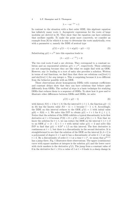
4 L.F. Shampine and S. Thompson
λ = −αe −λτ + 1
In contrast to the situation with a first order ODE, this algebraic equation
has infinitely many roots λ. Asymptotic expressions for the roots of large
modulus are derived in [9]. They show that the equation can have solutions
that oscillate rapidly. To make the point more concretely, we consider an
example from [9] for which it is easy to determine the roots analytically, even
with a parameter a, namely the DDE of neutral type
y ′ (t) = y ′ (t − τ) + a(y(t) − y(t − τ)) (5)
Substituting y(t) = e λt into this equation leads to
(λ − a)(1 − e −λτ ) = 0
The two real roots 0 and a are obvious. They correspond to a constant solution
and an exponential solution y(t) = e at , respectively. These solutions
are not surprising because they are like what we might find with an ODE.
However, any λτ leading to a root of unity also provides a solution. Written
in terms of real functions, we find then that there are solutions cos(2πnt/τ)
and sin(2πnt/τ) for any integer n. This is surprising because it is so different
from the behavior possible with an ODE.
These observations about homogeneous DDEs with constant coefficients
and constant delays show that they can have solutions that behave quite
differently from ODEs. The method of steps is a basic technique for studying
DDEs that reduces them to a sequence of ODEs. To show how it goes and to
illustrate other differences between ODEs and DDEs, we solve
y ′ (t) = y(t − 1) (6)
with history S(t) = 1 for t ≤ 0. On the interval 0 ≤ t ≤ 1, the function y(t−1)
in (6) has the known value S(t − 1) = 1 because t − 1 ≤ 0. Accordingly,
the DDE on this interval reduces to the ODE y ′ (t) = 1 with initial value
y(0) = S(0) = 1. We solve this IVP to obtain y(t) = t + 1 for 0 ≤ t ≤ 1.
Notice that the solution of the DDE exhibits a typical discontinuity in its first
derivative at t = 0 because S ′ (0) = 0 = y ′ (0−) and y ′ (0+) = 1. Now that we
know the solution for t ≤ 1, we can reduce the DDE on the interval 1 ≤ t ≤ 2
to an ODE y ′ = (t − 1) + 1 = t with initial value y(1) = 2 and solve this
IVP to find that y(t) = 0.5t 2 + 1.5 on this interval. The first derivative is
continuous at t = 1, but there is a discontinuity in the second derivative. It is
straightforward to see that the solution of the DDE on the interval [k, k +1] is
a polynomial of degree k + 1 and it has a discontinuity of order k + 1 at time
t = k. By a discontinuity of order k + 1 at a time t = t ∗ , we mean that y (k+1)
has a jump there. Fig. 1 illustrates these observations. The upper (continuous)
curve with square markers at integers is the solution y(t) and the lower curve
with circle markers is the derivative y ′ (t). The jump from a constant value of
0 in the derivative for t < 0 to a value of 1 at t = 0 leads to a sharp change in