Solving Delay Differential Equations - Radford University

Numerical Solution of Delay Differential 

Equations 

L.F. Shampine 1 and S. Thompson 2 

1 

Mathematics Department, Southern Methodist University, Dallas, TX 75275 

shampine@smu.edu 

2 

Dept. of Mathematics & Statistics, Radford University, Radford, VA 24142 

thompson@radford.edu 

Summary. After some introductory examples, this chapter considers some of the 

ways that delay differential equations (DDEs) differ from ordinary differential equations 

(ODEs). It then discusses numerical methods for DDEs and in particular, how 

the Runge–Kutta methods that are so popular for ODEs can be extended to DDEs. 

The treatment of these topics is complete, but it is necessarily brief, so it would 

be helpful to have some background in the theory of ODEs and their numerical 

solution. The chapter goes on to consider software issues special to the numerical 

solution of DDEs and concludes with some substantial numerical examples. Both 

topics are discussed in concrete terms using the programming languages Matlab 

and Fortran 90/95, so a familiarity with one or both languages would be helpful. 

Key words: DDEs, Propagated discontinuities, Vanishing delays, Numerical methods, 

Runge–Kutta, Continuous extension, Event location, Matlab, Fortran 90/95 

1 Introduction 

Ordinary differential equations (ODEs) have been used to model physical phenomena 

since the concept of differentiation was first developed and nowadays 

complicated ODE models can be solved numerically with a high degree of 

confidence. It was recognized early that phenomena may have a delayed effect 

in a differential equation, leading to what is called a delay differential equation 

(DDE). For instance, fishermen along the west coast of South America 

have long observed a sporadic and abrupt warming of the cold waters that 

support the food chain. The recent investigation [10] of this El-Niño/Southern 

Oscillation (ENSO) phenomenon discusses the history of models starting in 

the 1980s that account for delayed feedbacks. An early model of this kind, 

T ′ (t) = T (t) − αT (t − τ) (1) 

for constant α > 0, is simple enough to study analytically. It is the term 

involving a constant lag or delay τ > 0 in the independent variable that

2 L.F. Shampine and S. Thompson 

makes this a DDE. An obvious distinction between this DDE and an ODE is 

that specifying the initial value T (0) is not enough to determine the solution 

for t ≥ 0; it is necessary to specify the history T (t) for −τ ≤ t ≤ 0 for the 

differential equation even to be defined for 0 ≤ t ≤ τ. The paper [10] goes on 

to develop and study a more elaborate nonlinear model with periodic forcing 

and a number of physical parameters of the form 

h ′ (t) = −a tanh[κh(t − τ))] + b cos(2πωt) (2) 

These models exemplify DDEs with constant delays. The first mathematical 

software for solving DDEs is dmrode [17], which did not appear until 1975. 

Today a good many programs that can solve reliably first order systems of 

DDEs with constant delays are available, though the paper [10] makes clear 

that even for this relatively simple class of DDEs, there can be serious computational 

difficulties. This is not just a matter of developing software, rather 

that DDEs have more complex behavior than ODEs. Some numerical results 

for (2) are presented in §4.1. 

Some models have delays τj(t) that depend on time. Provided that the delays 

are bounded away from zero, the models behave similarly to those with 

constant delays and they can be solved with some confidence. However, if 

a delay goes to zero, the differential equation is said to be singular at that 

time. Such singular problems with vanishing delays present special difficulties 

in both theory and practice. As a concrete example of a problem with 

two time–dependent delays, we mention one that arises from delayed cellular 

neural networks [31]. The fact that the delays are sometimes very small and 

even vanish periodically during the integration makes this a relatively difficult 

problem. 

y ′ 1(t) = −6y1(t) + sin(2t)f(y1(t)) + cos(3t)f(y2(t)) 

 

 

1 + cos(t) 

+ sin(3t)f y1 t − + sin(t)f 

2 

+4 sin(t) 

y ′ 2(t) = −7y2(t) + cos(t) 

f(y1(t)) + 

3 

cos(2t) 

f(y2(t)) 

 

 

2 

 

1 + cos(t) 

+ cos(t)f y1 t − + cos(2t)f 

2 

+2 cos(t) 

y2 

y2 

 

t − 

 

t − 

 

1 + sin(t) 

2 

 

1 + sin(t) 

2 

Here f(x) = (|x + 1| − |x − 1|)/2. The problem is defined by this differential 

equation and the history y1(t) = −0.5 and y2(t) = 0.5 for t ≤ 0. A complication 

with this particular example is that there are time–dependent impulses, 

but we defer discussion of that issue to §4.3 where we solve it numerically 

as in [6]. Some models have delays that depend on the solution itself as well 

as time, τ(t, y). Not surprisingly, it is more difficult to solve such problems 

because only an approximation to the solution is available for defining the 

delays.

Numerical Solution of Delay Differential Equations 3 

Now that we have seen some concrete examples of DDEs, let us state more 

formally the equations that we discuss in this chapter. In a first order system 

of ODEs 

y ′ (t) = f(t, y(t)) (3) 

the derivative of the solution depends on the solution at the present time t. 

In a first order system of DDEs the derivative also depends on the solution at 

earlier times. As seen in the extensive bibliography [2], such problems arise in 

a wide variety of fields. In this chapter we consider DDEs of the form 

y ′ (t) = f(t, y(t), y(t − τ1), y(t − τ2), . . . , y(t − τk)) (4) 

Commonly the delays τj here are positive constants. There is, however, considerable 

and growing interest in systems with time–dependent delays τj(t) and 

systems with state–dependent delays τj(t, y(t)). Generally we suppose that 

the problem is non–singular in the sense that the delays are bounded below 

by a positive constant, τj ≥ τ > 0. We shall see that it is possible to adapt 

methods for the numerical solution of initial value problems (IVPs) for ODEs 

to the solution of initial value problems for DDEs. This is not straightforward 

because DDEs and ODEs differ in important ways. Equations of the form (4), 

even with time– and state–dependent delays, do not include all the problems 

that arise in practice. Notably absent are equations that involve a derivative 

with delayed argument like y ′ (t − τm) on the right hand side. Equations with 

such terms are said to be of neutral type. Though we comment on neutral 

equations in passing, we study in this chapter just DDEs of the form (4). We 

do this because neutral DDEs can have quite different behavior, behavior that 

is numerically challenging. Although we cite programs that have reasonable 

prospects for solving a neutral DDE, the numerical solution of neutral DDEs 

is still a research area. 

2 DDEs Are Not ODEs 

In this section we consider some of the most important differences between 

DDEs and ODEs. A fundamental technique for solving a system of DDEs 

is to reduce it to a sequence of ODEs. This technique and other important 

methods for solving DDEs are illustrated. 

The simple ENSO model (1) is a constant coefficient, homogeneous differential 

equation. If it were an ODE, we might solve it by looking for solutions of 

the form T (t) = e λt . Substituting this form into the ODE leads to an algebraic 

equation, the characteristic equation, for values λ that provide a solution. For 

a first order equation, there is only one such value. The same approach can 

be applied to DDEs. Here it leads first to 

λe λt = −αe λ(t−τ) + e λt 

and then to the characteristic equation


λ = −αe −λτ + 1 

In contrast to the situation with a first order ODE, this algebraic equation 

has infinitely many roots λ. Asymptotic expressions for the roots of large 

modulus are derived in [9]. They show that the equation can have solutions 

that oscillate rapidly. To make the point more concretely, we consider an 

example from [9] for which it is easy to determine the roots analytically, even 

with a parameter a, namely the DDE of neutral type 

y ′ (t) = y ′ (t − τ) + a(y(t) − y(t − τ)) (5) 

Substituting y(t) = e λt into this equation leads to 

(λ − a)(1 − e −λτ ) = 0 

The two real roots 0 and a are obvious. They correspond to a constant solution 

and an exponential solution y(t) = e at , respectively. These solutions 

are not surprising because they are like what we might find with an ODE. 

However, any λτ leading to a root of unity also provides a solution. Written 

in terms of real functions, we find then that there are solutions cos(2πnt/τ) 

and sin(2πnt/τ) for any integer n. This is surprising because it is so different 

from the behavior possible with an ODE. 

These observations about homogeneous DDEs with constant coefficients 

and constant delays show that they can have solutions that behave quite 

differently from ODEs. The method of steps is a basic technique for studying 

DDEs that reduces them to a sequence of ODEs. To show how it goes and to 

illustrate other differences between ODEs and DDEs, we solve 

y ′ (t) = y(t − 1) (6) 

with history S(t) = 1 for t ≤ 0. On the interval 0 ≤ t ≤ 1, the function y(t−1) 

in (6) has the known value S(t − 1) = 1 because t − 1 ≤ 0. Accordingly, 

the DDE on this interval reduces to the ODE y ′ (t) = 1 with initial value 

y(0) = S(0) = 1. We solve this IVP to obtain y(t) = t + 1 for 0 ≤ t ≤ 1. 

Notice that the solution of the DDE exhibits a typical discontinuity in its first 

derivative at t = 0 because S ′ (0) = 0 = y ′ (0−) and y ′ (0+) = 1. Now that we 

know the solution for t ≤ 1, we can reduce the DDE on the interval 1 ≤ t ≤ 2 

to an ODE y ′ = (t − 1) + 1 = t with initial value y(1) = 2 and solve this 

IVP to find that y(t) = 0.5t 2 + 1.5 on this interval. The first derivative is 

continuous at t = 1, but there is a discontinuity in the second derivative. It is 

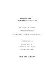
straightforward to see that the solution of the DDE on the interval [k, k +1] is 

a polynomial of degree k + 1 and it has a discontinuity of order k + 1 at time 

t = k. By a discontinuity of order k + 1 at a time t = t ∗ , we mean that y (k+1) 

has a jump there. Fig. 1 illustrates these observations. The upper (continuous) 

curve with square markers at integers is the solution y(t) and the lower curve 

with circle markers is the derivative y ′ (t). The jump from a constant value of 

0 in the derivative for t < 0 to a value of 1 at t = 0 leads to a sharp change in


the solution there. The discontinuity propagates to t = 1 where the derivative 

has a sharp change and the solution has a less obvious change in its concavity. 

The jump in the third derivative at t = 2 is not noticeable in the plot of y(t). 

6 

5 

4 

3 

2 

1 

0 

−1 −0.5 0 0.5 1 1.5 2 2.5 3 

Fig. 1. Solution Smoothing. 

In principle we can proceed in a similar way with the general equation (4) 

for delays that are bounded away from zero, τj ≥ τ > 0. With the history 

function S(t) defined for t ≤ t0, the DDEs reduce to ODEs on the interval 

[t0, t0 +τ] because for each j, the argument t−τj ≤ t−τ ≤ t0 and the y(t−τj) 

have the known values S(t − τj). Thus, we have an IVP for a system of ODEs 

with initial value y(t0) = S(t0). We solve this problem on [t0, t0 + τ] and 

extend the definition of S(t) to this interval by taking it to be the solution 

of this IVP. Now that we know the solution for t ≤ t0 + τ, we can move on 

to the interval [t0 + τ, t0 + 2τ], and so forth. In this way we can see that the 

DDEs have a unique solution on the whole interval of interest by solving a 

sequence of IVPs for ODEs. As with the simple example there is generally a 

discontinuity in the first derivative at the initial point. If a solution of (4) has 

a discontinuity at the time t ∗ of order k, then as the variable t moves through 

t ∗ + τj, there is a discontinuity in y (k+1) because of the term y(t − τj) in the 

DDEs. With multiple delays, a discontinuity at the time t ∗ is propagated to 

the times 

t ∗ + τ1, t ∗ + τ2, . . . , t ∗ + τk


and each of these discontinuities is in turn propagated. If there is a discontinuity 

at the time t ∗ of order k, the discontinuity at each of the times t ∗ + τj is 

of order at least k + 1, and so on. This is a fundamental distinction between 

DDEs and ODEs: There is normally a discontinuity in the first derivative at 

the initial point and it is propagated throughout the interval of interest. Fortunately, 

for problems of the form (4) the solution becomes smoother as the 

integration proceeds. That is not the case with neutral DDEs, which is one 

reason that they are so much more difficult. 

Neves and Feldstein [18] characterize the propagation of derivative discontinuities. 

The times at which discontinuities occur form a discontinuity tree. If 

there is a derivative discontinuity at T , the equation (4) shows that there will 

generally be a discontinuity in the derivative of one higher order if for some 

j, the argument t − τj(t, y(t)) = T because the term y(t − τj(t, y(t)) has a 

derivative discontinuity at T . Accordingly, the times at which discontinuities 

occur are zeros of functions 

t − τj(t, y(t)) − T = 0 (7) 

It is required that the zeros have odd multiplicity so that the delayed argument 

actually crosses the previous jump point and in practice, it is always 

assumed that the multiplicity is one. Although the statement in [18] is rather 

involved, the essence is that if the delays are bounded away from zero and 

delayed derivatives are not present, a derivative discontinuity is propagated 

to a discontinuity in (at least) the next higher derivative. On the other hand, 

smoothing does not necessarily occur for neutral problems nor for problems 

with vanishing delays. For constant and time–dependent delays, the discontinuity 

tree can be constructed in advance. If the delay depends on the state 

y, the points in the tree are located by solving the algebraic equations (7). A 

very important practical matter is that the solvers have to track only discontinuities 

with order lower than the order of the integration method because the 

behavior of the method is not affected directly by discontinuities in derivatives 

of higher order. 

Multiple delays cause special difficulties. Suppose, for example, that one 

delay is 1 and another is 0.001. A discontinuity in the first derivative at the 

initial point t = 0 propagates to 0.001, 0.002, 0.003, . . . because of the second 

delay. These “short” delays are troublesome, but the orders of the discontinuities 

increase and soon they do not trouble numerical methods. However, the 

other delay propagates the initial discontinuity to t = 1 and the discontinuity 

there is then propagated to 1.001, 1.002, 1.003, . . . because of the second delay. 

That is, the effects of the short delay die out, but they recur because of the 

longer delay. Another difficulty is that discontinuities can cluster. Suppose 

that one delay is 1 and another is 1/3. The second delay causes an initial discontinuity 

at t = 0 to propagate to 1/3, 2/3, 3/3, . . . and the first delay causes 

it to propagate to t = 1, . . .. In principle the discontinuity at 3/3 occurs at the 

same time as the one at 1, but 1/3 is not represented exactly in finite precision 

arithmetic, so it is found that in practice there are two discontinuities that


are extremely close together. This simple example is an extreme case, but it 

shows how innocuous delays can lead to clustering of discontinuities, clearly 

a difficult situation for numerical methods. 

There is no best way to solve DDEs and as a result, a variety of methods 

that have been used for ODEs have been modified for DDEs and implemented 

in modern software. It is possible, though awkward in some respects, to adapt 

linear multistep methods for DDEs. This approach is used in the snddelm 

solver [15] which is based on modified Adams methods [24]. There are a few 

solvers based on implicit Runge–Kutta methods. Several are described in [12, 

14, 25], including two codes, radar5 and ddesd, that are based on Radau IIA 

collocation methods. By far the most popular approach to non–stiff problems 

is to use explicit Runge–Kutta methods [3, 13]. Widely used solvers include 

archi [21, 22], dde23 [4, 29], ddverk [7, 8], and dde solver [5, 30]. Because the 

approach is so popular, it is the one that we discuss in this chapter. Despite 

sharing a common approach, the codes cited deal with important issues in 

quite different ways. 

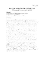
Before taking up numerical issues and how they are resolved, we illustrate 

the use of numerical methods by solving the model (1) over [0, 6] for α = 

2 and τ = 1 with two history functions, T (t) = 1 − t and T (t) = 1. By 

exploiting features of the language, the Matlab solvers dde23 and ddesd 

and the Fortran 90/95 solver dde solver make it nearly as easy to solve 

DDEs as ODEs. Because of this and because we are very familiar with them, 

we use these solvers for all our numerical examples. A program that solves 

the DDE (1) with both histories and plots the results is 

function Ex1 

lags = 1; tspan = [0 6]; 

sol1 = dde23(@dde,lags,@history,tspan); 

sol2 = dde23(@dde,lags,1,tspan); 

tplot = linspace(0,6,100); 

T1 = deval(sol1,tplot); 

T2 = deval(sol2,tplot); 

% Add linear histories to the plots: 

tplot = [-1 tplot]; T1 = [1 T1]; T2 = [2 T2]; 

plot(tplot,T1,tplot,T2,0,1,’o’) 

%--Subfunctions--------------------function 

dydt = dde(t,T,Z) 

dydt = T - 2*Z; 

function s = history(t) 

s = 1 - t; 

The output of this program is displayed as Fig. 2. Although Matlab displays 

the output in color, all the figures of this chapter are monochrome. Except 

for the additional information needed to define a delay differential equation, 

solving a DDE with constant delays using dde23 is nearly the same as solving 

an ODE with ode23. The first argument tells the solver of the function for


evaluating the DDEs (4). The lags argument is a vector of the lags τ1, . . . , τk. 

There is only one lag in the example DDE, so the argument is here a scalar. 

The argument tspan specifies the interval [t0, tf ] of interest. Unlike the ODE 

solvers of Matlab, the DDE solvers require that t0 < tf . The third argument 

is a function for evaluating the history, i.e., the solution for t ≤ t0. A 

constant history function is so common that the solver allows users to supply 

a constant vector instead of a function and that was done in computing the 

second solution. The first two arguments of the function for evaluating the 

DDEs is the same as for a system of ODEs, namely the independent variable 

t and a column vector of dependent variables approximating y(t). Here the 

latter is called T and is a scalar. A challenging task for the user interface is 

to accomodate multiple delays. This is done with the third argument Z which 

is an array of k columns. The first column approximates y(t − τ1) with τ1 

defined as the first delay in lag. The second column corresponds to the second 

delay, and so forth. Here there is only one delay and only one dependent 

variable, so Z is a scalar. A notable difference between dde23 and ode23 is 

the output, here called sol. The ODE solvers of Matlab optionally return 

solutions as a complex data structure called a structure, but that is the only 

form of output from the DDE solvers. The solution structure sol1 returned 

by the first integration contains the mesh that was selected as the field sol1.x 

and the solution at these points as the field sol1.y. With this information 

the first solution can be plotted by plot(sol1.x,sol1.y). Often this is satisfactory, 

but this particular problem is so easy that values of the solution 

at mesh points alone does not provide a smooth graph. Approximations to 

the solution can be obtained anywhere in the interval of interest by means of 

the auxiliary function deval. In the example program the two solutions are 

approximated at 100 equally spaced points for plotting. A marker is plotted 

at (0, T (0)) to distinguish the two histories from the corresponding computed 

solutions of (1). The discontinuity in the first derivative at the initial point is 

clear for the history T (t) = 1, but the discontinuity in the second derivative 

at t = 1 is scarcely visible. 

3 Numerical Methods and Software Issues 

The method of steps and modifications of methods for ODEs can be used 

to solve DDEs. Because they are so popular, we study in this chapter only 

explicit Runge–Kutta methods. In addition to discussing basic algorithms, we 

take up important issues that arise in designing software for DDEs. 

3.1 Explicit Runge–Kutta Methods 

Given yn ≈ y(tn), an explicit Runge–Kutta method for a first order system 

of ODEs (3) takes a step of size hn to form yn+1 ≈ y(tn+1) at tn+1 = tn + hn 

as follows. It first evaluates the ODEs at the beginning of the step,

25 

20 

15 

10 

5 

0 

−5 


−10 

−1 0 1 2 3 4 5 6 

Fig. 2. The Simple ENSO Model (1) for Two Histories. 

and then for j = 2, 3, . . . , s forms 

It finishes with 

yn,j = yn + hn 

yn,1 = yn, fn,1 = f(tn, yn,1) 

j−1 

βj,kfn,k, fn,j = f(tn + αjhn, yn,j) 

k=1 

yn+1 = yn + hn 

s 

k=1 

γkfn,k 

The constants s, βj,k, αj, and γk are chosen to make yn+1 an accurate approximation 

to y(tn+1). The numerical integration of a system of ODEs starts 

with given initial values y0 = y(t0) and then forms a sequence of approximations 

y0, y1, y2, . . . to the solution at times t0, t1, t2, . . . that span the interval 

of interest, [t0, tf ]. For some purposes it is important to approximate the solution 

at times t that are not in the mesh when solving a system of ODEs, 

but this is crucial to the solution of DDEs. One of the most significant developments 

in the theory and practice of Runge–Kutta methods is a way to 

approximate the solution accurately and inexpensively throughout the span 

of a step, i.e., anywhere in [tn, tn+1]. This is done with a companion formula 

called a continuous extension. 

A natural and effective way to solve DDEs can be based on an explicit 

Runge–Kutta method and the method of steps. The first difficulty is that in


taking a step, the function f must be evaluated at times tn + αjhn, which 

for the delayed arguments means that we need values of the solution at times 

(tn + αjhn) − τm which may be prior to tn. Generally these times do not coincide 

with mesh points, so we obtain the solution values from an interpolant. 

For this purpose linear multistep methods are attractive because the popular 

methods all have natural interpolants that provide accurate approximate 

solutions between mesh points. For other kinds of methods it is natural to 

use Hermite interpolation for this purpose. However, though formally correct 

as the step size goes to zero, the approach does not work well with Runge– 

Kutta methods. That is because these methods go to considerable expense 

to form an accurate approximation at the end of the step and as a corollary, 

an efficient step size is often too large for accurate results from direct interpolation 

of solution and first derivative at several previous steps. Nowadays 

codes based on Runge–Kutta formulas use a continuous extension of the basic 

formula that supplements the function evaluations formed in taking the step 

to obtain accurate approximations throughout [tn, tn+1]. This approach uses 

only data from the current interval. With any of these approaches we obtain a 

polynomial interpolant that approximates the solution over the span of a step 

and in aggregate, the interpolants form a piecewise–polynomial function that 

approximates y(t) from t0 to the current tn. Care must be taken to ensure 

that the accuracy of the interpolant reflects that of the basic formula and 

that various polynomials connect at mesh points in a sufficiently smooth way. 

Details can be found in [3] and [13]. It is important to appreciate that interpolation 

is used for other purposes, too. We have already seen it used to get 

the smooth graph of Fig. 2. It is all but essential when solving (7). Capable 

solvers also use interpolation for event location, a matter that we discuss in 

§3.3. 

Short delays arise naturally and as we saw by example in §1, it may even 

happen that a delay vanishes. If no delayed argument occurs prior to the 

initial point, the DDE has no history, so it is called an initial value DDE. 

A simple example is y ′ (t) = y(t 2 ) for t ≥ 0. A delay that vanishes can lead 

to quite different behavior—the solution may not extend beyond the singular 

point or it may extend, but not be unique. Even when the delays are all 

constant, “short” delays pose an important practical difficulty: Discontinuities 

smooth out as the integration progresses, so we may be able to use a step size 

much longer than a delay. In this situation an explicit Runge–Kutta formula 

needs values of the solution at “delayed” arguments that are in the span 

of the current step. That is, we need an approximate solution at points in 

[tn, tn+1] before yn+1 has been computed. Early codes simply restrict the 

step size so as to avoid this difficulty. However, the most capable solvers 

predict a solution throughout [tn, tn+1] using the continuous extension from 

the preceding step. They compute a tentative yn+1 using predicted values 

for the solution at delayed arguments and then repeat using a continuous 

extension for the current step until the values for yn+1 converge. This is a 

rather interesting difference between ODEs and DDEs: If the step size is bigger


than a delay, a Runge–Kutta method that is explicit for ODEs is generally 

an implicit formula for yn+1 for DDEs. The iterative scheme for taking a 

step resembles a predictor–corrector iteration for evaluating an implicit linear 

multistep method. More details are available in [1, 29]. 

The order of accuracy of a Runge–Kutta formula depends on the smoothness 

of the solution in the span of the step. This is not usually a problem 

with ODEs, but we have seen that discontinuities are to be expected when 

solving DDEs. To maintain the order of the formula, we have to locate and 

step to discontinuities. The popular codes handle propagated discontinuities 

in very different ways. The solver dde23 allows only constant delays, so before 

starting the integration, it determines all the discontinuities in the interval of 

interest and arranges for these points to be included in the mesh t0, t1, . . .. 

Something similar can be done if the delays are time–dependent, but this is 

awkward, especially if there are many delays. The approach is not applicable 

to problems with state–dependent delays. For problems of this generality, 

discontinuities are located by solving (7) as the integration proceeds. If the 

function (7) changes sign between tn and tn+1, the algebraic equation is solved 

for the location of the discontinuity with the polynomial interpolant for this 

step, P (t), replacing y(t) in (7). After locating the first time t ∗ at which 

α(t ∗ , P (t ∗ )) − T = 0, the step to tn+1 is rejected and a shorter step is taken 

from tn to a new tn+1 = t ∗ . This is what dde solver does for general delays, 

but it uses the more efficient approach of building the discontinuity tree in 

advance for problems with constant delays. archi also solves (7), but tracking 

discontinuities is an option in this solver. ddverk does not track discontinuities 

explicitly, rather it uses the defect or residual of the solution to detect discontinuities. 

The residual r(t) of an approximate solution S(t) is the amount 

by which it fails to satisfy the differential equation: 

S ′ (t) = f(t, S(t), S(t − τ1), S(t − τ2), . . . , S(t − τk)) + r(t) 

On discovering a discontinuity, ddverk steps across with special interpolants. 

ddesd does not track propagated discontinuities. Instead it controls the residual, 

which is less sensitive to the effects of propagated discontinuities. radar5 

treats the step size as a parameter in order to locate discontinuities detected 

by error test failures; details are found in [11]. 

When solving a system of DDEs, it is generally necessary to supply an initial 

history function to provide solution values for t ≤ t0. Of course the history 

function must provide values for t as far back from t0 as the maximum delay. 

This is straightforward, but some DDEs have discontinuities at times prior to 

the initial point or even at the initial point. A few solvers, including dde23, 

ddesd, and dde solver, provide for this, but most codes do not because it 

complicates both the user interface and the program.


3.2 Error Estimation and Control 

Several quite distinct approaches to the vital issue of error estimation and 

control are seen in popular solvers. In fact, this issue most closely delineates 

the differences between DDE solvers. Popular codes like archi, dde23, 

dde solver, and ddverk use pairs of formulas for this purpose. The basic idea 

is to take each step with two formulas and estimate the error in the lower order 

result by comparison. The cost is kept down by embedding one formula in the 

other, meaning that one formula uses only fn,k that were formed in evaluating 

the other formula or at most a few extra function evaluations. The error of 

the lower order formula is estimated and controlled, but it is believed that the 

higher order formula is more accurate, so most codes advance the integration 

with the higher order result. This is called local extrapolation. In some ways an 

embedded pair of Runge–Kutta methods is rather like a predictor–corrector 

pair of linear multistep methods. 

If the pair is carefully matched, an efficient and reliable estimate of the 

error is obtained when solving a problem with a smooth solution. Indeed, 

most ODE codes rely on the robustness of the error estimate and step size 

selection procedures to handle derivative discontinuities. Codes that provide 

for event location and those based on control of the defect (residual) further 

improve the ability of a code to detect and resolve discontinuities. Because 

discontinuities in low–order derivatives are almost always present when solving 

DDEs, the error estimates are sometimes questionable. This is true even if a 

code goes to great pains to avoid stepping across discontinuities. For instance, 

ddverk monitors repeated step failures to discern whether the error estimate 

is not behaving as it ought for a smooth solution. If it finds a discontinuity in 

this way, it uses special interpolants to get past the discontinuity. The solver 

generally handles discontinuities quite well since the defect does a good job 

of reflecting discontinuities. Similarly, radar5 monitors error test failures to 

detect discontinuities and then treats the step size as a parameter to locate the 

discontinuity. Despite these precautions, the codes may still use questionable 

estimates near discontinuities. The ddesd solver takes a different approach. It 

exploits relationships between the residual and the error to obtain a plausible 

estimate of the error even when discontinuities are present; details may be 

found in [25]. 

3.3 Event Location 

Just as with ODEs it is often important to find out when something happens. 

For instance, we may need to find the first time a solution component attains 

a prescribed value because the problem changes then. Mathematically this is 

formulated as finding a time t ∗ for which one of a collection of functions 

g1(t, y(t)), g2(t, y(t)), . . . , gk(t, y(t))


vanishes. We say that an event occurs at time t ∗ and the task is called event 

location [28]. As with locating discontinuities, the idea is to monitor the event 

functions for a change of sign between tn and tn+1. When a change is encountered 

in, say, equation m, the algebraic equation gm(t, P (t)) = 0 is solved for 

t ∗ . Here P (t) is the polynomial continuous extension that approximates y(t) 

on [tn, tn+1]. Event location is a valuable capability that we illustrate with a 

substantial example in §4. A few remarks about this example will illustrate 

some aspects of the task. A system of two differential equations is used to 

model a two-wheeled suitcase that may wobble from one wheel to the other. 

If the event y1(t) − π/2 = 0 occurs, the suitcase has fallen over and the computation 

comes to an end. If the event y1(t) = 0 occurs, a wheel has hit the 

floor. In this situation we stop integrating and restart with initial conditions 

that account for the wheel bouncing. As this example makes clear, if there 

are events at all, we must find the first one if we are to model the physical 

situation properly. For both these event functions the integration is to terminate 

at an event, but it is common that we want to know when an event 

occurs and the value of the solution at that time, but we want the integration 

to continue. A practical difficulty is illustrated by the event of a wheel 

bouncing—the integration is to restart with y1(t) = 0, a terminal event! In 

the example we deal with this by using another capability, namely that we 

can tell the solver that we are interested only in events for which the function 

decreases through zero or increases through zero, or it does not matter how 

the function changes sign. Most DDE codes do not provide for event location. 

Among the codes that do are dde23, ddesd, and dde solver. 

3.4 Software Issues 

A code needs values from the past, so it must use either a fixed mesh that 

matches the delays or some kind of continuous extension. The former approach, 

used in early codes, is impractical or impossible for most DDEs. Modern 

codes adopt the latter approach. Using some kind of interpolation, they 

evaluate the solution at delayed arguments, but this requires that they store 

all the information needed for the interpolation. This information is saved in 

a solution history queue. The older Fortran codes had available only static 

storage and using a static queue poses significant complications. Since the 

size of the queue is not known in advance, users must either allocate excessively 

large queues or live with the fact that the code will be unsuccessful for 

problems when the queue fills. The difficulty may be avoided to some extent 

by using circular queues in which the oldest solution is replaced by new information 

when necessary. Of course this approach fails if discarded information 

is needed later. The dynamic storage available in modern programming languages 

like Matlab and Fortran 90/95 is vital to modern programs for the 

solution of DDEs. The dde23, ddesd, and dde solver codes use dynamic 

memory allocation to make the management of the solution queue transparent 

to the user and to allow the solution queue to be used on return from


the solver. Each of the codes trims the solution queue to the amount actually 

used at the end of the integration. The latest version of dde solver has an 

option for trimming the solution queue during the integration while allowing 

the user to save the information conveniently if desired. 

The more complex data structures available in modern languages are very 

helpful. The one used in the DDE solvers of Matlab is called a structure 

and the equivalent in Fortran 90/95 is called a derived type. By encapsulating 

all information about the solution in a structure, the user is relieved of the 

details about how some things are accomplished. An example is evaluation of 

the solution anywhere in the interval of interest. The mesh and the details 

of how the solution is interpolated are unobtrusive when stored in a solution 

structure. A single function deval is used to evaluate the solution computed 

by any of the differential equation solvers of Matlab. If the solution structure 

is called sol, there is a field, sol.solver, that is the name of the solver as a 

string, e.g., ’dde23’. With this deval knows how the data for the interpolant 

is stored and how to evaluate it. There are, in fact, a good many possibilities. 

For example, the ODE solvers that are based on linear multistep methods vary 

the order of the formula used from step to step, so stored in the structure 

is the order of the polynomial and the data defining it for each [tn, tn+1]. 

All the interpolants found in deval are polynomials, but several different 

representations are used because they are more natural to the various solvers. 

By encapsulating this information in a structure, the user need give no thought 

to the matter. A real dividend for libraries is that it is easy to add another 

solver to the collection. 

The event location capability discussed in §3.3 requires output in addition 

to the solution itself, viz., the location of events, which event function led 

to each event reported, and the solution at each event. It is difficult to deal 

properly with event location without modern language capabilities because the 

number of events is not known in advance. In the ODE solvers of Matlab 

this information is available in output arguments since the language provides 

for optional output arguments. Still, it is convenient to return the information 

as fields in a solution structure since a user may want to view only some of the 

fields. The equivalent in Fortran 90/95 is to return the solution as a derived 

type. This is especially convenient because the language does not provide for 

optional output. The example of §4.2 illustrates what a user interface might 

look like in both languages. 

In the numerical example of §4.2, the solver returns after an event, changes 

the solution, and continues the integration. This is easy with an ODE because 

continuation can be treated as a new problem. Not so with DDEs because they 

need a history. Output as a structure is crucial to a convenient implementation 

of this capability. To continue an integration, the solver is called with 

the output structure from the prior integration instead of the usual history 

function or vector. The computation proceeds as usual, but approximate solutions 

at delayed arguments prior to the starting point are taken from the 

previously computed solution. If the delays depend on time and/or state, they


might extend as far back as the initial data. This means that we must save 

the information needed to interpolate the solution from the initial point on. 

Indeed, the delays might be sufficiently long that values are taken from the 

history function or vector supplied for the first integration of the problem. 

This means that the history function or vector, as the case may be, must be 

held as a field in the solution structure for this purpose. A characteristic of 

the data structure is that fields do not have to be of the same type or size. 

Indeed, we have mentioned a field that is a string, fields that are arrays of 

length not known in advance, and a field that is a function handle. 

4 Examples 

Several collections of test problems are available to assess how well a particular 

DDE solver handles the issues and tasks described above. Each of the 

references [5, 7, 11, 19, 20, 25, 27, 29] describes a variety of test problems. 

In this section the two problems of §1 are solved numerically to show that a 

modern DDE solver may be used to investigate complex problems. With such 

a solver, it is not much more difficult to solve a first order system of DDEs 

than ODEs. Indeed, a design goal of the dde23, ddesd, and dde solver codes 

was to exploit capabilities in Matlab and Fortran 90/95 to make them as 

easy as possible to use, despite exceptional capabilities. We also supplement 

the discussion of event location in §3.3 with an example. Although it is easy 

enough to solve the DDEs, the problem changes at events and dealing with 

this is somewhat involved. We provide programs in both Matlab and Fortran 

90/95 that show even complex tasks can be solved conveniently with codes like 

dde23 and dde solver. Differences in the design of these codes are illustrated 

by this example. Further examples of the numerical solution of DDEs can be 

found in the documentation for the codes cited throughout the chapter. They 

can also can be found in a number of the references cited and in particular, 

the references of §6. 

4.1 El-Niño Southern Oscillation Variability Model 

Equation (2) is a DDE from [10] that models the El-Niño Southern Oscillation 

(ENSO) variability. It combines two key mechanisms that participate in ENSO 

dynamics, delayed negative feedback and seasonal forcing. They suffice to 

generate very rich behavior that illustrates several important features of more 

detailed models and observational data sets. In [10] a stability analysis of the 

model is performed in a three–dimensional space of its strength of seasonal 

forcing b, atmosphere–ocean coupling κ, and propagation period τ of oceanic 

waves across the Tropical Pacific. The physical parameters a, κ, τ, b, and ω are 

all real and positive. 

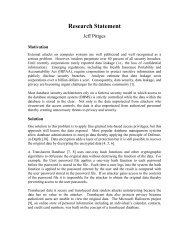
Fig. 3 depicts typical solutions computed with dde solver and constant 

history h(t) = 1 for t ≤ 0. It shows six solutions obtained by fixing b = 1, κ =


f 

e 

d 

c 

b 

a 

0 1 2 3 4 5 6 7 8 9 10 

Time 

Fig. 3. Examples of DDE model solutions. Model parameters are κ = 100 and 

b = 1, while τ increases from curve (a) to curve (f) as follows: (a) τ = 0.01, (b) 

τ = 0.025, (c) τ = 0.15, (d) τ = 0.45, (e) τ = 0.995, and (f) τ = 1. 

100 and varying the delay τ over two orders of magnitude, from τ = 10 −2 to 

τ = 1, with τ increasing from bottom to top in the figure. The sequence of 

changes in solution type as τ increases seen in this figure is typical for any 

choice of (b, κ). 

For a small delay, τ < π/(2 κ), we have a periodic solution with period 1 

(curve a); here the internal oscillator is completely dominated by the seasonal 

forcing. When the delay increases, the effect of the internal oscillator becomes 

visible: small wiggles, in the form of amplitude–modulated oscillations with a 

period of 4 τ, emerge as the trajectory crosses the zero line. However, these 

wiggles do not affect the overall period, which is still 1. The wiggle amplitude 

grows with τ (curve b) and eventually wins over the seasonal oscillations, resulting 

in period doubling (curve c). Further increase of τ results in the model 

passing through a sequence of bifurcations that produce solution behavior of 

considerable interest for understanding ENSO variability. 

Although solution of this DDE is straightforward with a modern solver, it is 

quite demanding for some parameters. For this reason the compiled computation 

of the Fortran dde solver was much more appropriate for the numerical 

study of [10] than the interpreted computation of the Matlab dde23. The 

curves in Fig. 3 provide an indication of how much the behavior of the solution 

depends on the delay τ. Further investigation of the solution behavior for 

different values of the other problem parameters requires the solution over extremely 

long intervals. The intervals are so long that it is impractical to retain 

all the information needed to evaluate an approximate solution anywhere in


the interval. These problems led to the option of trimming the solution queue 

in dde solver. 

4.2 Rocking Suitcase 

To illustrate event location for a DDE, we consider the following example 

from [26]. A two–wheeled suitcase may begin to rock from side to side as it 

is pulled. When this happens, the person pulling it attempts to return it to 

the vertical by applying a restoring moment to the handle. There is a delay 

in this response that can affect significantly the stability of the motion. This 

may be modeled with the DDE 

θ ′′ (t) + sign(θ(t))γ cos(θ(t)) − sin(θ(t)) + βθ(t − τ) = A sin(Ωt + η) 

where θ(t) is the angle of the suitcase to the vertical. This equation is solved 

on the interval [0, 12] as a pair of first order equations with y1(t) = θ(t) and 

y2(t) = θ ′ (t). Parameter values of interest are 

 

γ 

 

γ = 2.48, β = 1, τ = 0.1, A = 0.75, Ω = 1.37, η = arcsin 

A 

and the initial history is the constant vector zero. A wheel hits the ground (the 

suitcase is vertical) when y1(t) = 0. The integration is then to be restarted 

with y1(t) = 0 and y2(t) multiplied by the coefficient of restitution, here chosen 

to be 0.913. The suitcase is considered to have fallen over when |y1(t)| = π 

2 

and the run is then terminated. This problem is solved using dde23 with the 

following Matlab program. 

function sol = suitcase 

state = +1; 

opts = ddeset(’RelTol’,1e-5,’Events’,@events); 

sol = dde23(@ddes,0.1,[0; 0],[0 12],opts,state); 

ref = [4.516757065, 9.751053145, 11.670393497]; 

fprintf(’Kind of Event: dde23 reference\n’); 

event = 0; 

while sol.x(end) < 12 

event = event + 1; 

if sol.ie(end) == 1 

fprintf(’A wheel hit the ground. %10.4f %10.6f\n’,... 

sol.x(end),ref(event)); 

state = - state; 

opts = ddeset(opts,’InitialY’,[ 0; 0.913*sol.y(2,end)]); 

sol = dde23(@ddes,0.1,sol,[sol.x(end) 12],opts,state); 

else 

fprintf(’The suitcase fell over. %10.4f %10.6f\n’,... 

sol.x(end),ref(event));


break; 

end 

end 

plot(sol.y(1,:),sol.y(2,:)) 

xlabel(’\theta(t)’) 

ylabel(’\theta’’(t)’) 

%=========================================================== 

function dydt = ddes(t,y,Z,state) 

gamma = 0.248; beta = 1; A = 0.75; omega = 1.37; 

ylag = Z(1,1); 

dydt = [y(2); 0]; 

dydt(2) = sin(y(1)) - state*gamma*cos(y(1)) - beta*ylag ... 

+ A*sin(omega*t + asin(gamma/A)); 

function [value,isterminal,direction] = events(t,y,Z,state) 

value = [y(1); abs(y(1))-pi/2]; 

isterminal = [1; 1]; 

direction = [-state; 0]; 

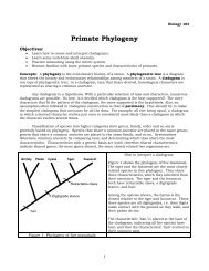
The program produces the phase plane plot depicted in Fig. 4. It also reports 

what kind of event occurred and the location of the event. The reference values 

displayed were computed with the dde solver code and much more stringent 

tolerances. 

Kind of Event: dde23 reference 

A wheel hit the ground. 4.5168 4.516757 

A wheel hit the ground. 9.7511 9.751053 

The suitcase fell over. 11.6704 11.670393 

This is a relatively complicated model, so we will elaborate on some aspects 

of the program. Coding of the DDE is straightforward except for evaluating 

properly the discontinuous coefficient sign(y1(t)). This is accomplished by 

initializing a parameter state to +1 and changing its sign whenever dde23 

returns because y1(t) vanished. Handling state in this manner ensures that 

dde23 does not need to deal with the discontinuities it would otherwise see if 

the derivative were coded in a manner that allowed state to change before 

the integration is restarted; see [28] for a discussion of this issue. After a call 

to dde23 we must consider why it has returned. One possibility is that it has 

reached the end of the interval of integration, as indicated by the last point 

reached, sol.x(end), being equal to 12. Another is that the suitcase has 

fallen over, as indicated by sol.ie(end) being equal to 2. Both cases cause 

termination of the run. More interesting is a return because a wheel hit the 

ground, y1(t) = 0, which is indicated by sol.ie(end) being equal to 1. The 

sign of state is then changed and the integration restarted. Because the wheel 

bounces, the solution at the end of the current integration, sol.y(:,end),

θ’(t) 

1 

0.5 

0 

−0.5 

−1 


−1.5 

−1 −0.5 0 0.5 

θ(t) 

1 1.5 2 

Fig. 4. Two–Wheeled Suitcase Problem. 

must be modified for use as initial value of the next integration. The InitialY 

option is used to deal with an initial value that is different from the history. 

The event y1(t) = 0 that terminates one integration occurs at the initial point 

of the next integration. As with the Matlab IVP solvers, dde23 does not 

terminate the run in this special situation of an event at the initial point. No 

special action is necessary, but the solver does locate and report an event at 

the initial point, so it is better practice to avoid this by defining more carefully 

the event function. When the indicator state is +1, respectively −1, we are 

interested in locating where the solution component y1(t) vanishes only if it 

decreases, respectively increases, through zero. We inform the solver of this by 

setting the first component of the argument direction to -state. Notice that 

ddeset is used to alter an existing options structure in the while loop. This 

is a convenient capability also present in odeset, the corresponding function 

for IVPs. The rest of the program is just a matter of reporting the results of 

the computations. Default tolerances give an acceptable solution, though the 

phase plane plot would benefit from plotting more solution values. Reducing 

the relative error tolerance to 1e-5 gives better agreement with the reference 

values. 

It is instructive to compare solving the problem with dde23 to solving it 

with dde solver. In contrast to the numerical study of the ENSO model, 

solving this problem is inexpensive in either computing environment, so the 

rather simpler program of the Matlab program outweighs the advantage in 

speed of the Fortran program.


We begin by contrasting briefly the user interface of the solvers. A simple 

problem is solved simply by defining it with a call like 

SOL = DDE_SOLVER(NVAR,DDES,BETA,HISTORY,TSPAN) (8) 

Here NVAR is an integer array of two entries or three entries. The first is 

NEQN, the number of DDEs, the second is NLAGS, the number of delays, 

the third, if present, is NEF, the number of event functions. DDES is the 

name of a subroutine for evaluating the DDEs. It has the form 

SUBROUTINE DDES(T,Y,Z,DY) (9) 

The input arguments are the independent variable T, a vector Y of NEQN 

components approximating y(T ), and an array Z that is NEQN × NLAGS. 

Column j of this array is an approximation to y(βj(T, y(T ))). The subroutine 

evaluates the DDEs with these arguments and returns y ′ (T ) as the vector DY 

of NEQN components. 

BETA is the name of a subroutine for evaluating the delays and HISTORY 

is the name of a subroutine for evaluating the initial history function. More 

precisely, the functions are defined by subroutines for general problems, but 

they are defined in a simpler way in the very common situations of constant 

lags and/or constant history. dde solver returns the numerical solution in the 

output structure SOL. The input vector TSPAN is used to inform the solver 

of the interval of integration and where approximate solutions are desired. 

TSPAN has at least two entries. The first entry is the initial point of the 

integration, t0, and the last is the final point, tf . If TSPAN has only two 

entries, approximate solutions are returned at all the mesh points selected by 

the solver itself. These points generally produce a smooth graph when the 

numerical solution is plotted. If TSPAN has entries t0 < t1 < . . . < tf , the 

solver returns approximate solutions at (only) these points. 

The call list of (8) resembles closely that of dde23. The design provides for 

a considerable variety of additional capabilities. This is accomplished in two 

ways. F90 provides for optional arguments that can be supplied in any order 

if associated with a keyword. This is used, for example, to pass to the solver 

the name of a subroutine EF for evaluating event functions and the name of a 

subroutine CHNG in which necessary problem changes are made when event 

times are located, with a call like 

SOL = DDE_SOLVER(NVAR, DDES, BETA, HISTORY, TSPAN, & 

EVENT_FCN=EF, CHANGE_FCN=CHNG) 

This ability is precisely what is needed to solve this problem. EF is used to 

define the residuals g1 = y1 and g2 = |y1| − π 

2 . CHNG is used to apply the 

coefficient of restitution and handle the STATE flag as in the solution for 

dde23. One of the optional arguments is a structure containing options. This 

structure is formed by a function called DDE SET that is analogous to the 

function ddeset used by dde23 (and ddesd). The call list of (8) uses defaults


for important quantities such as error tolerances, but of course, the user has 

the option of specifying quantities appropriate to the problem at hand. A more 

detailed discussion of these and other design issues may be found in [30]. Here 

is a Fortran 90 program that uses dde solver to solve this problem. 

MODULE define_DDEs 

IMPLICIT NONE 

INTEGER, PARAMETER :: NEQN=2, NLAGS=1, NEF=2 

INTEGER :: STATE 

CONTAINS 

SUBROUTINE DDES(T, Y, Z, DY) 

DOUBLE PRECISION :: T 

DOUBLE PRECISION, DIMENSION(NEQN) :: Y, DY 

DOUBLE PRECISION :: YLAG 

DOUBLE PRECISION, DIMENSION(NEQN,NLAGS) :: Z 

! Physical parameters 

DOUBLE PRECISION, PARAMETER :: gamma=0.248D0, beta=1D0, & 

A=0.75D0, omega=1.37D0 

YLAG = Z(1,1) 

DY(1) = Y(2) 

DY(2) = SIN(Y(1)) - STATE*gamma*COS(Y(1)) - beta*YLAG & 

+ A*SIN(omega*T + ASIN(gamma/A)) 

RETURN 

END SUBROUTINE DDES 

SUBROUTINE EF(T, Y, DY, Z, G) 

DOUBLE PRECISION :: T 

DOUBLE PRECISION, DIMENSION(NEQN) :: Y, DY 

DOUBLE PRECISION, DIMENSION(NEQN,NLAGS) :: Z 

DOUBLE PRECISION, DIMENSION(NEF) :: G 

G = (/ Y(1), ABS(Y(1)) - ASIN(1D0) /) 

RETURN 

END SUBROUTINE EF 

SUBROUTINE CHNG(NEVENT, TEVENT, YEVENT, DYEVENT, HINIT, & 

DIRECTION, ISTERMINAL, QUIT) 

INTEGER :: NEVENT 

INTEGER, DIMENSION(NEF) :: DIRECTION 

DOUBLE PRECISION :: TEVENT, HINIT 

DOUBLE PRECISION, DIMENSION(NEQN) :: YEVENT, DYEVENT 

LOGICAL :: QUIT 

LOGICAL, DIMENSION(NEF) :: ISTERMINAL


INTENT(IN) :: NEVENT,TEVENT 

INTENT(INOUT) :: YEVENT, DYEVENT, HINIT, DIRECTION, & 

ISTERMINAL, QUIT 

IF (NEVENT == 1) THEN 

! Restart the integration with initial values 

! that correspond to a bounce of the suitcase. 

STATE = -STATE 

YEVENT(1) = 0.0D0 

YEVENT(2) = 0.913*YEVENT(2) 

DIRECTION(1) = - DIRECTION(1) 

! ELSE 

! Note: 

! The suitcase fell over, NEVENT = 2. The integration 

! could be terminated by QUIT = .TRUE., but this 

! event is already a terminal event. 

ENDIF 

RETURN 

END SUBROUTINE CHNG 

END MODULE define_DDEs 

!********************************************************** 

PROGRAM suitcase 

! The DDE is defined in the module define_DDEs. The problem 

! is solved here with ddd_solver and its output written to 

! a file. The auxilary function suitcase.m imports the data 

! into Matlab and plots it. 

USE define_DDEs 

USE DDE_SOLVER_M 

IMPLICIT NONE 

! The quantities 

! NEQN = number of equations 

! NLAGS = number of delays 

! NEF = number of event functions 

! are defined in the module define_DDEs as PARAMETERs so 

! they can be used for dimensioning arrays here. They 

! pre assed to the solver in the array NVAR. 

INTEGER, DIMENSION(3) :: NVAR = (/NEQN,NLAGS,NEF/) 

TYPE(DDE_SOL) :: SOL


! The fields of SOL are expressed in terms of the 

! number of differential equations, NEQN, and the 

! number of output points, NPTS: 

! SOL%NPTS -- NPTS,number of output points. 

! SOL%T(NPTS) -- values of independent variable, T. 

! SOL%Y(NPTS,NEQN) -- values of dependent variable, Y, 

! corresponding to values of SOL%T. 

! When there is an event function, there are fields 

! SOL%NE -- NE, number of events. 

! SOL%TE(NE) -- locations of events 

! SOL%YE(NE,NEQN) -- values of solution at events 

! SOL%IE(NE) -- identifies which event occurred 

TYPE(DDE_OPTS) :: OPTS 

! Local variables: 

INTEGER :: I,J 

! Prepare output points. 

INTEGER, PARAMETER :: NOUT=1000 

DOUBLE PRECISION, PARAMETER :: T0=0D0,TFINAL=12D0 

DOUBLE PRECISION, DIMENSION(NOUT) :: TSPAN= & 

(/(T0+(I-1)*((TFINAL-T0)/(NOUT-1)), I=1,NOUT)/) 

! Initialize the global variable that governs the 

! form of the DDEs. 

STATE = 1 

! Set desired integration options. 

OPTS = DDE_SET(RE=1D-5,DIRECTION=(/-1,0/),& 

ISTERMINAL=(/ .FALSE.,.TRUE. /)) 

! Perform the integration. 

SOL = DDE_SOLVER(NVAR,DDES,(/0.1D0/),(/0D0,0D0/),& 

TSPAN,OPTIONS=OPTS,EVENT_FCN=EF,CHANGE_FCN=CHNG) 

! Was the solver successful? 

IF (SOL%FLAG == 0) THEN 

! Write the solution to a file for subsequent 

! plotting in Matlab. 

OPEN(UNIT=6, FILE=’suitcase.dat’) 

DO I = 1,SOL%NPTS 

WRITE(UNIT=6,FMT=’(3D12.4)’) SOL%T(I),& 

(SOL%Y(I,J),J=1,NEQN) 

ENDDO 

PRINT *,’ Normal return from DDE_SOLVER with results’


PRINT *," written to the file ’suitcase.dat’." 

PRINT *,’ ’ 

PRINT *,’ These results can be accessed in Matlab’ 

PRINT *,’ and plotted in a phase plane by’ 


PRINT *," >> [t,y] = suitcase;" 



PRINT *,’ Kind of Event:’ 

DO I = 1,SOL%NE 

IF(SOL%IE(I) == 1) THEN 

PRINT *,’ A wheel hit the ground at’,SOL%TE(I) 

ELSE 

PRINT *,’ The suitcase fell over at’,SOL%TE(I) 

END IF 

END DO 


ELSE 

PRINT *,’ Abnormal return from DDE_SOLVER. FLAG = ’,& 

SOL%FLAG 

ENDIF 

STOP 

END PROGRAM suitcase 

4.3 Time–Dependent DDE with Impulses 

In §1 we stated a first order system of DDEs that arises in modeling cellular 

neural networks [31] and commented that it is relatively difficult to solve 

numerically because the delays vanish periodically during the integration. It 

is also difficult because the system is subject to impulse loading. Specifically, 

at each tk = 2k an impulse is applied by replacing y1(tk) with 1.2y1(tk) 

and y2(tk) by 1.3y2(tk). Because the impulses are applied at specific times, 

this problem might be solved in several ways. When using dde solver it is 

convenient to define an event function g(t) = t−Te where Te = 2 initially and 

Te = 2(k + 1) once T = 2k has located. This could be done with ddesd, too, 

but the design of the Matlab solver makes it more natural simply to integrate 

to tk, return to the calling program where the solution is altered because of 

the impulse, and call the solver to continue the integration. This is much like 

the computation of the suitcase example. Fig. 5 shows the phase plane for 

the solution computed with impulses using dde solver. Similar results were 

obtained with ddesd.

y 2 

0.5 

0.4 

0.3 

0.2 

0.1 

0 

−0.1 

−0.2 

−0.3 

−0.4 


−0.5 

−1 −0.5 0 

y 

1 

0.5 1 

5 Conclusion 

Fig. 5. Neural Network DDE with Time–Dependent Impulses. 

We believe that the use of models based on DDEs has been hindered by the 

availability of quality software. Indeed, the first mathematical software for this 

purpose [17] appeared in 1975. As software has become available that makes 

it not greatly harder to integrate differential equations with delays, there 

has been a substantial and growing interest in DDE models in all areas of 

science. Although the software benefited significantly from advances in ODE 

software technology, we have seen in this chapter that there are numerical 

difficulties and issues peculiar to DDEs that must be considered. As interest 

has grown in DDE models, so has interest in both developing algorithms and 

quality software. There are classes of problems that remain challenging, but 

the examples of §4 show that it is not hard to use quality DDE solvers to 

solve realistic and complex DDE models. 

6 Further Reading 

A short, but good list of sources is 

1. Baker C T H, Paul C A H, and Willé D R [2], A Bibliography on the 

Numerical Solution of Delay Differential Equations 

2. Bellen A and Zennaro M [3], Numerical Methods for Delay Differential 

Equations


3. Shampine L F, Gladwell I, and Thompson S [26], Solving ODEs with 

Matlab 

4. http://www.radford.edu/~thompson/ffddes/index.html, a web site 

devoted to DDEs 

In addition, the numerical analysis section of Scholarpedia [23] contains 

several very readable general articles devoted to the numerical solution of 

delay differential equations. 

References 

1. Baker C T H and Paul C A H (1996), A Global Convergence Theorem for a 

Class of Parallel Continuous Explicit Runge–Kutta Methods and Vanishing Lag 

Delay Differential Equations, SIAM J Numer Anal 33:1559–1576 

2. Baker C T H, Paul C A H, and Willé D R (1995), A Bibliography on the 

Numerical Solution of Delay Differential Equations, Numerical Analysis Report 

269, Mathematics Department, University of Manchester, U.K. 

3. Bellen A and Zennaro M (2003), Numerical Methods for Delay Differential Equations, 

Oxford Science, Clarendon Press 

4. Bogacki P and Shampine L F (1989), A 3(2) Pair of Runge–Kutta Formulas, 

Appl Math Letters 2:1–9 

5. Corwin S P, Sarafyan D, and Thompson S (1997), DKLAG6: A Code Based on 

Continuously Imbedded Sixth Order Runge–Kutta Methods for the Solution of 

State Dependent Functional Differential Equations, Appl Numer Math 24:319– 

333 

6. Corwin S P, Thompson S, and White S M (2008), Solving ODEs and DDEs 

with Impulses, JNAIAM 3:139–149 

7. Enright W H and Hayashi H (1997), A Delay Differential Equation Solver Based 

on a Continuous Runge–Kutta Method with Defect Control, Numer Alg 16:349– 

364 

8. Enright W H and Hayashi H (1998), Convergence Analysis of the Solution of 

Retarded and Neutral Differential Equations by Continuous Methods, SIAM J 

Numer Anal 35:572–585 

9. El’sgol’ts L E and Norkin S B (1973), Introduction to the Theory and Application 

of Differential Equations with Deviating Arguments, Academic Press, New 

York 

10. Ghil M, Zaliapin I, and Thompson S (2008), A Differential Delay Model of ENSO 

Variability: Parametric Instability and the Distribution of Extremes, Nonlin 

Processes Geophys 15:417–433 

11. Guglielmi N and Hairer E (2008), Computing Breaking Points in Implicit Delay 

Differential Equations, Adv Comput Math, to appear 

12. Guglielmi N and Hairer E (2001), Implementing Radau IIa Methods for Stiff 

Delay Differential Equations, Computing 67:1–12 

13. Hairer E, Nörsett S P, and Wanner G (1987), Solving Ordinary Differential 

Equations I, Springer–Verlag, Berlin, Germany 

14. Jackiewicz Z (2002), Implementation of DIMSIMs for Stiff Differential Systems, 

Appl Numer Math 42:251–267


15. Jackiewicz Z and Lo E (2006), Numerical Solution of Neutral Functional Differential 

Equations by Adams Methods in Divided Difference Form, J Comput 

Appl Math 189:592–605 

16. Matlab 7 (2006), The MathWorks, Inc., 3 Apple Hill Dr., Natick, MA 01760 

17. Neves K W (1975), Automatic Integration of Functional Differential Equations: 

An Approach, ACM Trans Math Softw 1:357–368 

18. Neves K W and Feldstein A (1976), Characterization of Jump Discontinuities for 

State Dependent Delay Differential Equations, J Math Anal and Appl 56:689– 

707 

19. Neves K W and Thompson S (1992), Software for the Numerical Solution of 

Systems of Functional Differential Equations with State Dependent Delays, Appl 

Numer Math 9:385–401 

20. Paul C A H (1994), A Test Set of Functional Differential Equations, Numerical 

Analysis Report 243, Mathematics Department, University of Manchester, U.K. 

21. Paul C A H (1995), A User–Guide to ARCHI, Numerical Analysis Report 283, 

Mathematics Department, University of Manchester, U.K. 

22. Paul C A H (1992), Developing a Delay Differential Equation Solver, Appl 


23. Scholarpedia, http://www.scholarpedia.org/ 

24. Shampine L F (1994), Numerical Solution of Ordinary Differential Equations, 

Chapman & Hall, New York 

25. Shampine L F (2005), Solving ODEs and DDEs with Residual Control, Appl 


26. Shampine L F, Gladwell I, and Thompson S (2003) Solving ODEs with Matlab, 

Cambridge Univ. Press, New York 

27. Shampine L F and Thompson S, Web Support Page for dde solver, http:// 

www.radford.edu/~thompson/ffddes/index.html 

28. Shampine L F and Thompson S (2000), Event Location for Ordinary Differential 

Equations, Comp & Maths with Appls 39:43–54 

29. Shampine L F and Thompson S (2001), Solving DDEs in Matlab, Appl Numer 

Math 37:441–458 

30. Thompson S and Shampine L F (2006), A Friendly Fortran DDE Solver, Appl 


31. Yongqing Y and Cao J (2007), Stability and Periodicity in Delayed Cellular 

Neural Networks with Impulsive Effects, Nonlinear Anal Real World Appl 8:362– 

374

Solving Delay Differential Equations - Radford University

Create successful ePaper yourself

Delete template?

Save as template?