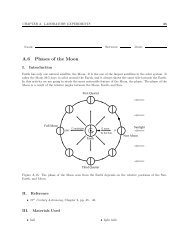
Solving Delay Differential Equations - Radford University

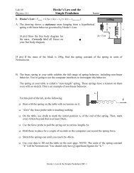
8 L.F. Shampine and S. Thompson
evaluating the DDEs (4). The lags argument is a vector of the lags τ1, . . . , τk.
There is only one lag in the example DDE, so the argument is here a scalar.
The argument tspan specifies the interval [t0, tf ] of interest. Unlike the ODE
solvers of Matlab, the DDE solvers require that t0 < tf . The third argument
is a function for evaluating the history, i.e., the solution for t ≤ t0. A
constant history function is so common that the solver allows users to supply
a constant vector instead of a function and that was done in computing the
second solution. The first two arguments of the function for evaluating the
DDEs is the same as for a system of ODEs, namely the independent variable
t and a column vector of dependent variables approximating y(t). Here the
latter is called T and is a scalar. A challenging task for the user interface is
to accomodate multiple delays. This is done with the third argument Z which
is an array of k columns. The first column approximates y(t − τ1) with τ1
defined as the first delay in lag. The second column corresponds to the second
delay, and so forth. Here there is only one delay and only one dependent
variable, so Z is a scalar. A notable difference between dde23 and ode23 is
the output, here called sol. The ODE solvers of Matlab optionally return
solutions as a complex data structure called a structure, but that is the only
form of output from the DDE solvers. The solution structure sol1 returned
by the first integration contains the mesh that was selected as the field sol1.x
and the solution at these points as the field sol1.y. With this information
the first solution can be plotted by plot(sol1.x,sol1.y). Often this is satisfactory,
but this particular problem is so easy that values of the solution
at mesh points alone does not provide a smooth graph. Approximations to
the solution can be obtained anywhere in the interval of interest by means of
the auxiliary function deval. In the example program the two solutions are
approximated at 100 equally spaced points for plotting. A marker is plotted
at (0, T (0)) to distinguish the two histories from the corresponding computed
solutions of (1). The discontinuity in the first derivative at the initial point is
clear for the history T (t) = 1, but the discontinuity in the second derivative
at t = 1 is scarcely visible.
3 Numerical Methods and Software Issues
The method of steps and modifications of methods for ODEs can be used
to solve DDEs. Because they are so popular, we study in this chapter only
explicit Runge–Kutta methods. In addition to discussing basic algorithms, we
take up important issues that arise in designing software for DDEs.
3.1 Explicit Runge–Kutta Methods
Given yn ≈ y(tn), an explicit Runge–Kutta method for a first order system
of ODEs (3) takes a step of size hn to form yn+1 ≈ y(tn+1) at tn+1 = tn + hn
as follows. It first evaluates the ODEs at the beginning of the step,