Hybrid Methods for Initial Value Problems in Ordinary Differential ...
Hybrid Methods for Initial Value Problems in Ordinary Differential ...
Hybrid Methods for Initial Value Problems in Ordinary Differential ...

Create successful ePaper yourself
Turn your PDF publications into a flip-book with our unique Google optimized e-Paper software.
HYBRID RIETHODS FOR INITIAL VALUE PROBLEMS 81<br />
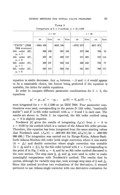
TABLE 2<br />
Comparison of k = 2 methods, x = 0(.1)200<br />
x = 100 x = 200<br />
---<br />
s<strong>in</strong> Error cos Error s<strong>in</strong> Error cos Error<br />
---<br />
"TRUE" (IBM -5063 656 8623 186 -8732 973 4871 871<br />
7094 FORTRAN)<br />
6th order (E), 506 150 051 135 575 398 795 76<br />
a1 = 1<br />
6th order (E), 557 99 059 127 671 302 757' 114<br />
a1 = 0<br />
5th order (D), 489 167 042 144 528 445 794 77<br />
a1 = 1<br />
5th order (D)! 543 113 052 134 641 332 760 111<br />
a1 = 0<br />
equation is stable decreases. Any al between -.5 and +.4 would appear<br />
to be a reasonable choice, the <strong>for</strong>mer be<strong>in</strong>g preferred if the equation is<br />
unstable, the latter <strong>for</strong> stable equations.<br />
In order to compare different parameter comb<strong>in</strong>ations <strong>for</strong> k = 2, the<br />
equations<br />
were <strong>in</strong>tegrated <strong>for</strong> x = 0(.1)200 on an IBM 7094. Four parameter com-<br />
b<strong>in</strong>ations were used, correspond<strong>in</strong>g to the po<strong>in</strong>ts D (5th order, "maximally<br />
stable") and E (a 6th order method) with a1 = 0 and 1<strong>in</strong> each case. The<br />
results are shown <strong>in</strong> Table 2. As expected, the 6th order method us<strong>in</strong>g<br />
a1 = 0 is slightly superior.<br />
Nordsieck [4] gives the results of <strong>in</strong>tegrat<strong>in</strong>g JIG(%) from x - 6 to<br />
x = 6138 by his method which is a variant of the Adams 6th order process.<br />
There<strong>for</strong>e, this equation has been <strong>in</strong>tegrated fro<strong>in</strong> the same start<strong>in</strong>g values<br />
that Nordsieck used. (Jl~(6) = .000 001 201 950; dJ1~(6)/dx = .000 002<br />
986 480.) The <strong>in</strong>tegration was carried out by Runge-Kutta, Adams-Bash-<br />
<strong>for</strong>th-Adams-Moulton 6th order [with s<strong>in</strong>gle correction where it was stable<br />
(h = &) and double correction where s<strong>in</strong>gle correction was unstable<br />
(h = & and h = Q)], by the 6th order hybrid with k = 2 correspond<strong>in</strong>g to<br />
the po<strong>in</strong>t E <strong>in</strong> Fig. 1 with al = 0, and by an 8th order method discussed <strong>in</strong><br />
the next section. The step sizes Q, & and & were used <strong>in</strong> order t)o make<br />
mean<strong>in</strong>gful comparisons with Nordsieck's method. The results that he<br />
quotes, although <strong>for</strong> variable step size, took average step sizes of Q and &.<br />
S<strong>in</strong>ce this method <strong>in</strong>volves two evaluations of the derivative, it seemed<br />
pert<strong>in</strong>ent to use Adams s<strong>in</strong>gle corrector with one derivative evaluation <strong>for</strong>