Hybrid Methods for Initial Value Problems in Ordinary Differential ...

HYBRID METHODS FOR INITIAL VALUE PROBLEMS
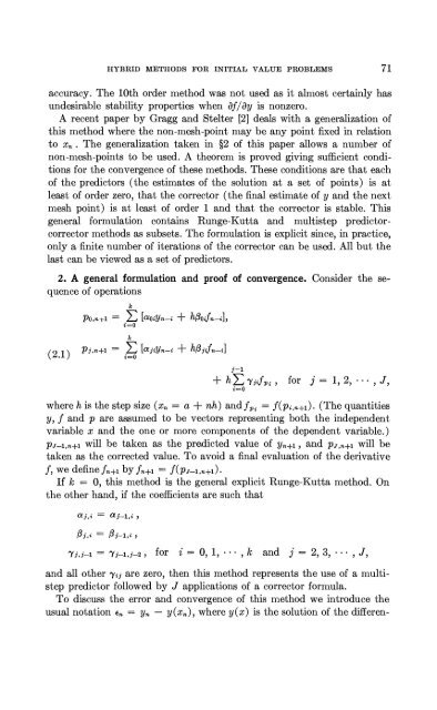
accuracy. The 10th order niethod was not used as it almost certainly has
undesirable stability properties when is nonzero.
A recent paper by Gragg and Stelter [2] deals with a generalization of
this method where the non-mesh-point niay be any point fixed in relation
to x, . The generalization taken in 82 of this paper allows a number of
non-mesh-points to be used. A theoren1 is proved giving sufficient condi-
tions for the convergence of these methods. These conditions are that each
of the predictors (the estimates of the solution at a set of points) is at
least of order zero, that the corrector (the final estimate of y and the next
mesh point) is at least of order 1 and that the corrector is stable. This
general formulation contains Runge-Kutta and nlultistep predictorcorrector
methods as subsets. The formulation is explicit since, in practice,
only a finite number of iterations of the corrector can be used. All but the
last can be viewed as a set of predictors.
2. A general formulation and proof of convergence. Consider the sequence
of operations
71
j-1
+ hCyjifpi , for j = 1, 2, -. , J,
i=O
where h is the step size (x, = a + nh) and fpi = f(pi,,+l). (The quantities
y, f and p are assumed to be vectors representing both the independent
variable x and the one or more components of the dependent variable.)
p~-~,,+~ will be taken as the predicted value of yn+l, and p,,,+, will be
taken as the corrected value. To avoid a final evaluation of the derivative
f, we define fn+lby fn+l = f(p~-l,n+l).
If k = 0, this method is the general explicit Runge-Kutta niethod. On
the other hand, if the coefficients are such that
p..- p. .
39% - ,
yj,j-1 = yj-1,j-2, for i= 0, 1, .-.,k and j = 2,3, ..., J,
and all other yii are zero, then this nlethod represents the use of a multi-
step predictor followed by J applications of a corrector formula.
To discuss the error and convergence of this method we introduce the
usual notation en = yn - y(xn), where y(x) is the solution of the differen-