Polylogarithmic identities in cubical higher Chow groups
Polylogarithmic identities in cubical higher Chow groups
Polylogarithmic identities in cubical higher Chow groups

You also want an ePaper? Increase the reach of your titles
YUMPU automatically turns print PDFs into web optimized ePapers that Google loves.
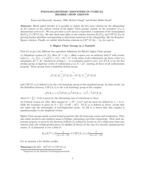
POLYLOGARITHMIC IDENTITIES IN CUBICAL<br />
HIGHER CHOW GROUPS<br />
Essen and Bayreuth, January, 1998, Herbert Gangl 1 and Stefan Müller-Stach 1<br />
Abstract: Bloch asked whether it is possible to obta<strong>in</strong> the five term relation for the dilogarithm<br />
<strong>in</strong> the context of the <strong>cubical</strong> version of his <strong>higher</strong> <strong>Chow</strong> <strong>groups</strong>, namely as the boundary of a 2dimensional<br />
cycle <strong>in</strong> A 4 . We can give such a cycle and as a byproduct a realization of the isomorphism<br />
B2(F )Q ∼ = CH 2 (F, 3)Q. We also shed some light on the relation between B3(F )Q and CH 3 (F, 5)Q by<br />
prov<strong>in</strong>g further <strong>identities</strong> correspond<strong>in</strong>g to functional equations of the trilogarithm, like the Kummer-<br />
Spence relation. F<strong>in</strong>ally, we exhibit distribution relations <strong>in</strong> CH m (F, 2m − 1)Q for each m.<br />
I. Higher <strong>Chow</strong> Groups <strong>in</strong> a Nutshell<br />
First let us give two different but equivalent def<strong>in</strong>itions for Bloch’s <strong>higher</strong> <strong>Chow</strong> <strong>groups</strong>:<br />
(1) Simplicial version (cf. [1]): Here ∆n = An F = aff<strong>in</strong>e n-space over an arbitrary field F with coord<strong>in</strong>ates<br />
t0, ..., tn, ti = 1 and Σ = ∪{ti = 0} ⊂ An is the union of all codimension one faces; a face is a<br />
subsimplex ∆m ⊂ ∆n obta<strong>in</strong>ed by sett<strong>in</strong>g n − m coord<strong>in</strong>ates equal to zero. Let Z p (X, n) be the free<br />
abelian group of algebraic cycles of codimension p on X × ∆n , meet<strong>in</strong>g all faces of all codimensions<br />
properly. These <strong>groups</strong> form a simplicial abelian group:<br />
...Z r →<br />
→<br />
(X, 3) Z<br />
→<br />
→<br />
r →<br />
(X, 2) → Z<br />
→<br />
r (X, 1) →<br />
→ Zr (X, 0)<br />
and CH p (X, n) is def<strong>in</strong>ed to be the n-th homotopy group of this simplicial group. In other words, via<br />
the Dold-Kan theorem, CH p (X, n) is the n-th homology group of the complex<br />
...Z p (X, n + 1) ∂ →Z p (X, n) ∂ →Z p (X, n − 1) ∂ →... ∂ →Z p (X, 0)<br />
where ∂ = (−1) i ∂i is given by the alternat<strong>in</strong>g sum of restrictions to faces.<br />
(2) Cubical version (cf. [10]): Here <strong>in</strong>stead A n = (P 1 \ {1}) n and the faces are def<strong>in</strong>ed by xi = 0, ∞,<br />
while the boundary is given by ∂ = (−1) i (∂ 0 i − ∂∞ i ). Zp (X, n) is def<strong>in</strong>ed as above, except that<br />
one takes only the subcomplex of non-degenerate cycles. In [10] it is shown that this complex is<br />
quasiisomorphic to the simplicial version.<br />
Higher <strong>Chow</strong> <strong>groups</strong> satisfy several formal properties like the homotopy axiom and localization. They<br />
also admit products and regulator maps to Deligne cohomology and étale cohomology. Their most important<br />
property is given by the theorem of Bloch [1] (ref<strong>in</strong>ed by Lev<strong>in</strong>e <strong>in</strong> [11]) which puts them <strong>in</strong>to<br />
relation with (the weight-graded pieces of) Quillen K-theory <strong>in</strong> the case of a smooth, quasiprojective<br />
variety X of dimension d over a field F :<br />
Let us mention a few further results:<br />
Kn(X) (p) 1<br />
⊗ Z[<br />
(n + d − 1)! ] ∼ = CH p 1<br />
(X, n) ⊗ Z[<br />
(n + d − 1)! ]<br />
Theorem([13],[16]). K M n (F ) ∼ = CH n (F, n).<br />
1 Supported by the Deutsche Forschungsgeme<strong>in</strong>schaft<br />
1
Theorem([14]). CH 2 (F, 3) = K <strong>in</strong>d<br />
3 (F ) = K3(F )/K M 3 (F ).<br />
Modulo torsion both sides are isomorphic to the Bloch group B2(F ) .<br />
II. Computations <strong>in</strong> CH m (F, 2m − 1).<br />
We work <strong>in</strong> <strong>cubical</strong> coord<strong>in</strong>ates. Let G = Gn be the wreath product of the symmetric group<br />
Sn and (Z/2Z) n . It acts on Z p (F, n) ⊗ Q via permutation and <strong>in</strong>version of coord<strong>in</strong>ates. Def<strong>in</strong>e<br />
sgn : Sn → Z/2Z and sgn j : Z/2Z → Z/2Z to be the non-trivial 1-dimensional characters and<br />
χ = sgn ·<br />
then there is a natural choice of an idempotent<br />
n<br />
sgnj ,<br />
j=1<br />
Altn : Z p (F, n) ⊗ Q → Z p (F, n) ⊗ Q , Z ↦→ 1<br />
|G|<br />
<br />
χ(g) g(Z) ,<br />
Note that we abbreviate Altn and sometimes Alt (when the context is clear) for the alternation over<br />
the full group G. Def<strong>in</strong>e C p (F, n) ⊂ Z p (F, n) ⊗ Q to be the image of Alt together with the differential<br />
<strong>in</strong>duced by ∂. The result<strong>in</strong>g homological complex<br />
C m (F, ·) : . . . → C m (F, 2m) → C m (F, 2m − 1) → . . . → C m (F, m) → 0<br />
still computes CH m (F, n)Q by [10].<br />
I. First let m = 2: the complex C 2 (F, ·) has the acyclic subcomplex<br />
. . . → C 1 (F, 1) ∧ C 1 (F, 3) → C 1 (F, 1) ∧ C 1 (F, 2) → C 1 (F, 1) ∧ ∂C 1 (F, 2) → 0 ,<br />
i.e. the truncation of the subcomplex consist<strong>in</strong>g of subvarieties where one coord<strong>in</strong>ate entry is constant.<br />
The proof of acyclicity is the same as <strong>in</strong> [12]. The quotient complex will be denoted by A 2 (F, ·). It<br />
is quasiisomorphic to C 2 (F, ·) and has certa<strong>in</strong> advantages; for example cycles <strong>in</strong> C 2 (F, 3) with one<br />
coord<strong>in</strong>ate entry be<strong>in</strong>g constant have zero image <strong>in</strong> A 2 (F, 3). We call such cycles negligible. Another<br />
advantage is—due to the fact that we mod out C 2 (F, 2) by C 1 (F, 1) ∧ ∂C 1 (F, 2)—that the follow<strong>in</strong>g<br />
diagram is well-def<strong>in</strong>ed and commutative:<br />
Z[F − {0, 1}]<br />
ρ2<br />
<br />
A2 (F, 3)<br />
∂A2 (F, 4)<br />
β2 <br />
∂ <br />
2 F ∗<br />
g∈G<br />
id⊗id<br />
<br />
2 A (F, 2)<br />
where for a group G we denote by 2 G the subgroup of G ⊗ G generated by {a ⊗ b − b ⊗ a | a, b ∈ G}.<br />
The map β2 is given on generators as [a] ↦→ a ⊗ (1 − a) − (1 − a) ⊗ a.<br />
The map ρ2 is def<strong>in</strong>ed as ρ2(a) = Ca mod ∂A 2 (F, 4) for a ∈ F ∗ , where Ca is def<strong>in</strong>ed <strong>in</strong> (2) below.<br />
Notation: Given a rational map ϕ : (P 1 ) d → (P 1 ) n , we let Nϕ be the cycle associated to ϕ,<br />
Nϕ := ϕ∗<br />
<br />
(P 1 ) d<br />
∩ n ,<br />
2<br />
(1)
i.e. the direct image <strong>in</strong> the sense of Fulton (1.4) [6].<br />
For mnemonic reasons (cube=[ ]) we propose a “<strong>cubical</strong>” notation<br />
[ϕ1(x), . . . , ϕn(x)] , x = (x1, . . . , xn),<br />
for Altn(N (ϕ1(x),...,ϕn(x))).<br />
By abuse of notation, we will often identify ϕ with Nϕ , and we <strong>in</strong>troduce the further abbreviation for<br />
parametrized cycles of the special form associated to a rational function f<br />
<br />
Zf = Alt3 N(x,1−x,f(x)) .<br />
F<strong>in</strong>ally, we return to the def<strong>in</strong>ition of Ca (cf. [16]) as<br />
Ca = Z x−a<br />
x<br />
= [x, 1 − x,<br />
x − a<br />
] . (2)<br />
x<br />
Note: In the follow<strong>in</strong>g, equality signs between cycles are understood modulo negligible terms.<br />
Lemma 1: Let f, g, r and s be rational functions <strong>in</strong> one variable. Then there exists an element<br />
W ∈ A2 (F, 4) with<br />
<br />
<br />
∂W = f(x), g(x), r(x)s(x) − [f(x), g(x), r(x)] − [f(x), g(x), s(x)] .<br />
if all three cycles on the right hand side are admissible, i.e. <strong>in</strong>tersect all faces <strong>in</strong> the correct dimension.<br />
Proof. Let W be the parametrized cycle W := [f(x), g(x), y−r(x)s(x)<br />
y−r(x) , y]. Then we compute (denot<strong>in</strong>g<br />
the coord<strong>in</strong>ates by x1, . . . , x4) that W ∩ {x1 = 0}, W ∩ {x1 = ∞}, W ∩ {x2 = 0} and W ∩ {x2 = ∞}<br />
are negligible, s<strong>in</strong>ce one coord<strong>in</strong>ate entry becomes constant. Next, W ∩ {x4 = ∞} = ∅, s<strong>in</strong>ce the third<br />
coord<strong>in</strong>ate becomes 1. The rema<strong>in</strong><strong>in</strong>g three boundaries give the three terms <strong>in</strong> the assertion. <br />
Corollary 1. (a) Ca + C1−a = C1 <strong>in</strong> A 2 (F, 3)/∂A 2 (F, 4).<br />
(b) Consider, for arbitrary e, f ∈ F × , the cycle W (a, b, c, d) : x ↦→ [ x−a x−b x−c<br />
e , f , x−d ] for pairwise<br />
dist<strong>in</strong>ct elements a, b, c, d ∈ F . Then<br />
W (a, b, c, d) = C c−a<br />
b−a<br />
− C d−a ∈ A<br />
b−a<br />
2 (F, 3)/∂A 2 (F, 4)<br />
Furthermore,<br />
[x, 1 − x a<br />
, 1 −<br />
b x ] = C a<br />
b ∈ A2 (F, 3)/∂A 2 (F, 4) .<br />
Proof: (a) We apply Lemma 1 with f(x) = x, g(x) = 1 − x, r(x) = x−a<br />
x−1<br />
x−1 and s(x) = x to obta<strong>in</strong><br />
Ca = Z x−a<br />
x<br />
yields<br />
= Z x−a<br />
x−1<br />
+ C1. Substitut<strong>in</strong>g x ↦→ (1 − x) and permut<strong>in</strong>g the first two components <strong>in</strong> Z x−a<br />
x−1<br />
<br />
x − a<br />
<br />
1 − x − a<br />
<br />
x − (1 − a)<br />
<br />
x, 1 − x, = 1 − x, x, = − x, 1 − x, = −C1−a .<br />
x − 1<br />
−x<br />
x<br />
(b) We only prove the first assertion (the second can be shown <strong>in</strong> a similar way), and we restrict to<br />
the case e = f = 1. The general case can be easily deduced by repeat<strong>in</strong>g some of the arguments used.<br />
W (a, b, c, d) = W (0, b − a, c − a, d − a) by the transformation x ↦→ x + a. However<br />
W (0, b − a, c − a, d − a) = [x, 1 − x x + a − c<br />
,<br />
b − a x + a − d ]<br />
1 x+a−c<br />
(here we multiplied with the admissible cycle [x, a−b , x+a−d ] ∈ C1 (F, 1) ∧ C1 (F, 2), which is allowed<br />
by lemma 1 <strong>in</strong> view of the def<strong>in</strong>ition of A 2 (F, ·)) and therefore, us<strong>in</strong>g the transformation x ↦→ (b − a)x,<br />
W (0, b − a, c − a, d − a) = [(b − a)x, 1 − x,<br />
3<br />
c−a x − b−a<br />
x − d−a<br />
b−a<br />
] ,
whence it ensues that it is equal (up to an admissible cycle <strong>in</strong> C 1 (F, 1) ∧ C1 (F, 2)) to<br />
c−a<br />
c−a<br />
x − b−a<br />
x − b−a<br />
[x, 1 − x, ] = [x, 1 − x, ] − [x, 1 − x,<br />
x<br />
x − d−a<br />
b−a<br />
d−a x − b−a<br />
] = C c−a − C d−a . <br />
x<br />
b−a b−a<br />
We proceed to describe the geometric nature of certa<strong>in</strong> functional equations for the dilogarithm <strong>in</strong> the<br />
realm of <strong>higher</strong> <strong>Chow</strong> <strong>groups</strong>.<br />
Theorem 1: (a) If F conta<strong>in</strong>s a primitive n-th root of unity, then every a ∈ F ∗ gives rise to a<br />
distribution relation:<br />
<br />
nCan = n2<br />
ζn Cζa <strong>in</strong> A<br />
=1<br />
2 (F, 3)/∂A 2 (F, 4)<br />
(b) For a = b, 1 − b, and a, b = 0, 1, one obta<strong>in</strong>s the five term relation<br />
Va,b := C a(1−b) − C 1−b + C1−b − C a<br />
b(1−a) 1−a<br />
b + Ca = 0 ∈ A 2 (F, 3)/∂A 2 (F, 4) .<br />
(c) The <strong>in</strong>version relation holds:<br />
2(Ca + C 1<br />
a − 2C1) = 0 ∈ A 2 (F, 3)/∂A 2 (F, 4) .<br />
(d) Let f : P1 → P1 be any rational function of degree n. Then the follow<strong>in</strong>g relation holds:<br />
2n 2 Ccr(f(x),a,b,c) = 2n <br />
Ccr(x,α,β,γ) γ∈f −1 (c) β∈f −1 (b) α∈f −1 (a)<br />
assum<strong>in</strong>g that x, a, b, c ∈ F and all α, β, γ are mutually dist<strong>in</strong>ct and lie <strong>in</strong> F .<br />
Here cr(a, b, c, d) denotes the cross ratio (a−c)(b−d)<br />
(a−d)(b−c) .<br />
Proof: (a) We give the proof for n = 2: note that 2C a 2 = [t 2 , 1 − t 2 , t2 −a 2<br />
t2 ] (cf. [6], 1.4). Therefore<br />
by repeated application of Lemma 1 (check that <strong>in</strong> each step all cycles are def<strong>in</strong>ed, i.e. admissible):<br />
2Ca2 = [t2 , 1 − t2 , t2−a 2<br />
t2 ] = [t2 , 1 − t2 , t−a<br />
t ] + [t2 , 1 − t2 , t+a<br />
t ]<br />
= [t2 , 1 − t, t−a<br />
t ] + [t2 , 1 + t, t−a<br />
t ] + [t2 , 1 − t, t+a<br />
t ] + [t2 , 1 + t, t+a<br />
= [t2 , 1 − t, t−a<br />
t ] + [t2 , 1 − t, t+a<br />
t ] + [t2 , 1 − t, t+a<br />
t ] + [t2 , 1 − t, t−a<br />
= 4[t, 1 − t, t−a<br />
t ] + 4[t, 1 − t, t+a<br />
t ]<br />
= 4Ca + 4C−a .<br />
For n ≥ 3, the proof is similar, not<strong>in</strong>g that nCan = [tn , 1 − tn , tn−a n<br />
tn t n − a n = (t − ζa).<br />
t ]<br />
t ]<br />
] and 1 − t n = (1 − ζt) and<br />
(b) In table 1 a proof of the five term relation is given both <strong>in</strong> terms of cycles and (parallel to it)<br />
<strong>in</strong> terms of graphs; the latter visualize (and guide) the decomposition of cycles. One can play the<br />
follow<strong>in</strong>g game: start<strong>in</strong>g from a “dist<strong>in</strong>guished position” (this corresponds to a sum of cycles Cai),<br />
one is allowed to perform a number of “moves” (this corresponds to decompos<strong>in</strong>g the cycles) of a<br />
certa<strong>in</strong> k<strong>in</strong>d which should eventually lead to another “dist<strong>in</strong>guished position” (aga<strong>in</strong>, a sum Cbj ).<br />
If the latter is different from the start<strong>in</strong>g position, the difference [ai] − [bj] gives a functional<br />
equation for the dilogarithm. The (undirected) graph encodes certa<strong>in</strong> data of cycles whose coord<strong>in</strong>ates<br />
are products of fractional l<strong>in</strong>ear transformations: we fix an order<strong>in</strong>g of the coord<strong>in</strong>ates; the zeros of a<br />
coord<strong>in</strong>ate are marked po<strong>in</strong>ts which are connected via marked edges to its poles—also given as marked<br />
po<strong>in</strong>ts. The mark underneath a po<strong>in</strong>t denotes the po<strong>in</strong>t viewed as ly<strong>in</strong>g <strong>in</strong> P 1 , the encircled number<br />
above an edge gives the number of the coord<strong>in</strong>ate <strong>in</strong> the chosen order<strong>in</strong>g of the cycle coord<strong>in</strong>ates.<br />
E.g. if the second coord<strong>in</strong>ate is given by 1 − x, it is encoded as<br />
4
2<br />
• • .<br />
1 ∞<br />
The other <strong>in</strong>formation which is captured <strong>in</strong> the graph are the preimages of 1, these are pictured by<br />
a full-square with both the mark<strong>in</strong>g of the po<strong>in</strong>t (below) and the <strong>in</strong>formation about the coord<strong>in</strong>ate<br />
number <strong>in</strong>side the square. In the above example we get 0 for the second coord<strong>in</strong>ate, and this results<br />
<strong>in</strong> the picture 2 .<br />
0<br />
A dotted square <strong>in</strong> the example above means that none of the coord<strong>in</strong>ates <strong>in</strong>volved has image 1<br />
at this po<strong>in</strong>t.<br />
Fractional l<strong>in</strong>ear cycles are admissible if and only if <strong>in</strong> their correspond<strong>in</strong>g graph any two adjacent<br />
edges are “glued” along a full-squared vertex (as opposed to a dotted-squared one). The latter condition<br />
corresponds <strong>in</strong> the language of cycles to boundary terms which have one coord<strong>in</strong>ate be<strong>in</strong>g 0 or<br />
∞ (and are a priori not admissible) but which are annihilated s<strong>in</strong>ce another coord<strong>in</strong>ate is equal to 1<br />
and therefore vanishes.<br />
A dist<strong>in</strong>guished position is of the type • , the <strong>in</strong>formation about coord<strong>in</strong>ates<br />
is essentially redundant (but convenient for purposes of comparison as <strong>in</strong> the table).<br />
A move is one of the follow<strong>in</strong>g: (1) split up an edge <strong>in</strong>to two, (2) move a full square from one vertex<br />
to another, and (3) the reverse operations to (1) and (2).<br />
A move is admissible if both graphs before and after the move are admissible.<br />
We could also <strong>in</strong>troduce a direction of the graph, say, by substitut<strong>in</strong>g edges by arrows go<strong>in</strong>g from<br />
a zero to a pole and then we can give it a sign, depend<strong>in</strong>g on the permutation of the encircled marks<br />
and the direction of the arrows. This will determ<strong>in</strong>e a cycle unambiguously from its graph. S<strong>in</strong>ce we<br />
can get by without and we don’t want to overload the picture, we omit it.<br />
(c) follows from (b) and of corollary 1, (a):<br />
Va,b + V 1 1<br />
a , b − (Cb + C1−b − C1) − (C 1<br />
b + C1− 1<br />
b − C1) = Ca + C 1<br />
a − Cb − C 1<br />
b − (C a + C b − 2C1) .<br />
b a<br />
Now add the correspond<strong>in</strong>g expression where the roles of a and b are <strong>in</strong>terchanged.<br />
(d) For simplicity we restrict to the case of f(x) be<strong>in</strong>g a polynomial of degree n and tak<strong>in</strong>g a, b, c ∈ F<br />
such that all their preimages are dist<strong>in</strong>ct (i.e. they are non-critical po<strong>in</strong>ts of the map f). Then for<br />
any α and β such that f(α) = a, f(β) = b, the follow<strong>in</strong>g decompositions hold:<br />
f(x) − a<br />
b − a =<br />
<br />
i (x − αi)<br />
,<br />
(β − αi)<br />
i<br />
f(x) − b<br />
a − b =<br />
<br />
(x − βj)<br />
j<br />
<br />
j<br />
(α − βj)<br />
Therefore reparametriz<strong>in</strong>g nCc, us<strong>in</strong>g x ↦→ f(x)−a<br />
b−a , gives<br />
i<br />
and<br />
(x − αi) f(x) − b<br />
nCc =<br />
,<br />
(β − αi) a − b ,<br />
<br />
k (x − γk)<br />
<br />
<br />
(x − αl)<br />
and we can decompose <strong>in</strong> the first coord<strong>in</strong>ate <strong>in</strong> the follow<strong>in</strong>g way<br />
= <br />
x − αi<br />
,<br />
β − αi<br />
f(x) − b<br />
a − b ,<br />
<br />
k (x − γk)<br />
<br />
<br />
(x − αl)<br />
i<br />
l<br />
l<br />
f(x) − c<br />
f(x) − a =<br />
<br />
k (x − γk)<br />
.<br />
(x − αl)<br />
s<strong>in</strong>ce all the result<strong>in</strong>g cycles are admissible, and furthermore, we can decompose <strong>in</strong> the last coord<strong>in</strong>ate<br />
which for convenience we write as a double product (which is matched up by a factor n on the left)<br />
n 2 Cc = <br />
x − αi<br />
,<br />
β − αi<br />
f(x) − b x −<br />
<br />
γk<br />
, .<br />
a − b x − αl<br />
i,k,l<br />
6<br />
l
Now we need to dist<strong>in</strong>guish two cases i = l and i = l. The latter one poses no problem, we can<br />
, and a typical cycle<br />
decompose <strong>in</strong> the second coord<strong>in</strong>ate <strong>in</strong>to terms x−βj<br />
α−βj<br />
<br />
x − αi<br />
,<br />
β − αi<br />
x − βj<br />
,<br />
α − βj<br />
x − γk<br />
<br />
x − αl<br />
is admissible and—via corollary 1(b)—equivalent to C γ k −α i<br />
β j −α i<br />
− C αl−αi .<br />
βj −αi For the terms with i = l we only need to decompose the second coord<strong>in</strong>ate <strong>in</strong>to factors x−βj<br />
αi−βj with<br />
<br />
−1 the same αi above we could have chosen any α ∈ f (a) to make sure of the admissibility of the<br />
. This gives us the<br />
result<strong>in</strong>g cycles, and then we can aga<strong>in</strong> <strong>in</strong>voke corollary 1(b) to obta<strong>in</strong> C γ k −α i<br />
β j −α i<br />
claim with a polynomial f, s<strong>in</strong>ce two terms t(i, l) = C α l −α i<br />
β j −α i<br />
that 2(Cx + C x<br />
x−1<br />
and t(l, i) are equal up to 2-torsion (note<br />
) = 0, which follows from (c) and corollary 1(a)). <br />
Corollary 2. C1 = C−1 = 0 ∈ CH 2 (F, 3)Q.<br />
Proof: Use (a) with n = 2 and (c) with a = −1, respectively. The outcome is 4C−1 = 4C1 and<br />
4C−1 = −2C1, yield<strong>in</strong>g 6C1 = 12C−1 = 0. <br />
Return<strong>in</strong>g to diagram (1), we see that the map <strong>in</strong>duced by ρ2 on the kernels factors (up to tensor<strong>in</strong>g<br />
with Q) through the Bloch group B2(F ) (which is def<strong>in</strong>ed [14] as the quotient of ker β2 by<br />
the subgroup generated by the five term relation), thereby realis<strong>in</strong>g the well-known isomorphism<br />
B2(F )Q ∼ = CH 2 (F, 3)Q.<br />
II. Now let m ≥ 3. Consider the cycles of Bloch-Kriz ([2])<br />
Ca = C (m)<br />
<br />
a : (x1, ..., xm−1) ↦→ x1, ..., xm−1, 1 − x1, 1 − x2<br />
, ..., 1 −<br />
x1<br />
xm−1<br />
, 1 −<br />
xm−2<br />
a<br />
<br />
xm−1<br />
<strong>in</strong> C m (F, 2m − 1) (m will be clear from the context so we suppress the superscript).<br />
As <strong>in</strong> the case m = 2 we modify the complex C m (F, ·) <strong>in</strong> such a way that we can manipulate<br />
parametrized cycles modulo negligible ones. To simplify our computations a little bit, we mod out by<br />
a subcomplex J m (F, ·) which was already considered by Bloch and Kriz <strong>in</strong> [2]. It can be constructed<br />
as follows: look first at the graded algebra<br />
<br />
C p (F, n)<br />
p,n<br />
with multiplication given by the product <strong>in</strong> <strong>cubical</strong> coord<strong>in</strong>ates (see [11]). The differential graded<br />
ideal generated by all C p (F, n) with n ≥ 2p + 1 and all C p (F, 2p) for p ≥ 1 is denoted by J · (F, ·). It<br />
conta<strong>in</strong>s for example all <strong>groups</strong> ∂C p (F, 2p) for p ≥ 1.<br />
For m = 3, the group J 3 (F, 5) conta<strong>in</strong>s the sub<strong>groups</strong><br />
J 3 (F, 4) conta<strong>in</strong>s the sub<strong>groups</strong><br />
C 1 (F, 1) ∧ C 2 (F, 4), C 1 (F, 2) ∧ C 2 (F, 3) and ∂C 3 (F, 6).<br />
∂C 1 (F, 2) ∧ C 2 (F, 3), C 1 (F, 1) ∧ ∂C 2 (F, 4) and C 1 (F, 2) ∧ C 2 (F, 2).<br />
7
The quotient complex C 3 (F, ·)/J 3 (F, ·) will be denoted by A 3 (F, ·). For number fields F , the complex<br />
J 3 (F, ·) is known to be acyclic, so A 3 (F, ·) is quasiisomorphic to C 3 (F, ·) <strong>in</strong> this case. This is a<br />
consequence of Borel’s theorem [4] by us<strong>in</strong>g the formulas for the regulator <strong>in</strong> [8].<br />
In general, the acyclicity of J 3 (F, ·) is not known and is related to the Beil<strong>in</strong>son-Soulé conjecture for<br />
m = 2 (cf. [2] and [15]).<br />
In the follow<strong>in</strong>g we will frequently omit terms which are conta<strong>in</strong>ed <strong>in</strong> J 3 (F, ·) and call them—as<br />
the correspond<strong>in</strong>g ones <strong>in</strong> the case m = 2—negligible. As before, equality signs between cycles are<br />
understood modulo negligible terms.<br />
We have aga<strong>in</strong> a commutative diagram<br />
Z[F − {0, 1}]<br />
ρ3<br />
<br />
A3 (F, 5)<br />
∂A3 (F, 6)<br />
β3 <br />
∂ <br />
Z[F − {0, 1}]<br />
R2(F )<br />
ρ2∧id<br />
<br />
3<br />
A (F, 4)<br />
Here R2(F ) is def<strong>in</strong>ed as the subgroup generated by five term relations.<br />
The map β3 is def<strong>in</strong>ed on generators as [a] ↦→ [a] mod R2(F ) ∧ a.<br />
The map ρ3 is def<strong>in</strong>ed as [a] ↦→ Ca = C (3)<br />
a .<br />
The next lemma tells us how far the decomposition of certa<strong>in</strong> cycles is from be<strong>in</strong>g bounded by some<br />
admissible cycle.<br />
Lemma 4: Consider a parametrized cycle of the form<br />
[f1(x), f2(y), f3(x), f4(x, y), f5(y)]<br />
where all fi are rational functions and f4 is a product of fractional l<strong>in</strong>ear transformations when<br />
considered as a function <strong>in</strong> the variable y.<br />
(a) Assume that we can write f1(x) = g(x)h(x) for some rational functions g and h. Then the<br />
admissible cycle<br />
W := [<br />
∧ F ∗<br />
z − g(x)h(x)<br />
, z, f2(y), f3(x), f4(x, y), f5(y)] ∈ A<br />
z − g(x)<br />
3 (F, 6)<br />
gives the follow<strong>in</strong>g relation (provided all terms are admissible):<br />
∂(W ) = [f1(x), f2, f3, f4, f5] − [g(x), f2, f3, f4, f5] − [h(x), f2, f3, f4, f5]<br />
+ <br />
div(f4)<br />
±[<br />
z − g(x)h(x)<br />
, z, f2(y(x)), f3(x), f5(y(x))],<br />
z − g(x)<br />
where we solve the equations f4(x, y) = 0 (coefficient is +1) and 1/f4(x, y) = 0 (coefficient is −1) by<br />
the implicit function y(x) <strong>in</strong> terms of x. Specifically, if e.g. f2(y(x)) = f3(x), the correspond<strong>in</strong>g term<br />
<strong>in</strong> the latter sum vanishes under the alternation.<br />
A similar relation holds if we decompose fi for i = 4 <strong>in</strong>to two factors.<br />
(b) In the case i = 4, assume that we can write f4(x, y) = g(x, y)h(x, y) for some rational functions g<br />
and h. Then there is an admissible cycle W ∈ A 3 (F, 6) such that<br />
∂(W ) = [f1, f2, f3, f4(x, y), f5] − [f1, f2, f3, g(x, y), f5] − [f1, f2, f3, h(x, y), f5] ,<br />
8<br />
(3)
provided that all occurr<strong>in</strong>g terms are admissible.<br />
(c) Assume for each solution y = r(x) of f4(x, y) = 0 that f1(x) = f2(r(x)) = g(x)h(x) and that<br />
either g(r(x)) = g(x) or g(r(x)) = h(x).<br />
Introduce a shorthand Z(e1, e2) = [e1(x), e2(y), f3(x), f4(x, y), f5(y)] for any two functions e1, e2 <strong>in</strong><br />
one variable. Then<br />
2Z(f1, f2) = Z <br />
g, f2 + Z h, f2 + Z f1, g + Z f1, h <br />
and<br />
2Z(f1, f2) = 2 Z(g, g) + Z(g, h) + Z(h, g) + Z(h, h) .<br />
Proof. (a) The first three boundaries W ∩ {x1 = 0} , W ∩ {x1 = ∞} and W ∩ {x2 = 0} produce<br />
the terms [f1(x), f2, f3, f4, f5] − [g(x), f2, f3, f4, f5] − [h(x), f2, f3, f4, f5]. Then W ∩ {x2 = ∞} = ∅,<br />
s<strong>in</strong>ce the first coord<strong>in</strong>ate becomes 1. The next four boundaries W ∩ {x3 = 0} , W ∩ {x3 = ∞},<br />
W ∩{x4 = 0} and W ∩{x4 = ∞} are <strong>in</strong> J 3 (F, 5) and therefore negligible. The boundaries W ∩{x5 = 0}<br />
and W ∩ {x5 = ∞} create the sum <br />
div(f4)<br />
boundaries W ∩ {x6 = 0} and W ∩ {x6 = ∞} are aga<strong>in</strong> negligible.<br />
(b) is easier to prove than (a) and therefore left to the reader.<br />
(c) The first equation follows by us<strong>in</strong>g the boundaries of the cycle<br />
±[ z−g(x)h(x)<br />
z−g(x) , z, f2(y(x)), f3(x), f5(y(x))]. The last two<br />
[ z − f1(x)<br />
z − g(x) , z, f2(y),<br />
z − f2(y)<br />
f3(x), f4(x, y), f5(y)] − [f1(x),<br />
z − g(y) , z, f3(x), f4(x, y), f5(y)] ,<br />
and not<strong>in</strong>g that the “deviation terms” (as given <strong>in</strong> (a)) from the decomposition are the same for both<br />
summands up to alternation. So they cancel <strong>in</strong> the difference and we are left with<br />
Z <br />
g, f2 + Z h, f2 + Z f1, g + Z f1, h − 2Z(f1, f2) = 0 .<br />
For the second equation, one uses the first one and the boundaries of the cycles<br />
[ z − f1(x)<br />
z − g(x) , z, g(y), f3(x),<br />
z − f1(x)<br />
f4(x, y), f5(y)] + [<br />
z − g(x) , z, h(y), f3(x), f4(x, y), f5(y)] and<br />
[g(x),<br />
z − f2(y)<br />
z − g(y) , z, f3(x),<br />
z − f2(y)<br />
f4(x, y), f5(y)] + [h(x),<br />
z − g(y) , z, f3(x), f4(x, y), f5(y)] .<br />
where aga<strong>in</strong> all the “deviation terms” cancel under the alternation. <br />
Theorem 2: (a) The Kummer-Spence relation for the trilogarithm<br />
S(a, b) := C b(1−b) + C a(1−b) + C (1−a)(1−b) − 2C b − 2C 1−b − 2C b − 2C 1−b + 2C 1 + 2C 1<br />
a(1−a) b(1−a)<br />
ab<br />
a<br />
a<br />
1−a<br />
1−a<br />
1−a a − 2C1− 1<br />
b<br />
holds <strong>in</strong> the form 4 S(a, b) = 0 <strong>in</strong> A 3 (F, 5)/∂A 3 (F, 6) whenever a = b, 1 − b, and a, b = 0, 1.<br />
(b) The <strong>in</strong>version relation and the “3-term relation” hold<br />
4(Ca − C 1<br />
a ) = 0 4(Ta − Tb) = 0 , for Ta = Ca + C 1<br />
1−a + C 1− 1<br />
a .<br />
Proof: (a) All cycles <strong>in</strong>volved will be admissible.<br />
If we use a phrase like “decompose the ith coord<strong>in</strong>ate uv of a cycle <strong>in</strong>to u and v”, it is understood<br />
that there is an admissible cycle whose boundary is just the difference of the given cycle and the (sum<br />
of the) result<strong>in</strong>g ones after formally replac<strong>in</strong>g the ith coord<strong>in</strong>ate by u and v.<br />
9
Let ϕ1(x) = x(1−x)<br />
a(1−a) , ϕ2(x) = a(1−x)<br />
x(1−a) and ϕ3(x) = (1−a)(1−x)<br />
ax . Reparametriz<strong>in</strong>g Cϕ1(b) via x ↦→ ϕ1(x),<br />
y ↦→ ϕ1(y) produces the factor (deg ϕ1) 2 = 4 <strong>in</strong> the follow<strong>in</strong>g equality<br />
4Cϕ1(b) = [ϕ1(x), ϕ1(y), 1 − ϕ1(x), 1 − ϕ1(y) ϕ1(b)<br />
, 1 − ] .<br />
ϕ1(x) ϕ1(y)<br />
We apply lemma 4(c) twice to this cycle, first with u(x) = x(1−x), thereby gett<strong>in</strong>g rid of the constants<br />
a(1 − a) <strong>in</strong> the first two coord<strong>in</strong>ates, and then with u(x) = x, yield<strong>in</strong>g four cycles all of which are the<br />
same after reparametrization, namely<br />
[x, y, (1 − x x<br />
)(1 −<br />
a 1 − a<br />
y y<br />
), (1 − )(1 −<br />
x 1 − x<br />
b b<br />
), (1 − )(1 − )] .<br />
y 1 − y<br />
Us<strong>in</strong>g lemma 4(b), we decompose the fourth coord<strong>in</strong>ate <strong>in</strong>to 1− y<br />
y<br />
x and 1− 1−x , leav<strong>in</strong>g us with Z1+Z2,<br />
where<br />
Z1 = [x, y, (1 − x x y b b<br />
a )(1 − 1−a ), 1 − x , (1 − y )(1 − 1−y )] and<br />
Z2 = [x, y, (1 − x x<br />
y b b<br />
a )(1 − 1−a ), 1 − 1−x , (1 − y )(1 − 1−y )] .<br />
S<strong>in</strong>ce we had four such cycles, we obta<strong>in</strong> 4C ϕ1(b) = 4(Z1 + Z2).<br />
We will now construct Z2 <strong>in</strong> a different way, us<strong>in</strong>g ϕ2(b) and ϕ3(b), and then subtract the outcome<br />
from the one above. Consider<br />
C ϕ2(b) = a(1 − x)<br />
x(1 − a)<br />
a(1 − y) x − a y − x<br />
, , ,<br />
y(1 − a) x(1 − a) y(1 − x) ,<br />
b − y <br />
b(1 − y)<br />
and use, like above, lemma 4(c) with u = a/(1 − a) to get rid of the constants <strong>in</strong> the first two<br />
coord<strong>in</strong>ates. Then we apply lemma 4(a) to decompose the third coord<strong>in</strong>ate <strong>in</strong>to x−a 1<br />
1−a and x . Note<br />
that the cycle with 1<br />
x is just C1−b−1 (to be precise, we need lemma 4(c) aga<strong>in</strong> with u = −1).<br />
The same procedure applies to Cϕ3(b), the only difference is that the role of a and 1 − a <strong>in</strong> the third<br />
coord<strong>in</strong>ate are <strong>in</strong>terchanged.<br />
We aga<strong>in</strong> <strong>in</strong>voke lemma 4(a), not<strong>in</strong>g that f1(x) = f2(y(x)) for y(x) = x, and we can “merge” the two<br />
rema<strong>in</strong><strong>in</strong>g cycles <strong>in</strong> the third coord<strong>in</strong>ate to<br />
1 − x<br />
x<br />
1 − y<br />
, ,<br />
y<br />
x − a<br />
1 − a<br />
x − 1 + a<br />
· ,<br />
a<br />
y − x<br />
Successive decomposition of the fourth coord<strong>in</strong>ate <strong>in</strong>to y−x<br />
1−x<br />
then of the fifth coord<strong>in</strong>ate <strong>in</strong>to b−y 1<br />
1−y and b<br />
one non-negligible cycle<br />
1 − x<br />
x<br />
1 − y<br />
, ,<br />
y<br />
x − a<br />
1 − a<br />
y(1 − x) ,<br />
and 1<br />
y<br />
b − y <br />
.<br />
b(1 − y)<br />
(the second one is negligible), and<br />
(aga<strong>in</strong>, the second one is negligible) leaves us with only<br />
x − 1 + a<br />
· ,<br />
a<br />
y − x<br />
1 − x<br />
b − y <br />
, ,<br />
1 − y<br />
which now f<strong>in</strong>ally can be decomposed <strong>in</strong> the first two coord<strong>in</strong>ates via lemma 4(c) with u(x) = 1 − x<br />
<strong>in</strong>to four terms Ti given (after an obvious reparametrization) by<br />
= x, y, (1 − x<br />
1 − a<br />
− x, y, (1 − x<br />
1 − a<br />
)(1 − x<br />
a<br />
), 1 − y<br />
x<br />
x y<br />
)(1 − ), 1 −<br />
a 1 − x<br />
T1 + T2 − T3 − T4 :=<br />
Let us decompose both T2 <strong>in</strong> the fourth coord<strong>in</strong>ate <strong>in</strong>to 1 − y<br />
x<br />
1 − b<br />
x x y x y − b <br />
, 1 − + x, y, (1 − )(1 − ), (1 − ) ,<br />
y<br />
1 − a a x x − 1 y − 1<br />
1 − b<br />
x x y − 1 y − b <br />
, 1 − − x, y, (1 − )(1 − ), (1 − )x , .<br />
y<br />
1 − a a 1 − x x y − 1<br />
(this will give a negligible cycle<br />
<strong>in</strong> C1 (F, 2) ∧ C2 (F, 3)) and then T4, also <strong>in</strong> the fourth coord<strong>in</strong>ate, <strong>in</strong>to 1 − y<br />
and x<br />
x−1<br />
and call the result<strong>in</strong>g non-negligible terms T ′ 2 and T ′ 4, respectively.<br />
10<br />
1−x<br />
and x<br />
x−1 (negligible),
T1 and T ′ 2 can be merged to Z1, T3 and T ′ 4 can be merged to Z2. So we have constructed Z2 <strong>in</strong> a<br />
different way, as promised.<br />
Summariz<strong>in</strong>g, we can write C ϕ2(b) + C ϕ3(b) = Z1 − Z2 + 2C 1−b −1, and with the above,<br />
3<br />
Cϕj(b) = 2Z1 + 2C1−b−1 .<br />
j=1<br />
at least if we multiply both expressions by 4, which gives the desired result us<strong>in</strong>g that Z1 can be<br />
decomposed—by iterated application of lemma 4(a)—<strong>in</strong>to cycles of the form Cα:<br />
Z1 = C 1−b + C 1−b + C b + C b − C 1 − C 1<br />
1−a<br />
a<br />
1−a a 1−a a .<br />
b−1<br />
(b) Let us <strong>in</strong>troduce a shorthand 〈x〉 = Cx − C 1 , and B =<br />
x b<br />
S(a, b) − S(a, 1 − b) =<br />
<br />
a(1 − b)<br />
<br />
+<br />
b(1 − a)<br />
S(b, a) − S(b, 1 − a) =<br />
Add<strong>in</strong>g them up, we conclude<br />
(1 − a)(1 − b)<br />
ab<br />
<br />
b(1 − a)<br />
<br />
+<br />
a(1 − b)<br />
a−1<br />
and A = a , then<br />
<br />
b<br />
<br />
+ 2 = 〈B/A〉 + 〈BA〉 + 2〈1/B〉 and<br />
b − 1<br />
(1 − b)(1 − a)<br />
ba<br />
2〈AB〉 − 2〈A〉 − 2〈B〉 = 0 .<br />
<br />
a<br />
<br />
+ 2 .<br />
a − 1<br />
Rewrit<strong>in</strong>g this gives 2〈B/A〉 + 2〈BA〉 − 2〈B 2 〉 = 0, and together with the above and the distribution<br />
relation for n = 2 we obta<strong>in</strong> 4〈−B〉 = 0.<br />
Similarly, we consider<br />
2 <br />
b(1 − b)<br />
<br />
a(1 − b)<br />
<br />
S(a, b) − S(b, a)) = 2<br />
+<br />
a(1 − a) b(1 − a)<br />
+ 4Ta − 4Tb<br />
(we have left out terms of the form 4〈x〉 <strong>in</strong> the first equation), and us<strong>in</strong>g that the term <strong>in</strong> brackets on<br />
the right is equal to 〈 1−b<br />
1−a 〉 by the above, we are done. <br />
For the record, we mention also the validity of the distribution relations <strong>in</strong> general.<br />
Proposition 8: If F conta<strong>in</strong>s a primitive n-th root of unity, then every a ∈ F gives rise to a<br />
distribution relation for any m:<br />
n m−1 <br />
Can = n2m−2 Cζa <strong>in</strong> A m (F, 2m − 1)/∂A m (F, 2m) .<br />
ζ n =1<br />
Proof: Due to the special form of the cycle<br />
<br />
x n 1 , . . . , x n m−1, 1 − x n 1 , 1 − xn2 xn , . . . , 1 −<br />
1<br />
an<br />
xn <br />
,<br />
m−1<br />
it can be shown that one can decompose the last m coord<strong>in</strong>ates modulo ∂A m (F, 2m) <strong>in</strong>to l<strong>in</strong>ear factors:<br />
the additional boundary terms which occur <strong>in</strong> lemma 4 do not appear s<strong>in</strong>ce, for a typical solution<br />
xi = ζnxi+1 of the correspond<strong>in</strong>g equation, the result<strong>in</strong>g cycle vanishes under the alternation.<br />
These decompositions are already sufficient to deduce the distribution relations along the l<strong>in</strong>es of<br />
proposition 2 (a). <br />
11
Conclud<strong>in</strong>g Remarks: Our computations for m = 3 could be important to study the relation<br />
between the third Bloch group B3(F ) = ker β3/R3(F ) and CH 3 (F, 5). Here R3(F ) is def<strong>in</strong>ed as the<br />
subgroup of Z[P1 F −{0, 1, ∞}] generated by Goncharov’s relation, the 3-term relation and the <strong>in</strong>version<br />
relation (cf. [9], (5.17)).<br />
Namely, if F is a field which has the property that CH 3 l<strong>in</strong> (F, 5)Q (<strong>in</strong> the sense of [7]) surjects onto<br />
CH 3 (F, 5)Q, then we conjecture that also the map ρ3 : B3(F )Q → CH 3 (F, 5)Q is surjective. This can<br />
probably be proved with our method of decompos<strong>in</strong>g and merg<strong>in</strong>g fractional l<strong>in</strong>ear cycles.<br />
If F is a field such that the map CH 3 l<strong>in</strong> (F, 5)Q → CH 3 (F, 5)Q is even an isomorphism, then one can<br />
construct a well-def<strong>in</strong>ed <strong>in</strong>verse map to ρ3 which is, on generators, def<strong>in</strong>ed by<br />
1 a1x + b1 1y + c11 a1 2x + b12 y + c1 , . . . ,<br />
2<br />
a51 x + b51 y + c51 a5 2x + b5 2y + c5 2<br />
↦→ (−1)<br />
2 i1,...,i5=1<br />
i1+...+i5<br />
⎛<br />
a<br />
⎝<br />
1 a i1<br />
, . . . ,<br />
5 i5<br />
b5 i5<br />
c5 0 <br />
, 0<br />
1<br />
i5<br />
⎞<br />
⎠<br />
as a l<strong>in</strong>ear comb<strong>in</strong>ation of cross ratios of 6 po<strong>in</strong>ts <strong>in</strong> P 2 F<br />
b 1 i1<br />
c 1 i1<br />
(cf. [8]) and thus giv<strong>in</strong>g rise to an element <strong>in</strong><br />
B3(F ). Therefore, if the map CH 3 l<strong>in</strong> (F, 5)Q → CH 3 (F, 5)Q is bijective, then CH 3 (F, 5)Q ∼ = K (3)<br />
5 (F )Q<br />
has a presentation <strong>in</strong> terms of generators and relations as conjectured by Zagier <strong>in</strong> the case of a number<br />
field.<br />
For number fields a <strong>cubical</strong> version of the result of [7], together with the solution of the rank conjecture<br />
([5]), imply that the map of Gerdes is at least surjective. Hence a more careful study of this map <strong>in</strong><br />
terms of group homology has to be done <strong>in</strong> order to prove Zagier’s conjecture.<br />
Acknowledgements: We are <strong>in</strong>debted to Spencer Bloch for pos<strong>in</strong>g the orig<strong>in</strong>al problem, and it<br />
is a pleasure to thank him and Masaki Hanamura for stimulat<strong>in</strong>g discussions and Rob de Jeu for<br />
po<strong>in</strong>t<strong>in</strong>g out a serious gap <strong>in</strong> an earlier version of the paper.<br />
We would also like to thank the organizers of the Seattle meet<strong>in</strong>g for the opportunity to present our<br />
work. The AMS and DFG have offered f<strong>in</strong>ancial support. The first author expresses his gratitude<br />
to the Institute for Experimental Mathematics, Essen, and the Max-Planck-Institut für Mathematik,<br />
Bonn, for their hospitality.<br />
References<br />
[1] S. Bloch: Algebraic cycles and <strong>higher</strong> K-theory, Adv. <strong>in</strong> Math. 61, 267-304 (1986).<br />
[2] S. Bloch, I. Kriz: Mixed Tate motives, Annals of Math. 140, 557-605 (1995)<br />
[3] S. Bloch, S. Lichtenbaum: A spectral sequence for motivic cohomology, prepr<strong>in</strong>t (1995).<br />
[4] A. Borel: Stable real cohomology of arithmetic <strong>groups</strong>, Ann. Sci. ENS 4, 235-272 (1974).<br />
[5] A. Borel, J. Yang: The rank conjecture for number fields, Math. Res. Letters, 1, No 6, 689-699<br />
(1994).<br />
[6] W. Fulton: Intersection theory, Ergebnisse der Mathematik, Band 2, Spr<strong>in</strong>ger Verlag (1984).<br />
[7] W. Gerdes: The l<strong>in</strong>earization of <strong>higher</strong> <strong>Chow</strong> <strong>groups</strong> of dimension one, Duke Math. Journal 62,<br />
105-129 (1991).<br />
[8] A. Goncharov: <strong>Chow</strong> polylogarithms and regulators, Math. Research Letters 2, 95-112 (1995).<br />
[9] A. Goncharov: Geometry of configurations, polylogarithms, and motivic cohomology, Adv.<br />
Math 114, 197-318 (1995).<br />
12
[10] M. Lev<strong>in</strong>e: Bloch’s <strong>higher</strong> <strong>Chow</strong> <strong>groups</strong> revisited, <strong>in</strong> Astérisque 226, 235-320 (1994).<br />
[11] M. Lev<strong>in</strong>e: Lambda operations, K-theory and motivic cohomology, Proceed<strong>in</strong>gs of the Fields<br />
Institute No. 16. AMS, 131-184 (1997).<br />
[12] E. Nart: The Bloch complex <strong>in</strong> codimension one and arithmetic duality, J. Number Theory 32,<br />
321-331 (1989).<br />
[13] Y. Nesterenko, A. Susl<strong>in</strong>: Homology of the full l<strong>in</strong>ear group over a local r<strong>in</strong>g and Milnor’s<br />
K-theory, Math. USSR Izv. 34, 121-145 (1990).<br />
[14] A. Susl<strong>in</strong>: Algebraic K-theory of fields, Proceed<strong>in</strong>gs ICM Berkeley (1986).<br />
[15] Ch. Soule: Opérations en K-théorie algébrique, Can. Math. Journal 3, 488-550 (1985).<br />
[16] B. Totaro: Milnor K-theory is the simplest part of algebraic K-theory, K-theory 6, 177-189<br />
(1992).<br />
13