Chapter 7 Infinite product spaces

Chapter 7
Infinite product spaces
So far we have talked a lot about infinite sequences of independent random variables
but we have never shown how to construct such sequences within the framework
of probability/measure theory. For that we will need to be able to construct
infinite product measure spaces and extend natural measures to them. Interestingly,
the construction requires that the measure structure be tied to the natural
topology on this space. A class of topologies which behave naturally under such
construction goes by the name Polish; the measure spaces arising thereby are called
standard Borel.
7.1 Standard Borel spaces
Definition 7.1 Recall that a metric space (X, d) is a set with a symmetric function
d : X ⇥ X ! [0, •) such that d(x, y) =0 is equivalent to x = y and the triangle inequality
d(x, y) apple d(x, z)+d(z, y) holds for all x, y, z 2 X.
(1) We say that a metric space (X, d) is Polish if it is separable (there exists a countable
dense set) and complete (all Cauchy sequences have limits in X).
(2) A standard Borel space (X, B) is a measure space such that X is a Polish metric
space and B is the s-algebra of Borel sets induced by the Polish topology.
(3) A map f : X ! Y between topological spaces X, Y—of which metric spaces are examples—
is called Borel isomorphism if f is bijective and both f and f 1 are Borel measurable.
The following are examples of Polish (and hence standard Borel) spaces:
(1) {1, . . . , n} with n 2 N or N itself; all equipped with discrete topology.
(2) [0, 1] with d(x, y) =|x y|.
(3) Cantor space {0, 1} N with product (discrete) topology.
(4) Baire space N N with product (discrete) topology.
1

2 CHAPTER 7. INFINITE PRODUCT SPACES
(5) Hilbert cube [0, 1] N with product (Euclidean) topology.
(6) R n with Euclidean metric.
(7) R N with product Euclidean topology.
(8) L p (W, F , µ) with 1 apple p < • provided F is countably generated and µ is
s-finite. (This includes the ` p spaces with p < •.)
(9) ` • fails to be Polish but its subspace of converging sequences
with supremum metric is Polish.
c0 = x =(xn) 2 ` • (N) : xn ! 0
(7.1)
(10) C(X)—the set of all continuous functions on a compact metric space X is Polish
in the topology generated by the supremum norm.
(11) L(X, Y)—the space of bounded linear operators T : X ! Y where X and Y are
separable Banach spaces is Polish in the strong topology (the norm topology
generally fails this property). The metric is defined by
d(T1, T2) =Â 2
n 1
n T1( fn) T2( fn) Y
where ( fn) is a countable dense set in X.
(7.2)
(12) M1(W, F )—the set of all probability measures on a standard Borel space (W, F )
in the topology of so called weak convergence. The metric is defined by
d(µ, n) =Â 2
n 1
n Eµ( fn) En( fn) (7.3)
where ( fn) is a countable dense set in C(W)—which, as can be shown, is separable.
Note that, in such cases, this leads to a hierarchy of spaces: measures on
(W, F ), measures on measures on (W, F ), etc.
The reason why standard Borel spaces are good for us is that there are essentially
only three cases of them that we will ever have to consider:
Theorem 7.2 [Borel isomorphism theorem] Let (X, B(X)) be a standard Borel space.
Then there is a Borel isomorphism f : (X, B(X)) ! (Y, B(Y)) onto a Polish space Y
where
8
>< {1, . . . , n}, if |Y| = n,
Y = N,
>:
[0, 1],
if Y is countable,
otherwise,
(7.4)
and where B(Y) is the Borel s-algebra induced by the corresponding Polish topology.

7.2. PROOF OF BOREL ISOMORPHISM THEOREM 3
7.2 Proof of Borel isomorphism theorem
The proof invokes a lot of nice arguments that have their core in set theory. We
begin by developing a tool for proving equivalence of measure spaces:
Theorem 7.3 [Cantor-Schröder-Bernstein] Let A ⇢ X and B ⇢ Y be sets such that
there exist bijections f : X ! B and g : Y ! A. Then there exists a bijection h : X ! Y.
Moreover, if F is a s-algebra on X and G is a s-algebra on Y, and if f , g 1 are F /G -
measurable and f 1 , g are G /F -measurable, then h can be taken F /G -measurable.
Proof. Let C =(g f )(X) ⇢ A and note that the sets
{(g f ) n (X \ A)}n 0, {(g f ) n (A \ C)}n 0, \
(g f ) n (X) (7.5)
form a disjoint partition of X. We define
n 0
8
>< f (x), if x 2
h(x) =
>:
S
n 0(g f ) n (X \ A),
g 1 (x), if x 2 S
n 0(g f ) n (A \ C),
g 1 (x), if x 2 T
n 0(g f ) n (X).
(7.6)
(Note that we could have also defined h(x) to be f (x) in the last case because g
f maps the intersection onto itself in one-to-one fashion.) Since g : Y ! A is a
bijection, we need to show that g h : X ! A is a bijection. In the latter two cases g
X
A
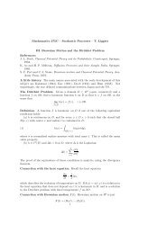
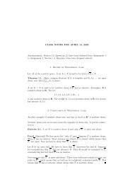
Figure 7.1: The setting of Cantor-Schröder-Bernstein Theorem: f maps X injectively
onto B ⇢ Y and g maps Y injectively onto A ⇢ X. The shaded oval inside A
indicates the result of infinite iteration of g f on X, i.e., the set T
n 1(g f ) n (X).
This set is invariant under g f which, in fact, acts bijectively on it.
f
g
B
Y

4 CHAPTER 7. INFINITE PRODUCT SPACES
h is an identity, while in the first case we note that g h is the bijection g h : (g
f ) n (A \ C) ! (g f ) n+1 (A \ C). Hence g h maps X bijectively onto
⇣ [
(g f ) n ⌘ ✓ ⇣ [
(X \ A) [ (g f ) n ⌘
(A \ C) [ \
(g f ) n ◆
(X) = A. (7.7)
n 1
n 0
Since all of these maps are measurable, so is the above partition of A. It follows
that h is measurable too.
The crux of the above theorem is that we only need to demonstrate the existence
of Borel isomorphism(s) onto subsets of the relevant spaces. We will eventually use
open, continuous bijections, i.e., homeomorphisms. Here it is important to characterize
the image of a Polish space under a homeomorphism. Recall that a Gd is a class
of sets in a topological space that are countable intersections of open sets.
Lemma 7.4 Let X and Y be Polish and let g : X ! B ⇢ Y be a homeomorphism—i.e., a
bijection that is open and continuous. Then B is a Gd subset of Y.
Proof. Let f = g 1 : B ! X. Define the oscilation of f by
n 0
osc f (y) =inf diamX( f (U)): U 3 y open . (7.8)
(This is defined at all y 2 Y.) Suppose y 2 ∂B is such that osc f (y) = 0. Then
for any yn ! y, yn 2 B, xn = f (yn) converges to x = limn!• f (yn). Since X is
complete, we have x 2 X and so y = limn!• yn = limn!• g(xn) =g(x). It follows
that y 2 B, i.e.,
B = B \ y 2 Y : osc f (y) =0 . (7.9)
But closed sets are Gd in metric spaces and {osc f = 0} is Gd because
{osc f = 0} = \
n 1
{osc f < 1/ n} (7.10)
and because osc f is upper semicontinuous, non-negative and so continuous on {osc f =
0}. Hence B is also a Gd set.
The actual use of Theorem 7.3 is enabled by the following observation:
Lemma 7.5 The spaces [0, 1], C =[0, 1] N , N = N N and [0, 1] N , equipped with their
natural Polish topologies, are Borel isomorphic.
Proof. This results from the string of open, continuous (and thus Borel) injections:
[0, 1] ,! C ,! N ,! [0, 1] N ,! [0, 1] (7.11)
The first map is the injection defined by writing each number in [0, 1] in dyadic
form. The second map is a simple inclusion. The third map is induced by the
continued fraction expansion: if x 2 [0, 1] \ Q, there exists a unique sequence (an) 2
{0, 1, . . . } N such that
1
x =
(7.12)
1
a1 +
a2 + 1
a3+...

7.2. PROOF OF BOREL ISOMORPHISM THEOREM 5
1
and noting that, since an = b x c, if x is irrational two distinct sequences will
an 1
lead to two distinct numbers. The fourth injection is a diagonal map: Write an
element x =(x1, x2,...) 2 [0, 1] N by means of a matrix am,n 2{0, 1} such that
Now consider the diagonal map
xm = Â n 1
k 1
f(x) =Â Â
k 1 m=1
am,n
, m 1. (7.13)
2n a m,m k
. (7.14)
21+···+k 2+m
It is easy to check that this map is continuous, one-to-one and the inverse is continuous.
By Lemma 7.4, the images of these maps are Borel and so all maps are Borel
measurable. By Theorem 7.3, all of these spaces are Borel isomorphic.
Recall the well-known fact—which enables the definition of dimension—that [0, 1]
and [0, 1] 2 are not homeomorphic. However, by the arguments in the above lemma,
as standard Borel spaces they are indistinguishable.
Having proved the Borel-equivalence of examples 2-4 in our list above, let us now
address the embedding of a general Polish space. Here it is convenient to work
with Hilbert cube:
Proposition 7.6 [Universality of Hilbert cube] Every Polish space is homeomorphic
to a Gd-subset of [0, 1] N .
Proof. Let (X, d) be a Polish space and let us assume without loss of generality
that d 1 (otherwise maps (X, d) ! (X, d
1+d ) by identity map). Let (xn) be a
countable dense set in X. Define the map f : X ! [0, 1] N by
x 2 X 7! f (x) = d(x, xn) n 1 2 [0, 1] N . (7.15)
As is easy to check, f is continuous and one-to-one and so we have f 1 : f (X) ! X.
We claim that f 1 is also continuous. Indeed, suppose that (zn) is a sequence such
that f (zn) ! f (z) in f (X). Let e > 0 and find n 1 such that d(xn, z) < e. Then
d(zm, z) apple d(zm, xn)+d(xn, z)
= f (zm)n + d(z, xn) !
n!• f (z)n + d(z, xn) < 2e. (7.16)
Hence zm ! z or, in explicit terms, f 1 ( f (zm)) ! f 1 ( f (z)), and so f 1 is continuous
on f (X). Thus f : X ! f (X) is a homeomorphism and so, by Lemma 7.4, f (X)
is a Gd subset of [0, 1] N .
The previous proposition gives the desired embedding of X into the Hilbert cube
and, by Lemma 7.5, a Borel isomorphism into the Cantor space. It remains to construct
an embedding of the Cantor space into a general (uncountable) Polish space.

6 CHAPTER 7. INFINITE PRODUCT SPACES
Theorem 7.7 [Cantor-Bendixon] Let X be a second countable topological space (i.e.,
with countable basis of the topology). Then there exists unique subsets P and O with P
perfect (i.e., having no isolated points) and O countable open such that
X = P [ O and P \ O = ∆. (7.17)
Proof. Let {Un} be a countable basis (of open sets) and let
O = [ Un : Un countable . (7.18)
Then O is open and countable while P = X \ O is closed. Let x 2 P. If U 3 x is open,
then U—being the union of a subcollection from {Un} is necessarily uncountable,
because otherwise x would end up in O. This means that P \ U \{x} 6= ∆, i.e., x is
not isolated.
If P 0 and O 0 are two other such sets, then U \ P 0 6= ∆ implies that U \ P 0 is uncountable,
for any U open. Hence P 0 \ O = ∆, i.e., P 0 ⇢ P. On the other hand, O 0 is countable
open and so it appears in the union defining O. Hence O 0 ⇢ O. If P 0 [ O 0 = X,
then we must have P 0 = P and O 0 = O.
The relevant consequence of this general theorem is as follows:
Corollary 7.8 [Cantor space to Polish space] Every uncountable Polish space contains
a homeomorphic copy of C (and so it has cardinality 2 @0).
Proof. Let X be an uncountable Polish space. Every separable metric space is second
countable, so let X = P \ O be as in the previous theorem. Then P—being a closed
subset of X—is Polish too, so we may as well assume that X = P. We will use the
standard “tree-like” construction to identify a copy of C in X.
Let (xn) be a countable dense set (of distinct points) in P. As is easily checked, there
exist two functions f0 and f1 from {x1,...} to itself such that
and
max d( f0(xn)), xn), d( f1(xn)), xn) apple 2 n
min d( f0(xn)), xn), d( f1(xn)), xn)
(7.19)
d f0(xn), f1(xn) > 0. (7.20)
We now define a collection of balls Bs, indexed by s{0, 1} n , centered at points
of {x1, x2,...} as follows: Set B? to ball of radius 1/ 2 about x1. If Bs is defined
for all s{0, 1} n , and ˜xs are their centers, let rn be the minimum of f0( ˜xs) and f1( ˜xs)
for all s 2{0, 1} n . Then let Bs0 be the ball centered at f0( ˜xs) of radius rn
4 , and
similarly let Bs1 be the corresponding ball centered at f1( ˜xs). These balls are disjoint
with Bs0, Bs1 ⇢ Bs and, by induction, the same is true for {Bs : s{0, 1} n } for
all n 1.
Now let s =(s1, s2,...) 2{0, 1} N . By construction, the intersection T
n 1 B (s1,...,sn)
is non-empty and, by the completeness of X, it contains exactly one point ys.
Moreover, if s and ˜s agree in the first n digits and sn+1 = 0 and s0 then ys 2 B (s1,...,sn,0) and y ˜s 2 B (s1,...,sn,1) and so
n+1 = 1,
rn
2 apple d(ys, y ˜s) apple 2 n
(7.21)

7.3. PRODUCT MEASURE SPACES 7
Thus the map s 7! yn is one-to-one and continuous. To show that the inverse
map is continuous, let us note that if d(ys, y ˜s) < e, then sn = s 0 n for all n for
which rn/ 2 > e. So the smaller e, the larger part of s and ˜s must be the same.
Hence, the inverse map is continuous.
Now we are finally ready to put all pieces together:
Proof of Theorem 7.2. If X is finite or countable, then the desired Borel isomorphism
is constructed directly. So let us assume that X is uncountable. Then Corollary 7.8
says there is a homeomorphism C ,! X while Proposition 7.6 says there exists a
homeomorphism X ,! [0, 1] N . Both of these image into a Gd-set by Lemma 7.4
and so the inverse is Borel measurable. Since [0, 1] N is Borel isomorphic to [0, 1] N ,
we thus we have Borel-embeddings C ,! X and X ,! C . From Theorem 7.3 it
follows that X is Borel isomorphic to C —and thus to any of the spaces listed in
Lemma 7.5.
7.3 Product measure spaces
Definition 7.9 [General product spaces] Let (Wa, Fa)a2I be any collection of measurable
spaces. Then W = ⇥a2I Wa can be equipped with the product s-algebra F =
N
a2I Fa which is defined by
✓n o
F = s ⇥ Aa : Aa 2 Fa &#{a 2I: Aa 6= Wa} < •
a2I
◆
. (7.22)
If Wa = W0 and Fa = F0 then we write W = W I 0
and F = F ⌦I
0 .
Next we note that standard Borel spaces behave well under taking countable products:
Lemma 7.10 Let I be a finite or countably infinite set and let (Wa, Fa)a2I be a family
of standard Borel spaces. Let (W, F ) be the product measure space defined above. Then
(W, F ) is also standard Borel. Moreover, if fa : Wa ! [0, 1] are Borel isomorphisms, then
f = ⇥a2I fa is a Borel isomorphism of W onto [0, 1] I .
Our goal is to show the existence of product measures. We begin with finite products.
The following is a restatement of Lemma 4.13:
Theorem 7.11 Let (W1, F1, µ1) and (W2, F2, µ2) be probability spaces. Then there
exists a unique probability measure µ1 ⇥ µ2 on F1 ⌦ F2 such that for all A1 2 F1,
A2 2 F2,
µ1 ⇥ µ2(A1 ⇥ A2) =µ1(A1)µ2(A2). (7.23)
The reason why this is not a trivial application of Carathéodory’s extension theorem
is the fact that (7.26) defines µ1 ⇥ µ2 only on a structure called semialgebra and
not algebra.
Definition 7.12 A non-empty collection S ⇢ P(W) is called semialgebra if

8 CHAPTER 7. INFINITE PRODUCT SPACES
(1) A, B 2 S implies A \ B 2 S .
(2) If A 2 S , then there exist Ai 2 S disjoint such that A c = S n i=1 Ai.
It is easy to verify that semialgebras on W automatically contain W and ∆.
Lemma 7.13 The following are semialgebras:
(1) S = {(a, b] : • apple a apple b apple •}
(2) S = {A1 ⇥···⇥An : Ai 2 Ai} where Ai are algebras.
(3) S = ⇥ Aa : Aa 2 Aa &#{a : Aa 6= Wa} < • provided Aa’s are algebras.
a2I
Proof. Let us focus on (2): Since all Ai are p-systems, S is closed under intersections.
To show the complementation property in the definition of semialgebra,
let D be a collection of all sets of the form B1 ⇥···⇥Bn, where Bi is either Ai or A c i ,
but such that A1 ⇥···⇥An is not included in D. Then
(A1 ⇥···⇥An) c = [
From here the complementation property follows by noting that D is finite and
D ⇢ S .
Next we will show that via finite disjoint unions semialgebras give rise to algebras:
Lemma 7.14 Let S be a semialgebra and let S be the set of finite unions of sets Ai 2 S .
Then S is an algebra.
Proof. First we show that S is closed under intersections. Indeed, A is the (finite)
union of some Ai 2 S and B is the (finite) union of some Bj 2 S . Therefore,
✓
[
A \ B =
i
Ai
◆
\
B2B
B.
✓ ◆
[
Bj =
j
[
Ai \ Bj.
i,j
Since Ai, Bj 2 S , then Ai \ Bj 2 S and A \ B is the finite union of sets from S .
Consequently, A \ B 2 S .
Next we will show that S is closed under taking the complement. Let A be as
above. Then
A c ✓
[
=
◆c = \ \ [
= Bi,j,
i
Ai
where Bi,j 2 S are such that A c i is the union of Bi,j—see the definition of semialgebra.
The union on the extreme right is finite and, therefore, it belongs to S . But
S is closed under finite intersections, so A c 2 S as well.
Now we will learn how (and under what conditions) a set function on a semialgebra
can be extended to a measure on the associated algebra:
i
A c i
i
j

7.3. PRODUCT MEASURE SPACES 9
Theorem 7.15 Let S be a semialgebra and let µ : S ! [0, 1] be a set function. Suppose
the properties hold:
(1) Finite additivity: A, Ai 2 S ,A= S n i=1 Ai disjoint ) µ(A) =Â n i=1 µ(Ai),
(2) Countable subadditivity: A, Ai 2 S ,A= S • i=1 Ai disjoint ) µ(A) apple  • i=1 µ(Ai).
Then there exists a unique extension ¯µ : S ! [0, 1] of µ, which is a measure on S .
Proof. Note that (1) immediately implies that µ(∆) =0. The proof comes in four
steps:
Definition of ¯µ: For A 2 S , then A = S n i=1 Si for some Si 2 S . Then we let
¯µ(A) = n i=1 µ(Si). This definition does not depend on the representation of A;
if A = S m j=1 Ti for some Tj 2 S , then the fact that S is a p-system and finite
additivity of µ ensure that
n
 µ(Si) =
i=1
n ⇣ [ m ⌘
 µ Si \ Tj =
i=1 j=1
n m
 Â
i=1 j=1
µ(Si \ Tj) =
m
 µ(Tj).
j=1
Finite additivity of ¯µ: By the very definition, ¯µ is also finitely additive, because if
An is given as the disjoint union S
i Si,n, then S
n An = S
i,n Si,n and thus ¯µ( S
n An) =
Âi,n µ(Si,n) =Ân ¯µ(An). (All indices are finite.)
Countable subadditivity of ¯µ: We claim that ¯µ is countably subadditive, whenever
the disjoint union lies in S . Let Ai 2 S and A = S
k 1 Ak 2 S . Writing Ak =
S
n Sj—note the efficient way to index the Sj’s contributing to A kapplejn Ak is also in S
because S is an algebra. Since we already showed that ¯µ is finitely additive, we
have
n
¯µ(A) = ¯µ(Bn)+  ¯µ(A k)
n
 ¯µ(A k).
k=1
k=1
Letting n ! •, the opposite inequality follows.

10 CHAPTER 7. INFINITE PRODUCT SPACES
Thus we have a well defined function ¯µ : S ! [0, 1] which is finitely additive
on S and countably additive on disjoint unions that belong to S . These are the
properties required to be a measure on an algebra.
Note that the combination of Lemma 7.13, Lemma 7.14 and the construction of
the measure ¯µ from Theorem 7.15 provide an alternative proof of the fact that
Lebesgue-Stieltjes measures on R are defined by the corresponding “distribution”
function.
Proof of Theorem 7.11. The set S = {A1 ⇥ A2 : Ai 2 Fi} is a semialgebra by
Lemma 7.13 and s(S ) is the product s-algebra F1 ⌦ F2. We will show that the set
function µ : S ! [0, 1] defined by
µ(A1 ⇥ A2) =µ1(A1)µ2(A2), Ai 2 Fi,
is countably additive on S —this implies the desired properties (1-2) in Theorem 7.15.
Let A 2 F1 and B 2 F2 and suppose that A ⇥ B is the disjoint union S
j Aj ⇥ Bj,
where Aj 2 F1 and Bj 2 F2, and where j is either finite or countable index. The
proof uses integration: For each x 2 A, let I(x) ={j : Aj 3 x}. Now since {x}⇥
Bj ⇢ Aj ⇥ Bj whenever j 2I(x), the sets {x}⇥Bj with j 2I(x) are disjoint and
{x}⇥ S
j2I(x) Bj = {x}⇥B. It follows that B is the disjoint union
and thus
B = [
1A(x)µ2(B) =Â j
j2I(x)
Bj
1A j (x)µ2(Bj)
for any x 2 W1. Both sides are F1-measurable, and integrating with respect to µ1
we get
µ1(A)µ2(B) =Â µ1(Aj)µ2(Bj).
j
This shows that µ(A ⇥ B) equals the sum of µ(Aj ⇥ Bj) and so µ is countably additive.
Lemma 7.14, Theorem 7.15 and Carathéodory’s extension theorem then guarantee
that µ has a unique extension to F1 ⌦ F2.
General finite product spaces are handled by induction using the fact that
nO ⇣nO 1 ⌘
Fi = Fi ⌦ Fn
i=1 i=1
Note that this proves the associativity of the product of measures:
We leave the details of these calculations implicit.
(7.24)
(µ1 ⇥ µ2) ⇥ µ3 = µ1 ⇥ (µ2 ⇥ µ3). (7.25)

7.4. KOMOGOROV’S EXTENSION THEOREM 11
7.4 Komogorov’s extension theorem
We now address the corresponding extension of measures to infinite product spaces:
Theorem 7.16 [Kolmogorov’s extension theorem] Let M be a compact metric space,
B = B(M) the Borel s-algebra on M and, for each n 1, let µn be a probability measure
on (M n , B ⌦n ). We suppose these measures are consistent in the following sense:
8n 1, 8A1,...,An 2 B : µn+1(A1 ⇥···⇥An ⇥ M) =µn(A1 ⇥···⇥An).
Then there exists a unique probability measure µ on (M N , B ⌦N ) such that
µ(A1 ⇥···⇥An ⇥ R ⇥ R ...)=µn(A1 ⇥···⇥An) (7.26)
holds for any n 1 and any Borel sets Ai 2R.
As many extension arguments from measure theory, the proof boils down to proving
that if a sequence of sets decreases to an empty set, then the measures decrease
to zero. In our case this will be ensure through the following lemma:
Lemma 7.17 Let W be a metric space and let A be an algebra of subsets of W (which is
not necessarily a s-algebra). Suppose that µ : A ! [0, 1] is a finitely-additive set function
which is regular in the following sense: For each set B 2 A and each e > 0, there exists a
compact set C 2 A such that
C ⇢ B (7.27)
and
µ(B \ C) apple e. (7.28)
Then for each decreasing sequence Bn 2 A with Bn # ∆ we have µ(Bn) # 0.
Proof. Let Bn be a decreasing sequence of sets with limn!• µ(Bn) =d > 0. We will
show that T
n Bn 6= ∆. By the assumptions, we can find compact sets Cn 2 A such
that Cn ⇢ Bn and µ(Bn \ Cn) < d2 n 1 . Now since Bn Bn+1, we have
Bn \
n[
(Bk \ Ck) ⇢
k=1
n\
Ck. Indeed, if x 2 Bn then x 2 B k for all k apple n and then x can only belong to the set on
the left if x 2 C k for all k apple n. Using finite additivity of µ, it follows that
⇣ \ n
µ
k=1
C k
⌘
µ(Bn)
k=1
n
 µ(Bk \ Ck) d  µ(Bk \ Ck) k=1
k 1
Consequently, since finite additivity implies that µ(∆) =0, the intersection T n k=1 C k
is non-empty for any finite n. But the sets Cn are compact and thus T • k=1 C k 6= ∆.
The inclusions Cn ⇢ Bn imply that also T
n Bn 6= ∆.
Lemma 7.17 links measure with topology (which is the reason why we often consider
standard Borel spaces). Next we observe:
d
2 .

12 CHAPTER 7. INFINITE PRODUCT SPACES
Lemma 7.18 Let (M, r) be a compact metric space. Equip M N with the metric
d(x, y) =Â r(xn, yn)2
n 1
n
(7.29)
whenever x =(xn) 2 M N and y =(yn) 2 M N . Then (M N , d) is a compact metric
space. Moreover, if C1,...,Cn are compact sets in (M, r), then C1 ⇥···⇥Cn ⇥ M ⇥
M ⇥··· is compact in (M N , d).
Proof. The first part is a reformulation of Tychonoff’s theorem for product spaces.
The second part is checked directly.
Now we are finally ready to prove Kolmogorov’s theorem:
Proof of Theorem 7.16. Consider the set
S = A1 ⇥···An ⇥ M ⇥···: Ai compact in M 8i
Then, as is easy to check, S is a semialgebra. Let µ : S ! [0, 1] be defined by
(7.30)
µ(A1 ⇥···⇥An ⇥ M ⇥···)=µn(A1 ⇥···⇥An) (7.31)
The consistency condition for µn shows that this gives the same number regardless
of the representation of the set A1 ⇥···⇥An ⇥ M ⇥···. Let S be the set of all
finite disjoint unions of elements from S . By Lemma 7.14, S is an algebra; we
extend µ to a set function ¯µ : S ! [0, 1] by additivity. A similar argument to that
used in the proof of Theorem 7.15 now shows that ¯µ is well-defined and finitely
additive.
It remains to show that ¯µ is countably additive. To that end, let A1, A2, ···2S be
disjoint with A = S
n 1 An 2 S . Define DN = S
n>N An and note that DN 2 S as
well. Then A1,...,An, Bn are disjoint and so finite additivity of ¯µ implies
¯µ(A) = ¯µ(A1)+···+ ¯µ(An)+ ¯µ(Dn) (7.32)
We thus need to show that ¯µ(Dn) ! 0 as n ! •. Here we use the topology: By
Lemma 7.17 it suffices to show
8e > 0 8B 2 S 9C 2 S : C ⇢ B compact & ¯µ(B \ C) < e. (7.33)
But B 2 S is a finite disjoint union of Bi 2 S and so it clearly suffices to prove
this for B 2 S . However, every B 2 S is compact by Lemma 7.18 and so we
can take C = B above and the regularity property holds trivially. By Lemma 7.17,
we have ¯µ(Dn) ! 0 and ¯µ is thus countably additive on S . The Carathéodory
extension theorem now implies the existence of a unique extension of ¯µ to s(S )=
B ⌦N .
The proof in the textbook bundles Lemma 7.17 with the proof of Tychonoff’s theorem.
We prefer to separate these to highlight the role of Borel regularity (Lemma 7.17)
which is a property of separate interest. Note also that the consistency condition
holds only for probability; extensions of other measures are not meaningful. In
fact, it is known that one cannot construct an infinite product of Lebesgue measures
on R.

7.5. TWO ZERO-ONE LAWS 13
7.5 Two zero-one laws
We will demonstrate the usefulness of the infinite product spaces by proving two
Zero-One Laws. We demonstrate these on an example of percolation.
Example 7.19 Percolation : Let p 2 [0, 1] and let B denote the set of edges of Z d .
(We regard the latter as a graph with vertices at points of R d with integer coordinates
and edges between any two points with Euclidean distance one.) Let (h b) b2B
be i.i.d. Bernoulli(p). We may view each h =(h b) as a subgraph of (Z d , B)—with
edge set {b 2 B : h b = 1}. The question is: Does this graph have an infinite connected
component? We define
E• = {h : h has an infinite connected component}. (7.34)
We refer to edges with h b = 1 as occupied and those with h b = 0 as vacant. To set
the notation, we will denote by Pp the law of h with parameter p.
First we have to check that E• is an event:
Lemma 7.20 E• is measurable (w.r.t. the product s-algebra on {0, 1} B ).
Proof. Let F denote the product s-algebra on {0, 1} B . We have to show E• 2 F .
For each n 1 and each x 2 Z d , consider the event
En(x) = x connected to (x +[ n, n] d ) c in h
(7.35)
that x is connected by a path of occupied edges to the boundary of a box of side 2n
centered at x. Since En(x) depends only on a finite number of hb’s, it is measurable.
But
E• = \ [
En(x) (7.36)
and so E• 2 F as well.
n 1 x2Zd Next we observe that E• does not depend on the status on any given finite number
of edges. Indeed, if an edge is occupied, making it vacant may increase the number
of infinite component but it won’t destroy them while. Similarly, making a vacant
edge occupied may connect two infinite components together but if there is none,
it will not create one. In a more technical language, E• is a tail event according to
the following definition:
Definition 7.21 Let X1, X2,... be random variables. Then T = T
n 1 s(Xn, Xn+1,...)
is the tail s-algebra and events from T are called tail events.
Here is our first zero-one law:
Theorem 7.22 [Komogorov’s Zero-One Law] Let X1, X2,... be independent and let
T = T
n 1 s(Xn, Xn+1,...) be the tail s-algebra. Then
8A 2 T : P(A) 2{0, 1}. (7.37)

14 CHAPTER 7. INFINITE PRODUCT SPACES
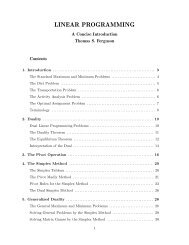
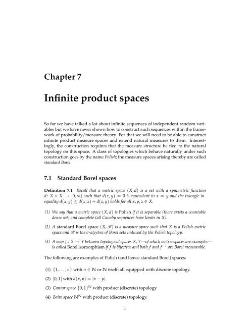
Figure 7.2: The infinite connected component in 40⇥40 box centered at the origin
for percolation with parameter p = 0.55. The finite components are not depicted.
Proof. We will show that T is independent of F . First pick n 1 and note
A 2 s(X1,...,Xn) & B 2 s(Xn+1, Xn+2,...) ) A, B independent (7.38)
But T ⇢ s(Xn+1, Xn+2,...) and so
A 2 s(X1,...,Xn) & B 2 T ) A, B independent (7.39)
This now holds for all n 1 and so
A 2 [
s(X1,...,Xn) & B 2 T ) A, B independent (7.40)
n 1
But S
n 1 s(X1,...,Xn) is a p-system and F = s( S
n 1 s(X1,...,Xn)) and so Theorem
4.6 implies
A 2 F & B 2 T ) A, B independent (7.41)
Let now A 2 T . Then A is independent of itself which yields
This permits only P(A) =0 or P(A) =1.
Here is a consequence of this law for percolation:
P(A) =P(A \ A) =P(A) 2 . (7.42)

7.5. TWO ZERO-ONE LAWS 15
Corollary 7.23 For each d 1 there exists pc 2 [0, 1] such that
(
0, if p < pc,
Pp(E•) =
1, if p > pc,
At p = pc we have Ppc(E•) 2{0, 1}.
(7.43)
Proof. We have already shown that E• 2 T and so Pp(E•) 2{0, 1} for all p. It
is also clear that the larger p the more edges there are and so Pp(E•) should be
increasing. However, to prove this we have to work a bit.
The key idea is that we can actually realize percolation for all p’s on the same probability
space. Consider i.i.d. random variables U =(U b) b2B whose law is uniform
on [0, 1] and define
h (p)
b = 1 {U bapplep}. (7.44)
Clearly, h (p) =(h (p)
b ) are i.i.d. Bernoulli(p) so they realize a sample of percolation at
parameter p. Now let E•(p) ={U : h (p) contains infinite connected component}.
Since p 7! h (p)
b increases, if E•(p) occurs, then so does E•(p 0 ) for p0 > p. In other
words
p 0 > p ) E•(p) ⇢ E•(p 0 ) (7.45)
This implies
Pp(E•) =P E•(p) apple P E•(p 0 ) = P p 0(E•), (7.46)
i.e., p 7! Pp(E•) is non-decreasing. Since it takes values zero or one, there exists a
unique point where Pp(E•) jumps from zero to one. This defines pc.
Let us remark what really happens: It is known that
(
= 1, d = 1,
pc
2 (0, 1), d 2.
(7.47)
At d = 2 it is known that pc = 2 (Kesten’s Theorem) but the values for d 3
are not known explicitly (and presumably are not of any special form). Concerning
Ppc(E•), it is widely believed that this probability is zero—there is no infinite
cluster at the critical point—but the proof exists only in d = 2 and d 19.
Our next object of interest is the random variable:
N = number of infinite connected components in h (7.48)
The values N can take are {0, 1, . . . }[{•}. The random variable N definitely
depends on any finite number of edges and so N is not T -measurable. (The reason
why we care is if it were tail measurable then it would have to be constant a.s.)
However, N is clearly translation invariant in the following sense:
Definition 7.24 Let tx : {0, 1} B !{0, 1} B be the map defined by
(txh) b = h b+x
(7.49)
We call tx the translation by x. An event A is translation invariant if t 1
x (A) =A for
all x 2 Z d . A random variable N is translation invariant if N tx = N.

16 CHAPTER 7. INFINITE PRODUCT SPACES
First we note that the measure Pp is translation invariant:
Lemma 7.25 Let Pp be the law of Bernoulli(p) on B. Then Pp is translation invariant,
i.e., P t 1
x = Pp for all x 2 Z d .
Proof. This is verified similarly as translation invariance of the Lebesgue measure.
First, a direct calculation shows that Pp(t 1
x (A)) = Pp(A) for all cylinder events.
But the class of sets in F satisfying this identity is a l-system, and since cylinder
sets form a p-system, we have invariance of Pp on the s-algebra generated by
cylinder events. This is all of F .
Next we will prove that every translation invariant event in F is a zero-one event:
Theorem 7.26 [Ergodicity of i.i.d. measures] Let (Xn)n2Z be i.i.d. and let t be the
left-shift acting on the sequence (Xn) via
Then
t(··· , X 1, X0, X1, ···)=(··· , X0, X1, X2, ···). (7.50)
8A 2 s(Xn : n 2 Z) : t 1 (A) =A ) P(A) 2{0, 1}. (7.51)
Proof. We proceed in a way similar to Komogorov’s law; the goal is to show that a
translation invariant set is independent of itself. However, since not all translation
invariant events are tail events, we have use approximation to derive the result.
Let F = s(Xn : n 2 Z), Fn = s(X n, ··· , Xn) and let A 2 F be of positive
measure. The construction of Carathéodory extension of the measure to F shows
that there exists a sequence An 2 Fn such that An approximates A in the sense
P(A4An) !
n!• 0, (7.52)
where A4An denotes symmetric difference. Suppose now that t 1 (A) =A and
recall that P is t-invariant. This means that t 1 (An) approximates t 1 (A) as well
as An,
P (A4t 1 (An) = P(A4An). (7.53)
Iterating this 2n + 1 times we get a set t (2n+1) (An) which is in s(X 3n 1,...,X n 1)
and is thus independent of An. Thus, we may approximate A equally well by two
disjoint sets An and t (2n+1) (An).
Now we will derive the independence of A of itself: The key will be the identity
P(A \ B) apple P(C \ D)+P(A4C)+P(B4D) (7.54)
which we will apply to B = A, C = An and D = t (2n+1) (An). This yields
P(A) =P(A \ A) apple P An \ t (2n+1) (An) + P(A4An)+P A4t (2n+1) (An) .
(7.55)
Since An and t (2n+1) (An) are independent have equal probability, (7.53) gives us
P(A) apple P(An) 2 + 2P(A4An). (7.56)

7.5. TWO ZERO-ONE LAWS 17
However P(An) apple P(A)+P(A4An) and so (7.52) gives
This is only possible if P(A) =0 or P(A) =1.
P(A) apple P(A) 2 . (7.57)
Going back to percolation, the above zero-one law tells us:
Corollary 7.27 One of the events {N = 0}, {N = 1}, and {N = •} has probability
one.
Proof. All of these events are translation invariant (or tail) and so they have probability
zero or one. We have to show that P(N = k) =0 for all k 2{2, 3, . . . }. Again,
if this is not the case then P(N = k) =1 because {N = k} is translation invariant;
for simplicity let us focus on k = 2. If P(N = 2) =1 then there exists n 1 such
that the event
( )
d
box [ n, n] is connected to infinity by two disjoint paths that are
Cn =
not connected to each other in the complement of the box [ n, n] d
(7.58)
occurs with probability at least 1/ 2. Indeed, {N = 2} ⇢ S
n 1 Cn and Cn is increasing.
However, the event Cn is independent of the edges inside the box [ n, n] d and
so with positive probability, the two disjoint paths get connected inside the box.
This means that N = 1 with positive probability on the event {N = 2}\Cn, i.e.,
P(N = 1) > 0. This contradicts P(N = 2) =1.
Let us conclude by stating what really happens: we have P(N = •) =0 so we
either have no infinite cluster or one infinite cluster a.s. The most beautiful version
of this argument comes in a theorem of Burton and Keane which combines rather
soft arguments not dissimilar to what we have seen throughout this section.