1.72, Groundwater Hydrology Prof. Charles Harvey Lecture Packet #3

1.72, Groundwater Hydrology
Prof. Charles Harvey
Lecture Packet #3: Hydraulic Head and Fluid Potential
What makes water flow?
Consider pressure
Water Level
C
po
Pressure at A = atmospheric (po)
Pressure at B > atmospheric (po + ∆p)
Pressure at C = atmospheric (po)
But flow is not from A to B to C.
Flow is not “down pressure gradient.”
Hubbert (1940) – Potential
po
po + ∆p
A
Water Level
A physical quantity capable of measurement at every point in a flow system,
whose properties are such that flow always occurs from regions in which the
quantity has less higher values to those in which it has lower values
regardless of the direction in space.
Examples:
Heat conducts from high temperature to low temperature
• Temperature is a potential
Electricity flows from high voltage to low voltage
• Voltage is a potential
Fluid potential and hydraulic head
Fluids flow from high to low fluid potential
• Flow direction is away from location where mechanical energy per unit mass
of fluid is high to where it is low.
• How does this relate to measurable quantity?
1.72, Groundwater Hydrology Lecture Packet 3
Prof. Charles Harvey Page 1 of 9
B

Groundwater flow is a mechanical process – forces driving fluid must overcome
frictional forces between porous media and fluid. (generates thermal energy)
Work – mechanical energy per unit mass required to move a fluid from point z to
point z’.
Elevation: z’
Pressure: p
Velocity: v
Density: ρ
Volume: V
Elevation: z=0
Pressure: p=po
Velocity: vo
Density: ρo
Volume: Vo
z’
z
Fluid potential
is mechanical
energy per unit
mass = work
to move unit
mass
1.72, Groundwater Hydrology Lecture Packet 3
Prof. Charles Harvey Page 2 of 9

Which way does water flow (function of Z and P) ?
hp1
z1
hp1
z1
Q
Q
hp2
z2
hp2
z2
Fluid potential is the mechanical energy per unit mass of fluid potential at z’ = fluid
potential at datum + work from z to z’.
The work to move a unit mass of water has three components:
1) Work to lift the mass (where z = 0)
w 2 = mgz'
2) Work to accelerate fluid from v=0 to v’
w 2
=
2
mv
2
hp1
hp1
3) Work to raise fluid pressure from p=po to p
p p p
z1
V dp
w3 = ∫Vdp = m∫ dp = m∫ m p
po po po
1.72, Groundwater Hydrology Lecture Packet 3
Prof. Charles Harvey Page 3 of 9
z1
Q
Q
hp2
z2
hp2
z2

Note that a unit mass of fluid occupies a volume V = 1/ρ
The Fluid Potential (the mechanical energy per unit mass, m=1)
φ = gz + v + ∫ dp +
2 p
p o
2
φ = gz + v
2 +
2
p
p −
p
p
0
for incompressible fluid (ρ is constant)
This term is almost always unimportant in groundwater
flow, with the possible exception of where the flow is very
fast, and Darcy’s Law begins to break down.
How does potential relate to the level in a pipe?
At a measurement point pressure is described by:
P = ρ g(depth) + po
p = ρ gϕ + po
p = ρ g(h-z) + po
Return to fluid potential equation
2
− 0
φ = gz + v p p
+
2 p
Neglect velocity (kinetic) term, and substitute for p
So,
ρ g ( h − z ) + 0
φ = gz +
ρ
p − 0 p
φ = gh or h = φ / g
Thus, head h is a fluid potential.
1.72, Groundwater Hydrology Lecture Packet 3
Prof. Charles Harvey Page 4 of 9
ϕ
z
h

• Flow is always from high h to low h.
• H is energy per unit weight.
• H is directly measurable, the height of water above some point.
Thermal Potential
h = z + ϕ
ϕt = Thermal Potential
Temperature can be an important driving force for groundwater and soil moisture.
• Volcanic regions
• Deep groundwater
• Nuclear waste disposal
Can cause heat flow and also drive water.
Chemical Potential
Adsorption Potential
Total Potential is the sum of these, but for saturated conditions for our initial cases
we will have:
*
q = − L1
ϕ = ϕg + ϕp
∂ h ∂ T
− L2
∂ l ∂ l
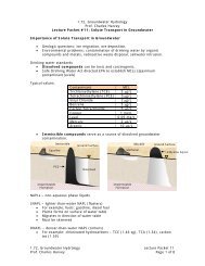
Derivation of the Groundwater Flow Equation
Darcy’s Law in 3D
Homogeneous vs. Heterogeneous
Isotropic vs. Anisotropic
L
− 3
Isotropy – Having the same value in all directions. K is a scalar.
K
∂ c
∂ l
h
∂h ∂ h
K
x
∂y ∂ z
∂
= −
= − K = − K
∂
q x q y q z
Anisotropic – having directional properties. K is really a tensor in 3D
Gradient
K
Flow
The value that converts one vector to another vector is a tensor.
1.72, Groundwater Hydrology Lecture Packet 3
Prof. Charles Harvey Page 5 of 9

y
q = − K ∂ h ∂ h
xx − K xy
∂ x ∂ y − K ∂ h
x
xz
∂ z
q y = − K yx
∂ h ∂ h ∂ h
− K yy − K yz
∂ x ∂ y ∂ z
∂h ∂h
∂ h
= − K − K − K zz
∂x ∂y
∂ z
qz zx zy
• The first index is the direction of flow
• The second index is the gradient direction
Interpretation - Kxx is a coefficient along the x-direction that contributes a
component of flux along the x-axis due to the coefficient along the z-direction that
contributes a component of flux along the z-axis due to the component of the
gradient in the y-direction.
The conductivity ellipse (anisotropic vs. isotropic)
K yy
Gradient
Flow y
K xx
x
If Kyy = Kxx then the media is isotropic and ellipse is a circle.
It is convenient to describe Darcy’s law as:
q
r = −
K ∇ h
K yy
K xx
Gradient
Flow
Where ∇ is called del and is a gradient operator, so ∇ h is the gradient in all three
directions (in 3D). K is a matrix.
1.72, Groundwater Hydrology Lecture Packet 3
Prof. Charles Harvey Page 6 of 9
x

qx =
qy =
qz =
Kxx Kxy Kxz
Kyx Kyy Kyz
Kzx Kzy Kzz
The magnitudes of K in
conductivities.
Kxx
Kyy
the principal directions
If the coordinate axes are aligned with the principal directions of the conductivity
tensor then the cross-terms drop out giving:
qx =
qy =
qz =
Kzz
∂ h
∂ x
∂ h
∂ y
∂ h
∂ z
∂ h
∂ x
∂ h
∂ y
∂ h
∂ z
are known as the principal
1.72, Groundwater Hydrology Lecture Packet 3
Prof. Charles Harvey Page 7 of 9

Effective Hydraulic Conductivity
Q1
Qtot Q2
Q3
Q4
Qtot = Q1 + Q2 + Q3 + Q4
=
=
=
∆H
L 1 K
∆ x
∆
∆ x
∆ H
∆ x
1
n H
∑
i
L tot K eff
∆Htot
∆H
∆H
∆H
+ L 2 K 2 + L 3 K 3 + L 4K 4
∆ x ∆ x ∆ x
L i K i
∑
i
= n
1.72, Groundwater Hydrology Lecture Packet 3
Prof. Charles Harvey Page 8 of 9
K
eff
n
∑
i
L K
i
L
i
i
Ltot

∆ Htot
∆ Htot = ∆ H1 + ∆ H2 + ∆ H3 + ∆ H4
Q
∆ H1
∆ H2
∆ H3
∆ H4
∆ H tot ∆ H1 ∆ H 2 ∆ H 3
q = K eff = K1 = K 2 = K 3 =
L
∆ H 4
K 4
tot L1 L2 L3 L4 n qL tot qL i
∑ Li = ∑ i
K eff i K i Keff = n
∑ Li n
i K i
1.72, Groundwater Hydrology Lecture Packet 3
Prof. Charles Harvey Page 9 of 9
Ltot