CoDaPack v2 USER's GUIDE

Authors: Thió-Henestrosa, S. and 

Comas, M. 

CoDaPack v2 USER’s GUIDE 

June 6, 2011

Dr. Santiago Thió-Henestrosa 

Professor Titular d’Universitat (full professor) 

University of Girona 

Dept. of Computer Science and Applied Mathematics 

Campus Montilivi — P-1, E-17071 Girona, Spain 

santiago.thio@udg.edu 

Mr. Marc Comas-Cufí 

Professor Associat (adjunct professor) 

University of Girona 

Dept. of Computer Science and Applied Mathematics 

Campus Montilivi — P-1, E-17071 Girona, Spain 

marc.comas@udg.edu 

V

Preface 

The program CoDaPack v2, together with the present manual, can be downloaded 

for free from the web at 

http://ima.udg.edu/CoDaPack 

There is also available a whole library of subroutines for Matlab, developed 

mainly by John Aitchison, which can be obtained from John Aitchison himself 

or from anybody of the compositional data analysis group at the University of 

Girona (www.udg.edu). Finally, those interested in working with R (or S-plus) 

may either use the full-fledged packages “compositions” van den Boogaart 

et al. (2010) or ”robCompositions” Hron et al. (2010). 

Santiago Thió-Henestrosa and Marc Comas-Cufí 

Girona, June 6, 2011

Contents 

1 Introduction . . . . . . . . . . . . . . . . . . . . . . . . . . . . . . . . . . . . . . . . . . . . . . . 1 

1.1 General considerations . . . . . . . . . . . . . . . . . . . . . . . . . . . . . . . . . . . 1 

2 File Menu . . . . . . . . . . . . . . . . . . . . . . . . . . . . . . . . . . . . . . . . . . . . . . . . . 5 

2.1 General remarks . . . . . . . . . . . . . . . . . . . . . . . . . . . . . . . . . . . . . . . . . 5 

3 Data Menu . . . . . . . . . . . . . . . . . . . . . . . . . . . . . . . . . . . . . . . . . . . . . . . . 7 


3.2 Data: Transformations: ALR . . . . . . . . . . . . . . . . . . . . . . . . . . . . . . 7 

3.3 Data: Transformations: CLR . . . . . . . . . . . . . . . . . . . . . . . . . . . . . . 8 

3.4 Data: Transformations: ILR . . . . . . . . . . . . . . . . . . . . . . . . . . . . . . . 9 

3.5 Data: Centering . . . . . . . . . . . . . . . . . . . . . . . . . . . . . . . . . . . . . . . . . 11 

3.6 Data: Subcomposition/Closure . . . . . . . . . . . . . . . . . . . . . . . . . . . . 12 

3.7 Data: Amalgamation . . . . . . . . . . . . . . . . . . . . . . . . . . . . . . . . . . . . . 12 

3.8 Data: Perturbation . . . . . . . . . . . . . . . . . . . . . . . . . . . . . . . . . . . . . . 12 

3.9 Data: Power Transformation . . . . . . . . . . . . . . . . . . . . . . . . . . . . . . 13 

3.10 Data: Rounded Zero Replacement . . . . . . . . . . . . . . . . . . . . . . . . . 14 

3.11 Data: Numeric to categorical . . . . . . . . . . . . . . . . . . . . . . . . . . . . . . 15 

3.12 Data: Categoric to numeric . . . . . . . . . . . . . . . . . . . . . . . . . . . . . . . 16 

3.13 Data: Add numeric variables . . . . . . . . . . . . . . . . . . . . . . . . . . . . . . 16 

3.14 Data: Delete variables . . . . . . . . . . . . . . . . . . . . . . . . . . . . . . . . . . . . 16 

4 Statistics Menu . . . . . . . . . . . . . . . . . . . . . . . . . . . . . . . . . . . . . . . . . . . . 17 


4.2 Statistics: Compositional statistics summary . . . . . . . . . . . . . . . . 17 

4.3 Statistics: Classical statistics summary . . . . . . . . . . . . . . . . . . . . . 18 

4.4 Statistics: Additive-Logistic normality test . . . . . . . . . . . . . . . . . . 19 

4.5 Statistics: Atypicality Indices (Fig. 4.7) . . . . . . . . . . . . . . . . . . . . 19

X Contents 

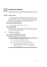
5 Graphs Menu . . . . . . . . . . . . . . . . . . . . . . . . . . . . . . . . . . . . . . . . . . . . . . 23 


5.2 Graphs: Ternary Diagram . . . . . . . . . . . . . . . . . . . . . . . . . . . . . . . . 24 

5.3 Graphs: Principal Components . . . . . . . . . . . . . . . . . . . . . . . . . . . . 24 

5.4 Graphs: ALR Plot . . . . . . . . . . . . . . . . . . . . . . . . . . . . . . . . . . . . . . . 24 

5.5 Graphs: CLR Plot . . . . . . . . . . . . . . . . . . . . . . . . . . . . . . . . . . . . . . . 26 

5.6 Graphs: ILR Plot . . . . . . . . . . . . . . . . . . . . . . . . . . . . . . . . . . . . . . . . 26 

5.7 Graphs: Biplot . . . . . . . . . . . . . . . . . . . . . . . . . . . . . . . . . . . . . . . . . . 27 

5.8 Graphs. Balance Dendrogram . . . . . . . . . . . . . . . . . . . . . . . . . . . . . 27 

References . . . . . . . . . . . . . . . . . . . . . . . . . . . . . . . . . . . . . . . . . . . . . . . . . . . . . 31

1 

Introduction 

The software presented in this manual is still under construction. The idea 

is to build a user-friendly application to be used in all fields of science and 

technology which need to operate with compositional data. It is conceived 

as a complement to other statistical software, which is perfectly appropriate 

for working on coordinates, and not as standalone software for the statistical 

analysis of compositional data. Probably in a future it will incorporate more 

classical statistic features. 

To use this application the Software Java Virtual Machine is needed (minimum 

version 1.5.0). To get it working, it suffices to install and open the file 

CoDaPack.exe. 

CoDaPack v2 is based on menus. Numerical results appear on the output 

part of the window, while graphs appear in new graphical windows. 

1.1 General considerations 

The freeware package can be downloaded from the web site: 

http://ima.udg.edu/CoDaPack. 

The package comes with a setup file and requires having Java Virtual Machine 

(minimum version 1.5.0) installed. When a new version is available, CoDaPack 

v2 shows a message asking for the user to import the new version. 

To use CoDaPack v2, one has to execute the file Codapack.exe. Data 

could be imported from Excel files or recovered from previous sessions. The 

observations are organized in rows and the variables in columns. 

CoDaPack v2 main window 1.1 has four parts. On the very top there are 

the menus, on the left the active data frame and the name of its variables. 

The Bigger part is the right side. On top of this part there is the place where 

alphanumerical results are placed, and on bottom there is the data. 

Using menus, one can execute macros which return numerical results on 

the output part of the window and graphical output as independent windows.

2 1 Introduction 

Fig. 1.1. CoDaPack v2 main window. 

Each routine asks the user for the data to be used. Some of the menus have 

some options buttons to modify default values. 

To execute a routine of CoDaPack, it has to be selected from the menus 

with only one mouse click. A new window appears, like the one shown in Figure 

1.2, which is standard for all CoDaPack routines, asking which columns of the 

data to select. The left side contains the Available Data structure, the middle 

part the Selected Data structure, the Groups structure and a Reset button. On 

the right side the secific options are available. Finally on bottom of the form 

there are the Accept and Cancel buttons. Between the left and the middle 

part there are two arrows to pass information between them. You can also 

pass information by double clicking on the item to move. 

First of all the user should select the parts to be used in a routine, in 

the example (Fig. 1.2) the parts which are to be plotted in a dendrogram. 

To do it, mark one or more of the variables of the Available Data list and 

then click on the arrow > or double clicking over its name. The name of 

the selected column will appear in the middle structure, i.e. in the Selected 

Data structure. This operation should be repeated in order to select all the 

parts involved in the routine. To unselect some part already included in the 

Selected Data structure, select the corresponding part inside the Selected Data 

structure and click on the arrow < or double clicking over its name. 

If a routine has the groups option only categorical variables could be selected 

to perform a ”by groups” execution of the routine.

Fig. 1.2. Menu: Dendrogram. 

1.1 General considerations 3 

CoDaPack has three different outputs: 1) New variables. They are placed 

at the end of the data window. 2) Alfanumerical output. It is placed on the 

output part on top of the window. And 3) Graphical output. It appears on 

independent window. 

CoDaPack has five main menus: File, Data, Statistics, Graphs and Help.

2 

File Menu 

2.1 General remarks 

This menu (Fig. 2.1) manages with files. CoDaPack stores a set of data on 

Data Frames or Tables. It is possible to have opened more than one Data 

frame. A set of Data frames could be saved as a Workspace and also it could 

be recovered by means of the item button Open Workspace. Workspace files 

have the extension .cdp by default. Internally the cdp file uses the JSON 

standard format. 

Fig. 2.1. Menu: File. 

Each Data frame contains the name of variables and its numerical values. 

There are two kind of Missing values, non-detected or non-available data and 

there should be an specific symbol to distinguish them. Non-detected data 

should begin with a character prefix, for example

6 2 File Menu 

Data frames could be imported and exported from Excel files. In case of 

an importation (Fig. 2.2) user should indicate in which row starts the data, if 

there are labels, non-available symbol and non-detected prefix. At any time, 

the user can delete a Data Frame from the active workspace. The exportation 

saves names variable into the first row of an Excel file and the data in rows 

below variable names. 

Fig. 2.2. Import Data Frame form. 

At this moment, Export/Import features are compatible with Excel 97/2003 

files. In future versions more formats are going to be supported (csv, rdata,etc)

3 

Data Menu 


This menu (Fig. 3.1) manages three kind of routines: 1) transformations of 

the data from the simplex to the real space or vice versa, 2) operations inside 

the simplex, i.e. operations where both the input data and the output are in 

the simplex, and 3) management of variables. 

Fig. 3.1. Menu: Data. 

3.2 Data: Transformations: ALR 

With this option (Fig 3.2) 

the data is transformed with the additive logratio transformation (alr) 

(Aitchison, 1986) from the simplex (raw data) to real space (alr coordinates), 

 

y = alr(x) = ln x1 

, ln 

xD 

x2 

, . . . , ln 

xD 

xD−1 

 

, 

xD

8 3 Data Menu 

Fig. 3.2. Data: Transformations: ALR. 

where y ∈ RD−1 , the (D − 1)-dimensional real space, or with its inverse, the 

generalised additive logistic transformation (agl), 

 

 

x = agl(y) = 

exp(y1) 

, . . . , 

exp(yD−1) 

, 

1 

, 

1 + D−1 i=1 exp yi 

1 + D−1 i=1 exp yi 

1 + D−1 i=1 exp yi 

from the real space (alr coordinates) to the simplex (raw data). 

In the alr transformation the divisor is taken to be the last part according 

to the sequence selected by the user. The interface allows the user to reorder 

the variable once they have been selected just by dragging its name in the 

selected data list. Recall that alr coordinates depend on the divisor, and that 

they conform an oblique basis (Egozcue and Pawlowsky-Glahn, 2005). 

3.3 Data: Transformations: CLR 

With this feature (Fig 3.3) the data is transformed from the simplex (raw data) 

to real space (clr-coefficients) according to the centred logratio transformation 

(clr) (Aitchison, 1986), 

y = clr(x) = 

 

x 

ln = ln 

gD(x) 

x1 

 

x2 xD 

, ln , . . . , ln , 

gD(x) gD(x) gD(x) 

where y ∈ R D−1 and gD(x) is the geometric mean of the parts involved, i.e. 

gD(x) = 

D 

i=1 

xi 

1/D 

 

D 

 

1 

= exp ln xi , 

D 

or with the inverse transformation (clr −1 ), from real space (clr coefficients) to 

the simplex (raw data) (Aitchison, 1986), 

i=1

x = clr −1 (y) = 

Fig. 3.3. Data: Transformations: CLR. 

 

exp(y1) 

D i=1 exp yi 

, 

3.4 Data: Transformations: ILR 9 

exp(y2) 

D i=1 exp yi 

, . . . , 

exp(yD) 

1 + D i=1 exp yi 

Recall that the clr coordinates represent a generating system, not a basis, 

and therefore clr coordinates sum up to zero (Egozcue and Pawlowsky-Glahn, 

2005). As a consequence, covariances and correlations between clr-parts have 

the same drawbacks as covariances and correlations between compositional 

parts: they are not subcompositionally coherent. 

3.4 Data: Transformations: ILR 

With this feature (Fig 3.4) the data is transformed from the simplex (raw 

data) to real space (ilr coordinates) with the isometric logratio transformation 

(ilr), or from real space to the simplex applying the inverse isometric logratio 

transformation (ilr−1 ), both defined by a sequential binary partition (Egozcue 

et al., 2003; Egozcue and Pawlowsky-Glahn, 2005). 

The ilr transformation consists on: y = ilr(x) = (y1, y2, . . . , yD−1) ∈ 

RD−1 , where yi = D j=1 ψij ln xj , i = 1, 2, . . . , D − 1 , and 

⎧ 

si 

⎪⎨ ri(si+ri) , if at step i the part j is coded in the SBP as +1; 

 

ψij = 

ri 

− si(si+ri) , if at step i the part j is coded in the SBP as −1; , 

⎪⎩ 

0, if at step i the part j is coded in the SBP as 0; 

with ri the number of parts coded at step i in the SBP as +1, and si the 

number of parts coded at step i in the SBP as −1. 

And The ilr−1 transformation consists on: x = ilr−1 (y) = (x1, x2, . . . , xD) ∈ 

SD , where [x1, x2, . . . , xD] = C exp [z1, z2, . . . , zD] , zj = D−1 j=1 ψijyi , C 

stands for the closure operation (Aitchison, 1986) 

, 

 

.

10 3 Data Menu 

C [z1, z2, . . . , zD] = 

Fig. 3.4. Data: Transformations: ILR. 

 

z1 

D j=1 zj 

, 

z2 

D j=1 zj 

, . . . , 

zD 

D 

j=1 zj 

 

, (3.1) 

Definition of the partition (Egozcue and Pawlowsky-Glahn, 2005): 

A partition is a hierarchical grouping of parts of the original compositional 

vector, starting with the whole composition as a group and ending with each 

part in a single group. First, the compositional vector is divided into two 

non-overlapping groups of parts. In a similar way, each of these two groups 

is divided again, and so on until all groups contain only a single part. If D is 

the number of parts of the original composition, the number of steps of the 

partition is D −1. CoDapack includes two different ways to define a partition: 

1. Default partition. The default partition is defined by the Haar basis. It 

consists in separating, at each step, the parts approximately in the middle. 

Figure 3.4 shows the corresponding +1, −1 and 0 codification. 

2. Defined manually by the user. Activating this option, a new button 

appears and clicking on it to show a new window. This window, shown in 

Figure 3.5, has a grid where rows represents parts and columns the steps 

Fig. 3.5. Auxiliary window for defining a partition.

3.5 Data: Centering 11 

of the partition. To define the partition, every time the user marks with a 

single click one part, a + sign appears in the grid at the cell corresponding 

to this part in the current step. At each step of partition, a + sign means 

that the part is assigned to the first group, a − sign to the second, and 

it remains blank if this part is not in the group which is divided at this 

order. To remove a + sign from the current step it is necessary to mark 

the cell of the current step of the partition grid that contains this + sign 

with a single click. To finish a step, press the Next Step button. At each 

step it is only possible to divide one group. This group is marked with a 

green color on the partition grid. In order to facilitate this task, when the 

Next Step button is pressed, all the information (labels and partition) is 

reordered in such a way that the next parts to divide appear in a sequence. 

To eliminate some steps of the partition, press the Previous Step button 

as many times as required. 

3.5 Data: Centering 

With this feature (Fig. 3.6) the data is centered, that is, it is perturbed by the 

Fig. 3.6. Data: Centring. 

center or closed geometric mean of the data (Aitchison, 1986). This routine 

centers the data set, that is, it returns the data set Y formed by the D-part 

compositions y = gN(X) −1 ⊕ X, where 

⎡ 

1/N 

N 

1/N N 

gN(X) = C ⎣ 

, . . . , 

⎤ 

⎦ 

k=1 

xk1 

is the closed geometric mean of the data set X. The center of the set Y is e, 

the barycenter of the simplex; e.g. for D = 3 the geometric center of a ternary 

k=1 

xkD


diagram is [0.333, 0.333, 0.333]. If Show Center is activated this routine writes 

the center of the parts selected on the output window. 

3.6 Data: Subcomposition/Closure 

With this feature (Fig. 3.7) the data is closed, i.e. data are converted into parts 

Fig. 3.7. Data: Closure. 

of some whole summing to a given constant, Y = C(X) . This constant is, by 

default 1.0 but could be entered by the user by means of the Closure form. 

If S parts, S < D , are selected, a subcomposition with S-parts is obtained 

(Aitchison, 1986). 

3.7 Data: Amalgamation 

This feature (Fig. 3.8) amalgamates some columns of the data (Aitchison, 

1986). The result of the amalgamation of some of the parts of a D-composition 

selected by the user is the sum of those parts. Amalgamation should be used 

only as a first step in preparing the data for further analysis, as this operation 

is non-linear in the Aitchison geometry and might lead to inconsistent results if 

compared to analysis made without amalgamation (Egozcue and Pawlowsky- 

Glahn, 2005). 

3.8 Data: Perturbation 

With this feature (Fig. 3.9) a vector perturbs the data (Aitchison, 1986). The

Fig. 3.8. Data: Amalgamation. 

Fig. 3.9. Data: Perturbation. 

output is a matrix of D-part compositions 

y = p ⊕ x = C [p1x1, p2x2, . . . , pDxD] , 

3.9 Data: Power Transformation 13 

where C stands for the closure operation (Eq. 3.1), and p is a given D-part 

composition. The user has to indicate on Perturbation box the vector p, which 

has to be the same length as the compositions x. 

3.9 Data: Power Transformation 

This feature (Fig. 3.10) applies a power transformation to the data (Aitchison, 

1986). For a ∈ R , the power transformation returns


Fig. 3.10. Data: Powering. 

a ⊗ x = C [x a 1, x a 2, . . . , x a D] . 

The user has to indicate the constant of the operation on the Power box. 

3.10 Data: Rounded Zero Replacement 

This feature (Fig. 3.11) applies a transformation to the data to avoid zeros. 

Fig. 3.11. Data: Rounded Zero Replacement. 

Rounded zero replacement consists in substituting an observation x , with 

zeros in some parts, by an observation y using the expression:

3.11 Data: Numeric to categorical 15 

⎧ 

⎨ δi, if xi 

= 0; 

 

yi = 

xj =0 

⎩ 1 − 

δj 

 

, if xi > 0. 

xi 

where δi is the replacement value for the i-th part defined by the user and Cx 

the components sum of observation x (Martín-Fernández et al., 2000). 

CoDaPack v2 differentiates non-available and non-detected data. This routine 

applies to non-detected data. As it was seen on chapter there is an individual 

constant δi for each non-detected value, that is stored on the data 

frame. 

3.11 Data: Numeric to categorical 

This feature (Fig. 3.12) transforms the selected variables into a strings, and 

Cx 

Fig. 3.12. Data: Numeric to categorical. 

overwrites the result on the same variables.


3.12 Data: Categoric to numeric 

This feature transforms the selected variables coded with a string into a numerical 

ones, and overwrites the result on the same variables. 

3.13 Data: Add numeric variables 

This is a usefull feature to import data directly to the data set by a simple 

copy-paste action. 

3.14 Data: Delete variables 

Fig. 3.13. Data: Add numeric variables. 

This routine deletes the selected variables from the Workspace.

4 

Statistics Menu 


This menu returns characteristic values for a data set from a compositional 

or a classical point of view (Fig. 4.1). 

Fig. 4.1. Menu: Statistics. 

4.2 Statistics: Compositional statistics summary 

This menu (Fig. 4.2) produces two types of descriptive statistics: the first 

related to logratios (Variation Array, CLR variance and Total Variance) and 

the second related to compositional descriptive statistics (Centre, Min, Max 

and quartiles). 

1. Variation Array: Returns a matrix where the upper diagonal contains 

the logratio variances and the lower diagonal contains the logratio means. 

That is, the ij-th component of the upper diagonal is var [ln(Xi/Xj)] , 

and the ij-th component of the lower diagonal is E[ln(Xi/Xj)] , where 

i, j = 1, 2, . . . , D . 

2. CLR Variances: Returns, for each part, the sum of logratio variances 

that involve it. Thus, for the i-th clr component ξi we have 

var(ξi) = 1 

D 

D 

j=1,i=j 

var [ln (Xi/Xj)] .

18 4 Statistics Menu 

Fig. 4.2. Compositional Statistics Summary. 

3. Total Variance: The sum of all clr Variances is the Total Variance totvar. 

4. Centre: Returns the centre of the data set, that is, ˆ ξ = C[g1, g2, . . . , gD], 

N where gi = k=1 xki 

1/N stands for the geometric mean of part Xi in 

data set X. The data set X has been previously closed. 

5. Minimum and Maximum: For each part of the data set X it returns 

the maximum and the minimum of the closed data set. 

6. Quartiles: For each part of the data set X it returns the first quartile 

Q1, the median Q2 and the third quartile Q3 of the closed data set. The 

user has to select the columns to close and where to put the results. There 

are two buttons in this routine: 

The output of the routine (Fig. 4.3) is placed on the output part. It includes 

a color classification of the logratio variances (elements of the upper diagonal 

of Variation Array). It is assumed that the logarithm of the logratio variances 

follow a t-student distribution, then dark blue colores those elements below 

percentile 5, light blue from percentile 5 to 25, light red form percentiles 75 

to 95 and dark red up to percentile 95. 

4.3 Statistics: Classical statistics summary 

This menu (Fig. 4.4) produces an standard descriptive statistics, including 

mean (arithmetic), standard deviation, covariance matrix, Min, Max and 

quartiles). The output of the routine (Fig. 4.5) is placed on the output part.

4.5 Statistics: Atypicality Indices (Fig. 4.7) 19 

Fig. 4.3. Numerical output for Compositional Statistics Summary. 

4.4 Statistics: Additive-Logistic normality test 

This alows the user to perform a test for logistic normality of a D-part composition 

(Fig. 4.6) (Aitchison, 1986, p. 143). It includes all marginal, univariate 

distributions (with a total of (D − 1) tests); all bivariate angle distributions 

(with a total of D(D − 1)/2 tests); and the (D − 1)-dimensional radius distribution. 

For each kind of test the Anderson-Darling, Cramer-von Misses and 

Watson statistics are computed and their significance is given. 

4.5 Statistics: Atypicality Indices (Fig. 4.7) 

With this feature (Fig. 4.7) the user obtains the atypical observations and their 

indices under the assumption of Additive Logistic Normal distribution of the 

selected parts. The user has to select the columns to calculate its atypical 

observations and the threshold of atypicality (usually 0.95) has to be given.


Fig. 4.4. Classical Statistics Summary.

4.5 Statistics: Atypicality Indices (Fig. 4.7) 21 

Fig. 4.5. Numerical output for Classical Statistics Summary.


Fig. 4.6. Logistic Normality Tests. 

Fig. 4.7. Atypicality indices.

5 

Graphs Menu 


These menus enable the user to create graphs in independent windows. The 

user can customise the appearance of each graph and, in some cases, plot the 

observations in the graph according to a previous classification. These graphs 

can be zoomed and, in 3D, rotated. 

Fig. 5.1. Menu: Graphs. 

To perform a zoom in a graph it is possible to use the slider scroll at the 

bottom of the graph or just using the scroll wheel of the mouse. 

It is also possible to rotate a figure by means of the left button of the mouse. 

Holding the left mouse button and moving it the graph rotates following the 

direction of the mouse. If the graph is 2D then the figure just moves inside 

the windows without rotation. To move the graph inside the window holding 

the left mouse button and simultaneously holding the ALT key. 

Furthermore, the graphs can be saved by means of snapshots of what 

windows have each moment. This can be done with the menu File-Snapshot 

and the files produced could be in jpeg, eps, png and bitmap formats.

24 5 Graphs Menu 

The same menu File includes a submenu Configuration that allows to 

customize the elements of the graph like lines and labels by means of changing 

size and colors. 

5.2 Graphs: Ternary Diagram 

This feature displays a ternary diagram of three or four selected parts (Fig. 

5.2). 

Fig. 5.2. Graphs: Ternary Diagram form. 

Once the graph is produced it is possible to center de data into the ternary 

diagram and to draw a grid, the latest only on 2D graph (Fig. 5.3). 

Also by means of two buttons (Fig. 5.4) is possible to interchange the parts 

of the vertices of the ternary. 

5.3 Graphs: Principal Components 

This feature calculates the two (or three) compositional principal components 

for a 3-part (or 4-part) composition and displays the result in a ternary diagram 

(Fig. 5.5). Also it has the same features of grid and centering as ternary 

diagram. 

Also this routine returns, as a numerical result, the Principal Components 

and the cumulative proportion explained with each component (Fig. 5.6). 

5.4 Graphs: ALR Plot 

This feature displays a plot of three (four in 3D) alr-transformed parts (Fig. 

5.7). The new variables obtained with the ALR transformation are displayed

5.4 Graphs: ALR Plot 25 

Fig. 5.3. 2D Ternary Diagram display with or without centering and grid. 

Fig. 5.4. 2D Ternary Diagram display with or without centering and grid. 

in an orthogonal coordinate system to visualise how the plot changes when 

permuting the components or initial columns. Nevertheless, care is required 

when interpreting the plot, as the axis are not really orthogonal, but at 60 o 

(Egozcue and Pawlowsky-Glahn, 2005).


Fig. 5.5. 3D Ternary Principal Component Analysis. 

Fig. 5.6. Numerical output of Ternary Principal Components. 

The 3D ALR Plot allows to change the 2D view by changing which of the 

two axes is displayed. 

5.5 Graphs: CLR Plot 

This feature displays a plot in an orthogonal coordinate system of the data 

after the centred logratio transformation (clr) of two (three in 3D) selected 

parts. It has the same capabilities than ALR Plot. 

5.6 Graphs: ILR Plot 

This feature displays a plot in an orthogonal coordinate system of the data 

after the isometric logratio transformation (ilr) of three (four in 3D) selected 

parts according to a sequential binary partition. The way to selec the partition 

is the same as in Transformation-ILR routine.

5.8 Graphs. Balance Dendrogram 27 

Fig. 5.7. ALR Plot window after some rotation with groups. 

The figure obtained has the same capabilities than ALR and CLR Plot. 

5.7 Graphs: Biplot 

This feature performs a biplot (Aitchison, 1997; Aitchison and Greenacre, 

2002) of selected parts. Once performed the graph (Fig. 5.8) the user could 

choose 1) which 2D view prefers (axes XY, YZ or XZ), 2) to display observations 

or not, and 3) which biplot display depending of α value (??). α = 0 

corresponds to a Covariance Biplot, α = 1 Form Biplot, and α = 0.5 Symmetric 

Scaling Biplot, which is the default value. 

Also this routine returns, as a numerical result, the Principal Components 

and the cumulative proportion explained with each component (Fig. 5.9). 

Biplot consists on the decomposition of clr matrix, X = UDV ′ . If numerical 

output is desired the routine writes three matrices: UD, D and V . UD 

are the ilr coordinates of the original data. 

5.8 Graphs. Balance Dendrogram 

This feature performs a Balance Dendrogram (Egozcue and Pawlowsky-Glahn, 

2005) by means of a sequential binary partititon of selected parts. The way to 

selec the partition is the same as in Transformation-ILR routine (Fig. 5.10). 

As a numerical output it this routine returns on the output window the 

sequential binary partition used, the mean and the variance of each balance 

(Fig. 5.11). Also on the Data window are the ilr coordinates produced with 

this partition.


Fig. 5.8. Window of Graphs: Biplot. 

Fig. 5.9. Numerical output of Biplot. 

Fig. 5.10. Graphs: Balance Dendrogram.

5.8 Graphs. Balance Dendrogram 29 

Fig. 5.11. Numerical Output of Balance Dendrogram routine.

References 

Aitchison, J. (1986). The Statistical Analysis of Compositional Data. Monographs 

on Statistics and Applied Probability. Chapman & Hall Ltd., London 

(UK). (Reprinted in 2003 with additional material by The Blackburn 

Press). 416 p. 

Aitchison, J. (1997). The one-hour course in compositional data analysis 

or compositional data analysis is simple. In V. Pawlowsky-Glahn (Ed.), 

Proceedings of IAMG’97 — The third annual conference of the International 

Association for Mathematical Geology, Volume I, II and addendum, pp. 3– 

35. International Center for Numerical Methods in Engineering (CIMNE), 

Barcelona (E), 1100 p. 

Aitchison, J. and M. Greenacre (2002). Biplots for compositional data. Journal 

of the Royal Statistical Society, Series C (Applied Statistics) 51 (4), 

375–392. 

Egozcue, J. J. and V. Pawlowsky-Glahn (2005). Groups of parts and their 

balances in compositional data analysis. Mathematical Geology 37 (7), 795– 

828. 

Egozcue, J. J., V. Pawlowsky-Glahn, G. Mateu-Figueras, and C. Barceló-Vidal 

(2003). Isometric logratio transformations for compositional data analysis. 

Mathematical Geology 35 (3), 279–300. 

Hron, K., M. Templ, and P. Filzmoser (2010). Imputation of missing values 

for compositional data using classical and robust methods. Computational 

Statistics and Data Analysis 54. 

Martín-Fernández, J. A., C. Barceló-Vidal, and V. Pawlowsky-Glahn (2000). 

Zero replacement in compositional data sets. In H. Kiers, J. Rasson, 

P. Groenen, and M. Shader (Eds.), Studies in Classification, Data Analysis, 

and Knowledge Organization (Proceedings of the 7th Conference of 

the International Federation of Classification Societies (IFCS’2000), University 

of Namur, Namur, 11-14 July, pp. 155–160. Springer-Verlag, Berlin 

(D), 428 p. 

van den Boogaart, K. G., R. Tolosana, and M. Bren (2010). compositions: 

Compositional Data Analysis. R package version 1.10-1.

CoDaPack v2 USER's GUIDE

Create successful ePaper yourself

Delete template?

Save as template?