Thomas, C.W. and Aitchison, J.

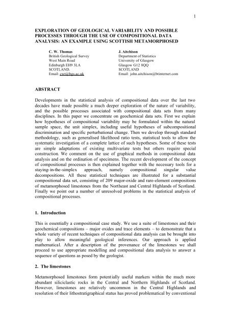
1EXPLORATION OF GEOLOGICAL VARIABILITY AND POSSIBLEPROCESSES THROUGH THE USE OF COMPOSITIONAL DATAANALYSIS: AN EXAMPLE USING SCOTTISH METAMORPHOSEDC. W. Thomas J. AitchisonBritish Geological SurveyDepartment of StatisticsWest Main RoadUniversity of GlasgowEdinburgh EH9 3LAGlasgow G12 8QQSCOTLAND.SCOTLANDEmail: cwt@bgs.ac.ukEmail: john.aitchison@btinternet.comABSTRACTDevelopments in the statistical analysis of compositional data over the last twodecades have made possible a much deeper exploration of the nature of variability,and the possible processes associated with compositional data sets from manydisciplines. In this paper we concentrate on geochemical data sets. First we explainhow hypotheses of compositional variability may be formulated within the naturalsample space, the unit simplex, including useful hypotheses of subcompositionaldiscrimination and specific perturbational change. Then we develop through standardmethodology, such as generalised likelihood ratio tests, statistical tools to allow thesystematic investigation of a complete lattice of such hypotheses. Some of these testsare simple adaptations of existing multivariate tests but others require specialconstruction. We comment on the use of graphical methods in compositional dataanalysis and on the ordination of specimens. The recent development of the conceptof compositional processes is then explained together with the necessary tools for astaying-in-the-simplex approach, namely compositional singular valuedecompositions. All these statistical techniques are illustrated for a substantialcompositional data set, consisting of 209 major-oxide and rare-element compositionsof metamorphosed limestones from the Northeast and Central Highlands of Scotland.Finally we point out a number of unresolved problems in the statistical analysis ofcompositional processes.1. IntroductionThis is essentially a compositional case study. We use a suite of limestones and theirgeochemical compositions – major oxides and trace elements – to demonstrate that awhole variety of recent techniques of compositional data analysis can be brought intoplay to allow meaningful geological inferences. Our approach is appliedmathematical. After a description of the provenance of the limestones we shallproceed to use appropriate modelling and compositional data analysis to answer asequence of questions as posed by the geologist.2. The limestonesMetamorphosed limestones form potentially useful markers within the much moreabundant siliciclastic rocks in the Central and Northern Highlands of Scotland.However, limestones are relatively uncommon in the Central Highlands andresolution of their lithostratigraphical status has proved problematical by conventional

2geological mapping. Limestones are more abundant in the Northern Highlands. Herethe discriminatory power of their geochemistry, established in areas of good exposureand well constrained lithostratigraphy, can prove useful in aiding lithographicalcorrelation areas of much poorer exposure.In this study we confine attention to two limestone data sets consisting 49 Dufftoenlimestones and 160 Inchrory limestones, each with 17-part geochemical compositions(Si, Al, Ti, Fe, Mg, Ca, Na, K, Mn, P, Loi,, Ba', Rb. Sr; V Y; Zr). The mainproblems considered in this study are to see how these may be considered as markerdata sets, investigating in full the nature of their differences. Also, since Inchrorylimestones are ‘younger’ than Dufftown limestones we consider how we may describethe process of change from one to the other.For more geological details see Thomas and Aitchison (1998)3. Are Duffinch and Inchrory limestones compositionally different?It is tempting to investigate this question by considering the lattice of Aitchison(1986, Section 7.5 and Fig. 7.3) whereby we would test whether the Duffinch andInchrory limestone compositions came from the same additive logistic normaldistributions. The fact that the distributional form of the compositional variabilitycannot be assumed to be logistic normal and that although we may attempt to fitmultivariate logistic skew normal distributions we would have to await a set ofcomprehensive multivariate skew normal tests before we could complete that route.But a simple examination of the estimated centres of the distributions of the majoroxides for Duffinch and Inchrory respectively::0.0496 0.0061 0.0003 0.0029 0.0136 0.5023 0.0007 0.0013 0.0002 0.0002 0.42290.1276 0.0270 0.0011 0.0106 0.0069 0.4540 0.0025 0.0050 0.0003 0.0007 0.3644will easily convince us that there are compositional differences between the twocompositional suites. Subsequent analysis, not dependent on distributional form willconfirm that there are substantial compositional differences between the twolimestones.4. What is the simplest way of discriminating between Duffinch and Inchrorylimestonesr?Aitchison (1986, Chapter 12) gave a number of practical situations wherecompositions play an explanatory or regressor role, where we may wish to see how acomposition is changed by different treatments, where in experiments with mixtureswe may attempt to determine the mixture which will provide the optimum response,and in classification or diagnostic problems where we may wish to use a compositionas a convenient or efficient means of determining type or to find out if anysubcomposition accounts for the substantive difference between the types.

3Binary logistic discrimination. For two types, such as the Duffinch and Inchrorylimestones here we may use binary logistic regression with logconstrasts of thecompositional components as the regressor; for a D-part composition x a logcontrastis defined aslc( α, x) = α log x1 + .. . + αDlog xD( α1 + .. . + αD= 0 ) .For two types (t = 0, t = 1) the binary logistic model is thus defined byexp{ α0+ lc( α , x)}pr( t = 0 | x) = 1 − pr( t = 1 | x)=1 + exp{ α + lc( α , x)}0.Maximum likelihood estimation of the parameter α is straightforward. The beauty ofthis model is that the adequacy of a subcomposition say (1, . . . , C) can readily betested since this hypothesis can be expressed as αC+ 1= . . . = αD= 0 . Thus the wholelattice of subcompositional hypotheses can be investigated and any adequatesubcomposition identified. Examples of this procedure can be found for hongitekongitediscrimination and Permian and post-Permian: discrimination in Aitchison(1986, Sections 12.6, 12.7).Figure 1 shows a portion of the substantial lattice of subcompositional hypotheseswith some of the more interesting subcompositions highlighted. The maximum modelat the top of the lattice retains the full 17-part composition as the explanatory variable.At the foot of the lattice is the hypothesis that compositional information is useless.At the next bottom level we have all the two-part subcompositions; at the next levelall the three-part subcompositions, and so on. In such lattice testing we usegeneralised likelihood ratio tests always testing the hypothesis within the maximummodel, starting with the simplest hypothesis, moving up the lattice to the next levelonly if we can reject all the hypotheses at the lower level and so on until we reach ahypothesis that we cannot reject. In the event that there are several non-rejectablehypotheses at a particular level that we either ‘accept’ the one with the smallestlikelihood ratio or move to the next level and ‘accept’ the hypothesis with the smallestlikelihood ratio. It should be remembered that in the absence of any loss structure in amultiple hypothesis situation all testing procedures are essentially ad hoc. We canonly report that we have found that this form of lattice testing usually leads to sensibleinferences.The dramatic result for limestones was reported in Thomas and Aitchison (1998),where out of the 17-part geochemical composition a 3-part subcomposition, namely(Fe, Mg, Ca), is found to be an adequate discriminator. The separation of the duffinchand inchrory limestones on the basis of the (Fe, Mg, Ca) subcomposition wasillustrated in a logratio scattergram, namely a (log(Fe/Ca), log(Mg/Ca)) plot. Weshow in Figure 2a the ternary diagram of the (Fe, Mg, Ca) subcompositions. Becauseof the smallness of Fe and Mg relative to Ca the subcompositional points crowd intothe Ca corner of the ternary diagram providing little illumination of the differences inthe duffinch and inchrory subcompositions. We can, however, use the device of acentering perturbation *von Eynatten, Pawlowsky-Glahn and Mateu Figueras, 2002)to provide a clearer picture of the separation. This is shown in Figure 2b, together

4with the perturbed dividing logcontrast line which separates Duffinch fromInchrory..We record that the estimated logcontrast discriminator is6.98 +4.84 log Fe – 3.05 log Mg – 1.79 log Ca.It is worth commenting here that prior to this analysis, reliance on spider diagramshad suggested strongly that discrimation between the two limestones lay in thesiliciclastic component, the (Si, Ti, Al, K, Rb, V) subcomposition, not in thecarbonate component, the subcomposition (Fe, Mg, Ca). In the lattice of Figure 1 weshow the results for the siliciclastic subcomposition. It is quite clear that thehypothesis that this had a differentiating effect has to be strongly rejected.Another worthwhile comment here is about the use of perturbation, the operation ofchange in compositions. The use above in the ternary diagram is an excellent devicefor the provision of simpler visual interpretation of ternary scattergrams. The readerwill have noticed that we have used the 11 major oxides (proportion by weight) and 6trace elements (parts per million) as if these constituted a single composition, despitethe fact that they are measured in different units. The reason for this is that it requiresonly a simple constant perturbation to attain common units. And such perturbationshave useful invariance properties. In the present context it is simple to demonstratethat such a perturbation would affect only the value of α 0in the binary logistic modeland this has no relevance within the lattice testing procedure. See Aitchison (2003) forfurther comment.5. What is the nature of the change between duffinch and inchrory limestones?Inchrory limestones are younger than Dufftown limestones and so it is reasonable toask whether we can describe how a generic Inchrory limestone may be altered into ageneric Dufftown limestone. We confine our discussion to the major oxidecompositions. We recall that the operation of change for compositions is aperturbation Suppose that x and X denotes the compositions of generic Inchrory andDufftown limestones and that X arises as a perturbation p of x, namely, X = p ⊕ x .Then we know that in terms of centres of the distributionsso thatcen( X ) = cen( p) ⊕ cen( x),cen( p) = cen( X ) Θ cen( x),and is easily determined from the centres in Section 3 asSi Al Ti Fe Mg Ca Na K Mn P Loi0.0554 0.0321 0.0381 0.0394 0.2823 0.1578 0.0390 0.0366 0.1038 0.0499 0.1655We have in our modelling allowed the perturbations to be variable and are using thecentre of these to give an indication of the nature of the perturbation, This centre is, of

5course, exactly what we obtain if we assumed that there was a constant perturbation atwork.First we note a trivial point, namely that the there is near equality pf the Ca and Loicomponents. This is simply recording the stability of the (Ca, Loi) subcomposition, inother words the fact that Loi will always match the Ca component.Second, since we saw the importance of the (Fe, Mg, Ca) subcomposition indiscriminating between the two liimestones we note the considerable differences inthe perturbation components of these oxides, namely [0.0394 0.2823 0.1578],showing how in the change from Inchrory to Dufftown Fe has given way substantiallyto Mg and less so to Ca. The perturbation components of all the other oxides rxceptfrom Mn are reasonable constant indicating stability of the associatedsubcomposition. The question then arises: is there some geological explanation fo therelative increase in Mn?6. Are there any helpful graphical representations of the variability in thelimestones?We have already seen the use of a logratio scattergram to demonstrate the separationbetween Duffinch and Inchrory limestones. There is hopefully no need to repeat thewarnings of Chayes and others on the misuse of such other graphical tools such asHarker diagrams. We have also seen the use of a centering perturbation to improvethe use of a ternary diagram to show the relevance of the carbonate (Fe, Mg, Ca)subcomposition as a discriminator between the Duffinch and Inchrory.limestones.The main advance in other graphical descriptions of compositional variability hasbeen the extension of the familiar and powerful unconstrained biplot technique tocompositional data; see Aitchison (1990b, 1997, 2001) and Aitchison and Greenacre(2002) for details. We are currently exploring these and will present an example atCODAWORK03.7. Is it possible to order specimens within the limestone suites?If it is assumed that there is a process of change from Inchrory-ness to Dufftown-nesscan we somehow order the limestones within this process there are simplecompositional more or less equivalent ways of doing this. From the discriminationanalysis we can compute for each limestone the probability of allocation to theInchrory set and arrange these probabilities in decreasing order. Or we use theprincipal logcontrast component (Aitchison, 1986, Section 8.3) or equivalently by useof the first coefficients in a singular value decomposition (Aitchison, 2003). Withsuch techniques it is also possible to interpret the possible position of other non-Inchrory, non Duffinch limestones with the Inchrory to Duffinch process. We do notreport details here; for some earlier results, see Thomas and Aitchison (1998).

68. Can we identify possible compositional processes from the limestone data?Aitchison and Thomas (1998) explained how modern compositional data analysiscould be used to investigate identify and analyse possible compositional processes,using two simple examples: Arctic lake sediments to identify the process in relation todepth and simple olivine data to identify possible equilibrium relationships. Thestatistical technique used depended largely on compositional regression analysis andlogcontrast principal component analysis. In a complementary paper Aitchison andBarceló-Vidal (2002) used compositional singular value decompositions to provide astaying-in-the-simplex approach where the compositions of the data set are expressedas power-perturbation combinations. Thus for an N × D compositional data matrixwith nth row the composition x nthe singular value composition provides theexpressionx = ξ$ ⊕ ( u1p1 ⊗ b1 ) ⊕ . .. ⊕ ( u p ⊗ b ) ,n n nR R Rwhere ξ $ is the estimate of the centre of the data set, and pi ( i = 1 , . . . , R)are positive‘singular values’ in descending order of magnitude, the bi ( i = 1 , . . . , R)areorthogonal compositions, R is a readily defined rank of the compositional data set andthe u’s are power components specific to each composition. . In practice R iscommonly D − 1, the full dimension of the simplex. In a way similar to that for dataDsets in R we may consider an approximation of order r < R to the compositionaldata set given bySuch an approximation retains a proportionx ( r ) = $ ⊕ ( u p ⊗ b ) ⊕ . .. ⊕ ( u p ⊗ b ).nξn1 1 1nr r r2 2 2 2( p + .. . + p ) / ( p + . .. + p )1rof the total variability of the N × D compositional data matrix as measured by thetrace of the estimated centered logratio covariance matrix or equivalently in terms ofthe total mutual squared distances as−1 2{ N ( N − 1)} ∆ ( x , x ).D∑m

70.0675 0.0622 0.0788 0.0724 0.1254 0.1102 0.0560 0.0701 0.1460 0.0991 0.11230.0993 0.1111 0.1080 0.1028 0.0709 0.0807 0.0389 0.1190 0.0815 0.1076 0.08030.0674 0.0810 0.0899 0.0765 0.0422 0.1190 0.1011 0.0845 0.0899 0.1354 0.1132with successive degrees of approximation 0.46, 0.69, 0.84, 0.92.We note that in the first approximation the major relative increase is in Ca and to alesser extent Si. At the second approximation, both Mg and Ca show a relativeincrease and the increase in Mn seen earlier is also evident. At the thirdapproximation the main feature seems to be some relative depletion of Na, to arelative gain in K? And so on in a tentative interpretation.There are substantial statistical deficiencies in this area of compositional dataanalysis. For example at the various stages of approximation the near equality of asubset of components suggests that the corresponding subcomposition is stable forthat stage. But can we devise suitable statistical tests of such a subcompositionalstability hypothesis, Also although the singular value decomposition is identifyingorthogonal aspects of the process it may be that some other representation, say of thefirst two stages may provide a more enlightening view of the process. This would be arestructuring rather similar to the varimax technique in principal component analysis,but how should it be done compositionally? Again, suppose that the geologist suggestthat there may be two basic processes at work, possibly independently, a carbonateand a siliciclastic process. A possible method of modelling might then be to setx = $ ( u π ⊗ β ) ⊕ ( u π ⊗ β ) ⊕ p,n n1 1 1 n2 2 2where β1, β2are D-part compositions somehow representing carbonate andsiliciclastic subcompositions, but how, π1, π2are parameters representing the extentof the carbonate and siliciclastic importance and requiring estimation, the ucoordinates again requiring to be determined and the p a composition, rather like theerror term in a regression analysis. It is obvious that there is much statistical researchremaining to be done in this important area of compositional data analysis. We arecurrently working in this area and will certainly report any new work atCODAWORK03.REFERENCESAitchison, J., 1986, The Statistical Analysis of Compositional Data: Chapman andHall, London. Reprinted in 2003 with additional material by The Blackburn Press.Aitchison, J., 1990, Relative variation diagrams for describing patterns of variabilityof compositional data: Math. Geology, v. 22, p. 487-512.Aitchison, J., 1997, The one-hour course in compositional data analysis orcompositional data analysis is easy, in Pawlowsky Glahn, V., ed., Proceedings of theThird Annual Conference of the International Association for Mathematical Geology:CIMNE, Barcelona, p. 3-35.

8Aitchison, J., 2001, Simplicial inference, in Viana, M.A.G. and Richards, D.St.P.,eds., Algebraic Methods in Statistics and Probability: Contemporary MathematicsSeries 287, American Mathematical Society, Providence, Rhode Island, p. 1-22.Aitchison, J., 2003. Compositional data analysis: where are we and where are weheading? : paper at CODAWORK03.Aitchison, J. and Barceló-Vidal, C., 2002,. Compositional processes: a statisticalsearch for understanding, in Proceedings of the Eighth Annual Conference of theInternational Association for Mathematical Geology, to appear.Aitchison, J. and Greenacre, M., 2002, Biplots for compositional data: Appl. Statist.,v. 51.. p. 375-382.Aitchison, J. and Thomas, C. W. (1998) Differential perturbation processes: a tool forthe study of compositional processes. In Proceedings of the Fourth AnnualConference of the International Association for Mathematical Geology (Buccianti A.,Nardi, G. and Potenza, R., eds), pp. 499-504. Naplesi: De Frede.Thomas, C. W. and Aitchison, J. (1998). The use of logratios in subcompositionalanalysis and geochemical discrimination of metamorphosed limestones from thenortheast and central Scottish Highlands. In: A. Buccianti, G. Nardi and R. Potenza,Eds., Proceedings of IAMG98, The Fourth Annual Conference of the InternationalAssociation for Mathematical Geology, De Frede, Naples, 549-554...von Eynatten, H,. Pawlowsky-Glahn and MateuFigueras, G., 2002, Understandingperturbation on the simplex: a simple method to better visualise and interpretcompositional data in ternary diagrams: Math. Geology, v. 34, p. 249-257.