Transient Analysis of a Cantilever Beam - University of Alberta

http://www.mece.ualberta.ca/tutorials/ansys/CL/CIT/Transient/Print.html
Transient Analysis of a Cantilever Beam
Introduction
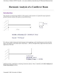
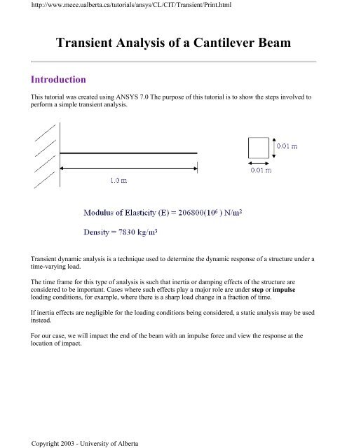
This tutorial was created using ANSYS 7.0 The purpose of this tutorial is to show the steps involved to
perform a simple transient analysis.
Transient dynamic analysis is a technique used to determine the dynamic response of a structure under a
time-varying load.
The time frame for this type of analysis is such that inertia or damping effects of the structure are
considered to be important. Cases where such effects play a major role are under step or impulse
loading conditions, for example, where there is a sharp load change in a fraction of time.
If inertia effects are negligible for the loading conditions being considered, a static analysis may be used
instead.
For our case, we will impact the end of the beam with an impulse force and view the response at the
location of impact.
Copyright 2003 - University of Alberta

http://www.mece.ualberta.ca/tutorials/ansys/CL/CIT/Transient/Print.html
Since an ideal impulse force excites all modes of a structure, the response of the beam should contain all
mode frequencies. However, we cannot produce an ideal impulse force numerically. We have to apply a
load over a discrete amount of time dt.
After the application of the load, we track the response of the beam at discrete time points for as long as
we like (depending on what it is that we are looking for in the response).
The size of the time step is governed by the maximum mode frequency of the structure we wish to
capture. The smaller the time step, the higher the mode frequency we will capture. The rule of thumb in
ANSYS is
time_step = 1 / 20f
where f is the highest mode frequency we wish to capture. In other words, we must resolve our step size
such that we will have 20 discrete points per period of the highest mode frequency.
It should be noted that a transient analysis is more involved than a static or harmonic analysis. It
requires a good understanding of the dynamic behavior of a structure. Therefore, a modal
analysis of the structure should be initially performed to provide information about the
structure's dynamic behavior.
In ANSYS, transient dynamic analysis can be carried out using 3 methods.
Copyright 2003 - University of Alberta

http://www.mece.ualberta.ca/tutorials/ansys/CL/CIT/Transient/Print.html
The Full Method: This is the easiest method to use. All types of non-linearities are allowed. It is
however very CPU intensive to go this route as full system matrices are used.
The Reduced Method: This method reduces the system matrices to only consider the Master
Degrees of Freedom (MDOFs). Because of the reduced size of the matrices, the calculations are
much quicker. However, this method handles only linear problems (such as our cantilever case).
The Mode Superposition Method: This method requires a preliminary modal analysis, as
factored mode shapes are summed to calculate the structure's response. It is the quickest of the
three methods, but it requires a good deal of understanding of the problem at hand.
We will use the Reduced Method for conducting our transient analysis. Usually one need not go further
than Reviewing the Reduced Results. However, if stresses and forces are of interest than, we would have
to Expand the Reduced Solution.
ANSYS Command Listing
finish
/clear
/TITLE, Dynamic Analysis
/FILNAME,Dynamic,0 ! This sets the jobname to 'Dynamic'
/PREP7 ! Enter preprocessor
K,1,0,0 ! Keypoints
K,2,1,0
L,1,2 ! Connect keypoints with line
ET,1,BEAM3 ! Element type
R,1,0.0001,8.33e-10,0.01 ! Real constants
MP,EX,1,2.068e11 ! Young's modulus
MP,PRXY,1,0.33 ! Poisson's ratio
MP,DENS,1,7830 ! Density
LESIZE,ALL,,,10 ! Element size
LMESH,1 ! Mesh the line
FINISH
/SOLU ! Enter solution phase
ANTYPE, TRANS ! Transient analysis
TRNOPT,REDUC, ! reduced solution method
DELTIM,0.001 ! Specifies the time step sizes
!At time equals 0s
NSEL,S,,,2,11, ! select nodes 2 - 11
M,All,UY, , , ! Define Master DOFs
NSEL,ALL ! Reselect all nodes
D,1,ALL ! Constrain left end
F,2,FY,-100 ! Load right end
!*
Copyright 2003 - University of Alberta

http://www.mece.ualberta.ca/tutorials/ansys/CL/CIT/Transient/Print.html
!At time equals 0.001s
TIME,0.001 ! Sets time to 0.001 seconds
KBC,0 ! Ramped load step
FDELE,2,ALL ! Delete the load at the end
!*
!At time equals 1s
TIME,1 ! Sets time to 1 second
KBC,0 ! Ramped load step
!*
LSSOLVE,1,3,1 ! solve multiple load steps
FINISH
/POST26 ! Enter time history
FILE,'Dynamic','rdsp','.' ! Calls the dynamic file
NSOL,2,2,U,Y, UY_2 ! Calls data for UY deflection at node 2
STORE,MERGE ! Stores the data
PLVAR,2, ! Plots vs. time
!Please note, if you are using a later version of ANSYS,
!you will probably have to issue the LSWRITE command at the
!end of each load step for the LSSOLVE command to function
!properly. In this case, replace the !* found in the code
!with LSWRITE and the problem should be solved.
Copyright 2003 - University of Alberta