PDF (5143 kByte) - WIAS
PDF (5143 kByte) - WIAS
PDF (5143 kByte) - WIAS

You also want an ePaper? Increase the reach of your titles
YUMPU automatically turns print PDFs into web optimized ePapers that Google loves.
4<br />
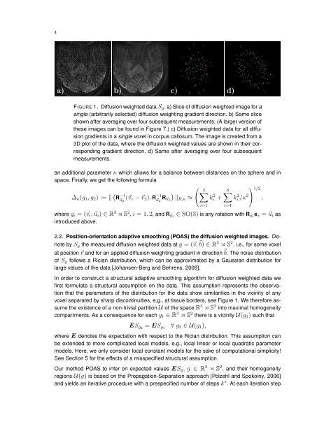
a) b) c) d)<br />
FIGURE 1. Diffusion weighted data Sg. a) Slice of diffusion weighted image for a<br />
single (arbitrarily selected) diffusion weighting gradient direction. b) Same slice<br />
shown after averaging over four subsequent measurements. (A larger version of<br />
these images can be found in Figure 7.) c) Diffusion weighted data for all diffusion<br />
gradients in a single voxel in corpus callosum. The image is created from a<br />
3D plot of the data, where the diffusion weighted values are shown in their corresponding<br />
gradient direction. d) Same after averaging over four subsequent<br />
measurements.<br />
an additional parameter κ which allows for a balance between distances on the sphere and in<br />
space. Finally, we get the following formula<br />
<br />
3<br />
k 2 6<br />
i + k 2 i /κ 2<br />
1/2 ,<br />
∆κ(g1, g2) := R −1<br />
u2 (v1 − v2), R −1<br />
u2 Ru1<br />
<br />
R,κ ≈<br />
where gi = (vi, ui) ∈ R 3 ⋊ S 2 , i = 1, 2, and Rui ∈ SO(3) is any rotation with Rui ez = ui as<br />
introduced above.<br />
2.2. Position-orientation adaptive smoothing (POAS) the diffusion weighted images. De-<br />
note by Sg the measured diffusion weighted data at g = (v, b) ∈ R 3 ⋊ S 2 , i.e., for some voxel<br />
at position v and for an applied diffusion weighting gradient in direction b. The noise distribution<br />
of Sg follows a Rician distribution, which can be approximated by a Gaussian distribution for<br />
large values of the data [Johansen-Berg and Behrens, 2009].<br />
In order to construct a structural adaptive smoothing algorithm for diffusion weighted data we<br />
first formulate a structural assumption on the data. This assumption represents the observation<br />
that the parameters of the distribution for the data show similarities in the vicinity of any<br />
voxel separated by sharp discontinuities, e.g., at tissue borders, see Figure 1. We therefore assume<br />
the existence of a non-trivial partition U of the space R 3 ⋊ S 2 into maximal homogeneity<br />
compartments. As a consequence for each g1 ∈ R 3 ⋊ S 2 there is a vicinity U(g1) such that<br />
i=1<br />
ESg2 = ESg1 ∀ g2 ∈ U(g1),<br />
where E denotes the expectation with respect to the Rician distribution. This assumption can<br />
be extended to more complicated local models, e.g., local linear or local quadratic parameter<br />
models. Here, we only consider local constant models for the sake of computational simplicity!<br />
See Section 5 for the effects of a misspecified structural assumption.<br />
Our method POAS to infer on expected values ESg, g ∈ R 3 ⋊ S 2 , and their homogeneity<br />
regions U(g) is based on the Propagation-Separation approach [Polzehl and Spokoiny, 2006]<br />
and yields an iterative procedure with a prespecified number of steps k ∗ . At each iteration step<br />
i=4