PDF (5143 kByte) - WIAS

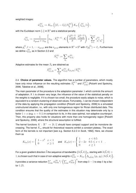
weighted images:
˜w (k)
:= Kloc ||v1 − v2||/h v1v2 (k)
Kst z
bl
(k)
v1v2 /λ
,
with the Euclidean norm . in R3 and a statistical penalty
z (k)
v1v2 :=
1
ˆS (k−1)
(k−1) (v1,0)
nS0 · Ñ · K
v1
ngrad + nS0
ˆσ ,
ˆS (k−1) ngrad
(v2,0)
+
ˆσ
l=1
s (k)
g (l)
1 g(l)
2
where g (l)
1 , l = 1, · · · ngrad, are the ngrad elements in R 3 ⋊ S 2 with v(g (l)
1 ) = v1. Furthermore
we define s (k)
g1g2 as in Section 2.2 and
Ñ (k)
v1 :=
Adaptive estimates for the mean ¯ S0 are obtained as
ˆS (k)
(v1,0) =
v2
v2
˜w (k)
v1v2 .
˜w (k) ¯S(v2,0)/
(k)
Ñ v1v2
v1 .
2.4. Choice of parameter values. The algorithm has a number of parameters, which mostly
have only minor influence on the resulting estimates ˆ S (k∗ )
g
2006, Tabelow et al., 2008].
7
and ˆ S (k∗ )
(v,0) [Polzehl and Spokoiny,
The main parameter of the procedure is the adaptation parameter λ which controls the amount
of adaptation. If λ is chosen very large, the influence of the value of the statistical penalty on
the weights is negligible. If it is chosen too small, the procedure easily adapts to noise, which is
equivalent to a random clustering of observed values. Fortunately, λ can be chosen independent
of the data by applying the propagation condition [Polzehl and Spokoiny, 2006] to a simulated
unstructured situation, i.e., with only one homogeneous region for Rician distributed data. This
condition ensures that the quality of the estimates in this situation may deteriorate only by a
factor 1 + α (e.g. α = 0.1) in comparison to its, in this case optimal, non-adaptive counterpart.
Then, this property also holds for situations with more than one homogeneity region [Polzehl
and Spokoiny, 2006], where the structural assumption is fulfilled.
The kernel functions K : R + → [0, 1] should have compact support and be monotone decreasing.
The kernel Kst should for theoretical reasons exhibit a constant plateau. The exact
form of the kernels is not important [see e.g. Section 6.2.3 in Scott, 1992]. Here, we choose
them as
Kloc(x) =
1 − x 2 x < 1
0 x ≥ 1
⎧
⎨ 1 x < 0.5
and Kst(x) = 2 − 2x
⎩
0
0.5 ≤ x < 1
x ≥ 1
For a given gradient directionb the sequence of bandwidths {h( b, k)}k, starting with h( b, 0) =
1, is chosen such that in case of non-adaptive weights ¯w (k)
g1g2 = Kloc ∆κ( b,k) (g1, g2) /h(
b, k) ,
it provides a variance reduction 2 2 /
from step k − 1 to step k by a fac-
tor 1.25.
g2 ¯w(k)
g1g2
g2 ¯w(k)
g1g2
.