Economic Equilibrium Modeling with GAMS

4
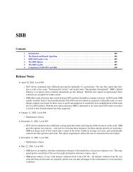
Figure 1. An Indi erence Curve
Y
4
1
1 3
on the preferences of a single consumer, the indi erence curve is a line which connects
all combinations of two goods x and y between which our consumer is indi erent. As
this curve is drawn, we have represented an agent with well-behaved preferences: at
any allocation, more is better (monotonicity), and averages are preferred to extremes
(convexity). Exactly one indi erence curve goes through each positive combination of x
and y. Higher indi erence curves lie to the north-east.
If we wish to characterize an agent's preferences, the marginal rate of substitution
(MRS) is a useful point of reference. At a given combination of x and y, the marginal
rate of substitution is the slope of the associated indi erence curve. As drawn, the MRS
increases in magnitude as we move to the northwest and the MRS decreases as we move
to the south east. The intuitive understanding is that the MRS measures the willingness
of the consumer to trade o one good for the other. As the consumer has greater amounts
of x, she will be willing to trade more units of x for each additional unit of y { this results
from convexity.
An ordinal utility function U(x; y) provides a helpful tool for representing preferences.
This is a function which associates a number with each indi erence curve. These numbers
increase as we move to the northeast, with each successive indi erence curve representing
bundles which are preferred over the last. The particular number assigned to an indi erence
curve has no intrinsic meaning. All we know is that if U(x1;y1) > U(x2;y2), then the
consumer prefers bundle 1 to bundle 2.
Figure 2 illustrates how it is possible to use a utility function to generate a diagram
with the associated indi erence curves. This gure illustrates Cobb-Douglas well-behaved
preferences which are commonly employed in applied work.
Up to this point, we have wehave focused exclusively on the characterization of preferences.
Let us now consider the other side of the consumer model { the budget constraint.
The simplest approach tocharacterizing consumer income is to assume that the consumer
has a xed money income which she may spend on any goods. The only constraint on this
choice is that the value of the expenditure may not exceed the money income. This is the
standard budget constraint:
Pxx + Pyy = M:
X