GDXMRW: Interfacing GAMS and MATLAB
GDXMRW: Interfacing GAMS and MATLAB
GDXMRW: Interfacing GAMS and MATLAB

Create successful ePaper yourself
Turn your PDF publications into a flip-book with our unique Google optimized e-Paper software.
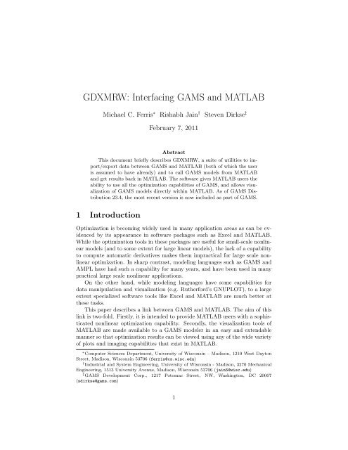
<strong>GDXMRW</strong>: <strong>Interfacing</strong> <strong>GAMS</strong> <strong>and</strong> <strong>MATLAB</strong><br />
Michael C. Ferris ∗ Rishabh Jain † Steven Dirkse ‡<br />
February 7, 2011<br />
Abstract<br />
This document briefly describes <strong>GDXMRW</strong>, a suite of utilities to import/export<br />
data between <strong>GAMS</strong> <strong>and</strong> <strong>MATLAB</strong> (both of which the user<br />
is assumed to have already) <strong>and</strong> to call <strong>GAMS</strong> models from <strong>MATLAB</strong><br />
<strong>and</strong> get results back in <strong>MATLAB</strong>. The software gives <strong>MATLAB</strong> users the<br />
ability to use all the optimization capabilities of <strong>GAMS</strong>, <strong>and</strong> allows visualization<br />
of <strong>GAMS</strong> models directly within <strong>MATLAB</strong>. As of <strong>GAMS</strong> Distribution<br />
23.4, the most recent version is now included as part of <strong>GAMS</strong>.<br />
1 Introduction<br />
Optimization is becoming widely used in many application areas as can be evidenced<br />
by its appearance in software packages such as Excel <strong>and</strong> <strong>MATLAB</strong>.<br />
While the optimization tools in these packages are useful for small-scale nonlinear<br />
models (<strong>and</strong> to some extent for large linear models), the lack of a capability<br />
to compute automatic derivatives makes them impractical for large scale nonlinear<br />
optimization. In sharp contrast, modeling languages such as <strong>GAMS</strong> <strong>and</strong><br />
AMPL have had such a capability for many years, <strong>and</strong> have been used in many<br />
practical large scale nonlinear applications.<br />
On the other h<strong>and</strong>, while modeling languages have some capabilities for<br />
data manipulation <strong>and</strong> visualization (e.g. Rutherford’s GNUPLOT), to a large<br />
extent specialized software tools like Excel <strong>and</strong> <strong>MATLAB</strong> are much better at<br />
these tasks.<br />
This paper describes a link between <strong>GAMS</strong> <strong>and</strong> <strong>MATLAB</strong>. The aim of this<br />
link is two-fold. Firstly, it is intended to provide <strong>MATLAB</strong> users with a sophisticated<br />
nonlinear optimization capability. Secondly, the visualization tools of<br />
<strong>MATLAB</strong> are made available to a <strong>GAMS</strong> modeler in an easy <strong>and</strong> extendable<br />
manner so that optimization results can be viewed using any of the wide variety<br />
of plots <strong>and</strong> imaging capabilities that exist in <strong>MATLAB</strong>.<br />
∗ Computer Sciences Department, University of Wisconsin – Madison, 1210 West Dayton<br />
Street, Madison, Wisconsin 53706 (ferris@cs.wisc.edu)<br />
† Industrial <strong>and</strong> System Engineering, University of Wisconsin - Madison, 3270 Mechanical<br />
Engineering, 1513 University Avenue, Madison, Wisconsin 53706 (jain5@wisc.edu)<br />
‡ <strong>GAMS</strong> Development Corp., 1217 Potomac Street, NW, Washington, DC 20007<br />
(sdirkse@gams.com)<br />
1
2 Installation<br />
This section describes the installation procedure for all machines. The following<br />
section describes the testing procedure for verifying a correct installation.<br />
First of all, you need to install both <strong>MATLAB</strong> <strong>and</strong> <strong>GAMS</strong> on your machine.<br />
For brevity, we will assume that the <strong>GAMS</strong> system (installation) directory is<br />
(for Windows)<br />
c:\gams<br />
<strong>and</strong> for non-Windows systems:<br />
/usr/local/gams<br />
All of the utilities come as a part of the <strong>GAMS</strong> distribution, so to use them<br />
you have only to add the <strong>GAMS</strong> directory to the <strong>MATLAB</strong> path. One way to<br />
do this is from the <strong>MATLAB</strong> comm<strong>and</strong> prompt, as follows:<br />
>> addpath ’C:\gams’; savepath;<br />
OR this can be done by following these steps:<br />
1. Start <strong>MATLAB</strong><br />
2. Click on ’File’ tab.<br />
3. Now click on ’Set Path’<br />
4. Click on ’Add Folder’<br />
5. Select <strong>GAMS</strong> directory <strong>and</strong> click ’OK’.<br />
6. Save it <strong>and</strong> then close it.<br />
3 Testing<br />
The <strong>GAMS</strong> system comes with some tests that you should run to verify the<br />
correct configuration <strong>and</strong> operation of the <strong>GDXMRW</strong> utilities. In addition,<br />
these tests create a log file that can be useful when things don’t work as expected.<br />
To run the tests, carry out the following steps.<br />
1. Create a directory to run the tests in, e.g.<br />
% mkdir \tmp<br />
2. Extract the test models <strong>and</strong> supporting files from the <strong>GAMS</strong> test library<br />
into the test directory.<br />
% cd \tmp<br />
% testlib gdxmrw03<br />
% testlib gdxmrw04<br />
% testlib gdxmrw05<br />
2
3. Execute the <strong>GAMS</strong> files gdxmrw03 <strong>and</strong> gdxmrw04. These files test that<br />
’rgdx’ <strong>and</strong> ’wgdx’ are working properly. In addition to calling <strong>MATLAB</strong><br />
in batch mode, they verify that the data are read <strong>and</strong> written as expected<br />
<strong>and</strong> give a clear indication of success or failure.<br />
4. The <strong>GAMS</strong> file gdxmrw05 tests the ’gams’ utility. Like the other tests,<br />
it can be run in batch mode. You can also run it interactively by starting<br />
<strong>MATLAB</strong>, making tmp the current directory, <strong>and</strong> running the script<br />
“testinst.m”.<br />
>> testinst<br />
In addition to messages indicating success or failure, this test produces a<br />
log file testinstlog.txt that will be useful in troubleshooting a failed<br />
test.<br />
4 Data Transfer<br />
This paper suggests a better approach to import <strong>and</strong> export data from <strong>GAMS</strong><br />
to <strong>MATLAB</strong> using GDX files. GDX is <strong>GAMS</strong> Data Exchange file. This is a<br />
platform independent file that stores data efficiently in binary format. Unlike<br />
flat files, which might be machine dependent, GDX file are machine independent.<br />
Data in GDX file is stored in sparse format <strong>and</strong> is consistent with no<br />
duplication, contradiction or syntax errors, making it a better tool to store data<br />
than flat files. In this paper we are going to explain three <strong>MATLAB</strong> routines,<br />
namely ’rgdx’, ’wgdx’ <strong>and</strong> ’gams’. The first two are used to read <strong>and</strong> write data<br />
from a GDX file into <strong>MATLAB</strong> <strong>and</strong> the third routine will take user input to<br />
execute a gams model from <strong>MATLAB</strong> <strong>and</strong> get results back in <strong>MATLAB</strong>. All of<br />
these routines are such designed to get data in almost same form as is stored in<br />
a GDX file.<br />
One of the most important features of a GDX file that we are going use in<br />
this paper is its UEL, Unique Element List. GDX files have only one global<br />
UEL <strong>and</strong> every element is mapped to this UEL. Thus ’rgdx’ output will contain<br />
a global UEL as one of its fields. To write data into a GDX file, a user can enter<br />
a local UEL for each symbol <strong>and</strong> ’wgdx’ will create one global UEL; otherwise<br />
it will create a default UEL ranging from 1 to n.<br />
4.1 rgdx<br />
rgdx is the <strong>MATLAB</strong> utility to import data from a GDX file. It takes structural<br />
input <strong>and</strong> returns data back in the form of a structure. This is a very flexible<br />
routine as it gives user control over the output data structure. rgdx can read<br />
set/parameter/equation/variable from a GDX file <strong>and</strong> display results in either<br />
full/dense or sparse form. A user can also perform a filtered read to read only<br />
certain specific elements of a symbol. It can also perform compression to remove<br />
3
extra zeros.<br />
This routine can take up to two arguments. The first argument is a string<br />
input containing the GDX file name. It can be with or without the ’.gdx’ file<br />
extension. If you call this routine with only the GDX file name as an argument<br />
then the ’uels’ field of output structure will be the global UEL of the GDX file<br />
<strong>and</strong> the rest of the fields of the output structure will be NULL. The second argument<br />
is a structure input containing information regarding the desired symbol.<br />
The syntax for this call will look like:<br />
x = rgdx(’fileName’, structure);<br />
As an example, we read a 3D parameter, ’test3’ from ’sample.gdx’. Here we<br />
want to display this parameter in full format but without redundant zeros. e.g.<br />
>> s.name = ’test3’;<br />
>> s.form = ’full’;<br />
>> s.compress = true;<br />
>> x = rgdx(’sample’, s)<br />
x =<br />
name: ’test3’<br />
type: ’parameter’<br />
dim: 3<br />
val: [4x2x2 double]<br />
form: ’full’<br />
uels: {{1x4 cell} {1x2 cell} {1x2 cell}}<br />
>> x.val<br />
ans(:,:,1) =<br />
3 4<br />
4 5<br />
5 6<br />
6 7<br />
ans(:,:,2) =<br />
4 5<br />
5 6<br />
6 7<br />
7 8<br />
4
x.uels{1}<br />
ans =<br />
’1’ ’2’ ’3’ ’4’<br />
>> x.uels{2}<br />
ans =<br />
’j1’ ’j2’<br />
>> x.uels{3}<br />
ans =<br />
’k1’ ’k2’<br />
In the following subsections we will explain the input <strong>and</strong> output structures.<br />
Please note that except for the ’name’ <strong>and</strong> ’uels’ fields, all other string fields take<br />
case insensitive input. All boolean fields can also be entered as string values as<br />
well.<br />
4.1.1 Input structure<br />
To read a symbol from a GDX file we just need to know its name in string<br />
format. Thus, the only m<strong>and</strong>atory field of the input structure is ’name’. e.g.<br />
>> s.name = ’test3’;<br />
There are several other optional fields of the input structure that give user<br />
more control over the output sturcture. These optional fields are as follows:<br />
1. form<br />
This field represents the form of the output data. Output data can be<br />
either in ’full’ or ’dense’ form or it can be in [i, j,.., val] form. In this<br />
paper we will label [i, j,.., val] as ’sparse’. A user can enter it as string<br />
input with value ’full’ or ’sparse’. e.g.<br />
>> s.form = ’full’;<br />
By default the data will be in ’sparse’ format.<br />
2. compress<br />
By default the uels in the output structure will be a global UEL of the<br />
GDX file <strong>and</strong> the ’val’ field data will be indexed to this UEL. The rgdx<br />
routine allows a user to remove rows <strong>and</strong> columns with all zeros from<br />
the ’val’ data matrix <strong>and</strong> re-indexes the uels accordingly. This is called<br />
5
compression of the data. This can be achieved by setting compress as true<br />
in the input structure. Valid values for this field are true <strong>and</strong> false, either<br />
in logical form or in string form. e.g.<br />
>> s.compress = ’true’;<br />
3. uels<br />
This input field is used to perform a filtered read i.e. output data matrix<br />
will contain values only corresponding to the entered uels. Filtered read<br />
is very useful if user just wants certain specific set of data. Uels should be<br />
entered in cell array form. It has to be in 1xN form with each column being<br />
a cell array representing the uels for that dimension. Each column can<br />
have strings, doubles or combinations of both. It also allow user to enter<br />
double data in shorth<strong>and</strong> notation or a 1 x N matrix. For example, in the<br />
previous example we can perform a filtered read to get data corresponding<br />
to only the ’1’, ’3’ elements of the first index of the parameter ’test3’.<br />
>> s.uels = {{1 3}, {’j1’, ’j2’}, {’k1’, ’k2’}};<br />
>> s.compress = false;<br />
>> x = rgdx(’sample’, s)<br />
x =<br />
name: ’test3’<br />
type: ’parameter’<br />
dim: 3<br />
val: [2x2x2 double]<br />
form: ’full’<br />
uels: {{1x2 cell} {1x2 cell} {1x2 cell}}<br />
>> x.val<br />
ans(:,:,1) =<br />
3 4<br />
5 6<br />
ans(:,:,2) =<br />
4 5<br />
6 7<br />
Here it should be noted that we turned off compression while performing<br />
the filtered read. This is necessary because the filtered read will give data<br />
6
in accordance with the entered uels <strong>and</strong> the output uels will be the same<br />
as the input uels; thus compression is not possible.<br />
4. field<br />
This field is required when variables or equations are to be read from a<br />
GDX file. Sets <strong>and</strong> parameters in the GDX file do not have any field value<br />
but variables <strong>and</strong> equations have 5 fields namely, level, marginal, lower,<br />
upper <strong>and</strong> scale. Thus, it may be useful to enter field as an input when<br />
reading an equation or a variable. A user can enter it as a string with<br />
valid values being ’l/m/up/lo/s’. e.g.<br />
>> s.field = ’m’;<br />
By default, the output will be the level value of a variable or an equation.<br />
5. ts<br />
This represents the text string associated with the symbol in the GDX<br />
file. If a user sets this field as ’true’, then the output structure will have<br />
one more string field ’ts’ that contains the text string of the symbol. e.g.<br />
>> s.ts = true;<br />
6. te<br />
<strong>GAMS</strong> allows a modeler to enter text elements for a set. Similarly to<br />
the ’ts’ field, if a user sets ’te’ to be true in the input structure, then the<br />
output structure will contain one more field representing the text elements<br />
for that symbol. Please note that text elements only exist for ’sets’. e.g.<br />
>> s.te = true;<br />
4.1.2 Output Structure<br />
As mentioned earlier, output of the rgdx routine will be in structure form. This<br />
structure is very similar to the input structure. To get information regarding<br />
any symbol, we always need to display its basic characteristics, such as its name,<br />
type, value, uels, form, etc. An output structure will always have these fields.<br />
The required fields are as follows:<br />
1. name<br />
It is same as that entered in the input structure name field i.e. the symbol<br />
name in the GDX file.<br />
2. val<br />
It represents the the value matrix of the symbol. To save <strong>MATLAB</strong> memory<br />
by default it will be in ’sparse’ format. e.g.<br />
7
s = rmfield(s, ’form’);<br />
>> s<br />
s =<br />
name: ’test3’<br />
compress: 0<br />
>> x = rgdx(’sample’, s)<br />
x =<br />
name: ’test3’<br />
type: ’parameter’<br />
dim: 3<br />
val: [16x4 double]<br />
form: ’sparse’<br />
uels: {{1x8 cell} {1x8 cell} {1x8 cell}}<br />
Here val is a 16x4 double matrix. As it is a parameter; thus the last<br />
column of the sparse matrix will represent the value <strong>and</strong> the rest (i.e. the<br />
first three columns) will represent its index. Please note that in the case<br />
of ’set’, the number of columns in the sparse matrix will be equal to its<br />
dimension i.e. it doesn’t have a column representing its value. Here, the<br />
presence of each row in the output ’val’ field corresponds to the existence<br />
of a set element at that index. This is represented as a 1 or a zero in case<br />
of a ’full’ matrix.<br />
3. form<br />
It represents the format in which the ’val’ field is being displayed. As<br />
mentioned earlier it can be either in ’full’ or ’sparse’ form.<br />
4. type<br />
Whlie reading a symbol from a GDX file it is often very useful to know its<br />
type. The rgdx routine is designed to read set, parameter, variable <strong>and</strong><br />
equation. This field will store this information as a string.<br />
5. uels<br />
This represents the unique element listing of the requested symbol in the<br />
form of a cell array. It is a 1 x N cell array, where N is the dimension<br />
of the symbol. Each column of this array consists of string elements. By<br />
default, the output uels will be the same as the global uel of the GDX file,<br />
but it can be reduced to element specific local uels if compress is set to be<br />
true in the input structure. If a user is making a filtered read, i.e. calling<br />
rgdx with input uels then the output uels will be essentially the same as<br />
the input uels.<br />
6. dim<br />
8
It is a scalar value representing the dimension of the symbol.<br />
Apart from these necessary fields there are a few additional fields as well.<br />
They are as follows:<br />
7. field<br />
If we are reading variables or equations, then it becomes useful to know<br />
which field we had read. This information is displayed via this field in the<br />
form of a string.<br />
8. ts<br />
It display the explanatory text string associated with the symbol. This<br />
field only exists in the output structure if the ’ts’ field is set as ’true’ in<br />
the input structure.<br />
9. te<br />
It is an N dimensional cell array representing the text elements associated<br />
with each index of the set. This field only exists in the output structure if<br />
the ’te’ field is set as true in the input structure <strong>and</strong> the symbol is a set.<br />
4.2 wgdx<br />
wgdx is a <strong>MATLAB</strong> routine to create a GDX file containing <strong>MATLAB</strong> data.<br />
Similar to the rgdx routine, it takes input in structural form but it can write<br />
multiple symbols into a single GDX file in one call. Its first argument is a string<br />
input for the GDX file name to be created. Similarly to rgdx, it can be with<br />
or without the ’.gdx’ file extension. The rest of the arguments are structural<br />
input, each containing data for different symbols to be writen in the GDX file.<br />
e.g.<br />
>>wgdx(’fileName’, s1, s2 ...);<br />
If the GDX file already exists in the <strong>MATLAB</strong> current directory, then wgdx<br />
will overwrite it; otherwise a new file will be created. After a successful run,<br />
it doesn’t return anything back into <strong>MATLAB</strong>. Most of the fields of its input<br />
structure are the same as those of the rgdx output structure. e.g.<br />
>> s.name = ’l’;<br />
>> s.uels = {{’i1’, ’i2’, ’i3’}, {’j1’, ’j2’}};<br />
>> c.name = ’par’;<br />
>> c.type = ’parameter’;<br />
>> c.val = eye(3);<br />
>> c.form = ’full’;<br />
>> c.ts = ’3 x 3 identity’;<br />
>> wgdx(’foo’, s, c)<br />
Here we used the wgdx routine to create foo.gdx that contains a set ’l’ <strong>and</strong><br />
a parameter ’par’. In the following section we will explain the input fields in<br />
detail.<br />
9
4.2.1 Input Structure<br />
Necessary fields required to represent any symbol are as follows:<br />
1. name<br />
It is a string input representing the name of the symbol.<br />
2. val<br />
It represents the value matrix of the parameter or set. It can be entered in<br />
either full or sparse format, whichever is convenient to the user, but make<br />
sure to specify the corresponding format as string input in the ’form’ field.<br />
By default the value matrix is assumed to be in sparse format.<br />
3. type<br />
It is a string input to specify the type of the symbol. The wgdx routine<br />
can write a set or parameter into the GDX file. In the previous example,<br />
we didn’t specify the type for structure ’s’ because by default it is assumed<br />
to be a set.<br />
4. form<br />
This is a string input representing the format in which the val matrix has<br />
been entered. By default it is assumed that the data is specified in sparse<br />
format.<br />
5. uels<br />
Similarly to the rgdx uels field. this represents the local unique element<br />
listing of the symbol in an 1 x N cell array form. Each column of this cell<br />
array can contain string or double or both. If a user enters the structure<br />
with only two fields, name <strong>and</strong> uels, as in the previous example (structure<br />
s), then the wgdx call will create a full set corresponding to the global<br />
uels. i.e.<br />
set a /i1*i3/;<br />
set b /j1*j2/;<br />
set l(a,b);<br />
l(a,b) = yes;<br />
Optional fields are as follow:<br />
6. dim<br />
This field is useful when a user wants to write a zero dimensional or 1<br />
dimensional data in full format. As every data matrix in <strong>MATLAB</strong> is<br />
at least 2D, it becomes necessary to indicate its dimension for writing<br />
purposes.<br />
7. ts<br />
This is the text string that goes with the symbol. If nothing is entered<br />
then ’<strong>MATLAB</strong> data from <strong>GDXMRW</strong>’ will be written in the GDX file.<br />
10
5 Calling <strong>GAMS</strong> model from <strong>MATLAB</strong><br />
Until now we have discussed the data Import/Export utility between <strong>MATLAB</strong><br />
<strong>and</strong> <strong>GAMS</strong>. In this section, we will discuss a new <strong>MATLAB</strong> utility ’gams’ that<br />
initializes a <strong>GAMS</strong> model with <strong>MATLAB</strong> data then executes <strong>GAMS</strong> on that<br />
model <strong>and</strong> bring the results back into <strong>MATLAB</strong>. This ’gams’ routine is based<br />
on the same design as rgdx <strong>and</strong> wgdx but instead it does everything in one call.<br />
This routine can take multiple input arguments <strong>and</strong> can return multiple output<br />
arguments. Its st<strong>and</strong>ard syntax is as follows:<br />
>> [x1, x2, x3] = gams(’model’, s1, s2.., c1, c2..);<br />
Here note that the first argument of gams is the <strong>GAMS</strong> model name plus any<br />
user specific comm<strong>and</strong> line settings. If a user wants to solve the given model<br />
(in this case found in qp.gms) using a different solver then it can be done by<br />
adding that solver to the <strong>GAMS</strong> model name as “qp nlp=baron”. This feature<br />
allows a user to change the execution time behaviour of the model.<br />
The rest of the input arguments of <strong>GAMS</strong> are structures. Their positioning<br />
is not important. These structures are of two kinds, one similar to the input<br />
structure of wgdx <strong>and</strong> the other structure will have just two string fields, name<br />
<strong>and</strong> val. This latter structure is used to set or overwrite values in the model using<br />
the “$set” variables syntax of <strong>GAMS</strong>. We will explain it in detail a later section.<br />
The first step is to generate a working <strong>GAMS</strong> model. For example, we can<br />
set up a simple model file to solve a quadratic program<br />
1 minx 2xT Qx + cT x<br />
subject to Ax ≥ b, x ≥ 0<br />
The <strong>GAMS</strong> model for this quadratic problem is as follows:<br />
$set matout "’matsol.gdx’, x, dual ";<br />
set i /1*2/,<br />
j /1*3/;<br />
alias (j1,j);<br />
parameter<br />
Q(j,j1) /<br />
1 .1 1.0<br />
2 .2 1.0<br />
3 .3 1.0 /,<br />
A(i,j) /<br />
1 .1 1.0<br />
1 .2 1.0<br />
1 .3 1.0<br />
2 .1 -1.0<br />
11
(i) /<br />
c(j) /<br />
2 .3 1.0 /,<br />
1 1.0<br />
2 1.0 /<br />
1 2.0 /;<br />
$if exist matdata.gms $include matdata.gms<br />
variable obj;<br />
positive variable x(j);<br />
equation cost, dual(i);<br />
cost.. obj =e=<br />
0.5*sum(j,x(j)*sum(j1,Q(j,j1)*x(j1))) + sum(j,c(j)*x(j));<br />
dual(i).. sum(j, A(i,j)*x(j)) =g= b(i);<br />
model qp /cost,dual/;<br />
solve qp using nlp minimizing obj;<br />
execute_unload %matout%;<br />
This model can be executed directly at the comm<strong>and</strong> prompt by the following<br />
comm<strong>and</strong><br />
gams qp (for Unix/Linux)<br />
or<br />
gams.exe qp (for Windows)<br />
or the user can simply hit the run button in the <strong>GAMS</strong>IDE. The optimal value<br />
is 0.5. In order to run the same model within <strong>MATLAB</strong> <strong>and</strong> return the solution<br />
vector x back into the <strong>MATLAB</strong> workspace, no change is required to the <strong>GAMS</strong><br />
file. In <strong>MATLAB</strong>, all you have to do is to execute the following comm<strong>and</strong>:<br />
>> x = gams(’qp’);<br />
This comm<strong>and</strong> will first collect the input structure data <strong>and</strong> create ’matdata.gdx’<br />
<strong>and</strong> ’matdata.gms’ that contains include statements for the symbols<br />
written in a file matdata.gdx. In the previous example there is no structural<br />
input, so an empty ’matdata.gdx’ file will be created <strong>and</strong> ’matdata.gms’ will<br />
have just have a load statement for the GDX file but no load statements for any<br />
symbol. This is done to prevent any undesirable loading of data in the main<br />
model if there had already existed a ’matdata.gdx’ or ’matdata.gms file’. After<br />
creating these two files then the gams routine will execute “gams qp” using a<br />
12
system call. When this model is executed, another file ’matsol.gdx’ will be created<br />
because of execute unload statement in the last line of the model. Here it<br />
should be noted that any model that you want to execute using the <strong>MATLAB</strong><br />
gams routine should contain<br />
$set matout "’fileName.gdx’, x1, x2 ";<br />
either as the first line, or somewhere near the start of the model file. This is a<br />
st<strong>and</strong>ard <strong>GAMS</strong> $set statement, setting the value of the local variable ’matout’.<br />
The reason to have this statement near the start of the gams file is that the<br />
gams routine searches the file from the beginning for “$set matout” in the gams<br />
file. As these files can be very large, it is wise to have this statement near the<br />
start of the file. In this statement ’fileName’ is the gdx file name that will be<br />
created containing symbols ’x1’, ’x2’, etc. These symbols can then be exported<br />
to <strong>MATLAB</strong>. The last line of the model should always be<br />
execute_unload %matout%;<br />
The purpose of setting the first <strong>and</strong> last line of the model in this manner<br />
is to specify what data the user wants to export to <strong>MATLAB</strong> in a “header”<br />
of the model. As <strong>MATLAB</strong> does not give any information about the output<br />
arguments except the number of expected arguments, we have to specify what<br />
data to export to <strong>MATLAB</strong> in the <strong>GAMS</strong> model with minimum modification to<br />
the existing model. In the previous example, there is only one output argument,<br />
thus the gams routine will get data for its first element from the output gdx file<br />
<strong>and</strong> store it in the <strong>MATLAB</strong> output argument.<br />
If there are more than one output arguments:<br />
>> [x, u] = gams(’qp’);<br />
then the gams routine will read the output gdx file <strong>and</strong> store its first element<br />
information of the GDX file as the first output argument of <strong>MATLAB</strong> i.e.’x’ <strong>and</strong><br />
the second element information of the GDX file in the second output argument<br />
of <strong>MATLAB</strong> i.e.’u’ <strong>and</strong> so on. If the number of <strong>MATLAB</strong> output arguments is<br />
greater than the number of elements in the GDX file then gams will throw an<br />
error.<br />
5.1 Input Structure<br />
As mentioned earlier, the gams routine takes input arguments in structured<br />
form. It allows two different types of structure input. One contains the symbol<br />
data similar to the wgdx input structure, to be exported to the GDX file. The<br />
other structure will just have two string fields ’name’ <strong>and</strong> ’value’. e.g.<br />
>> s.name = ’Q’;<br />
>> s.val = eye(3);<br />
>> s.form = ’full’;<br />
>> m = struct(’name’,’m’,’val’,’2’);<br />
>> [x] = gams(’qpmcp’,s, m);<br />
13
In this example both ’s’ <strong>and</strong> ’m’ are structures but ’m’ has only two fields <strong>and</strong><br />
both are strings. The gams routine will use the ’s’ structure to create a ’matdata.gdx’<br />
file <strong>and</strong> ’m’ to modify the execution comm<strong>and</strong> line to include “–m=2”<br />
at the end i.e. a comm<strong>and</strong> that will executed will be “gams qpmcp –m=2”.<br />
The structure ’s’ is the same as the input structure for wgdx but with two<br />
important differences. Firstly, it can be seen in the above example that ’s’<br />
doesn’t have any ’type’ field. In wgdx we assume the type to be ’set’ by default,<br />
but in the gams routine the type is assumed to be ’parameter’ by default.<br />
The second change is an optional additional field (in addition to those given in<br />
Section 4.2.1) for the input structure called “load”.<br />
8. load<br />
It is a string input representing how the corresponding data will be loaded<br />
into the <strong>GAMS</strong> program. Depending on the value of the global option<br />
“gamso.input” (see next section) the input data will be read into <strong>GAMS</strong><br />
in different ways. Suppose the input structure “s” has a “name” field of<br />
‘foo’. By default (where gamso.input = ’compile’), the file matdata.gms<br />
will<br />
$loadR foo<br />
The <strong>GAMS</strong> parameter (or set) foo will be replaced by the data that is<br />
in the “matdata.gdx” container <strong>and</strong> called “foo”. If the data has been<br />
initialized before in the model, this will replace that intial data with the<br />
new data from “matdata.gdx”. The option can also be explicitly set using<br />
s.load = ‘replace’<br />
There are two other compile time load options, namely ‘initialize’ <strong>and</strong><br />
‘merge’. The first is only valid if the parameter values have not been<br />
initialized in the <strong>GAMS</strong> file, otherwise an error is thrown. It uses the<br />
<strong>GAMS</strong> syntax<br />
$load foo<br />
The merge option is valid when the <strong>GAMS</strong> file being run has already<br />
initialized the parameter values. The new values in the <strong>MATLAB</strong> structure<br />
“s” are merged into the parameter simply overwriting existing values<br />
with the new values given. Explicitly, the “matdata.gms” file contains the<br />
statement<br />
$loadM foo<br />
to direct <strong>GAMS</strong> accordingly.<br />
Finally, if gamso.input = ‘exec’, the loading will occur at execution time.<br />
In this case, s.load = ‘initialize’ is not a valid input, the default setting is<br />
s.load = ‘replace’ which carries out<br />
14
execute_load "matdata.gdx" foo<br />
<strong>and</strong> the alternative setting s.load = ‘merge’ carries out<br />
execute_loadpoint "matdata.gdx" foo<br />
In this way, the data is loaded at execution time <strong>and</strong> performs an appropriate<br />
replace or merge.<br />
5.2 Global input to change default behaviour<br />
Until now we have seen how to specify different input to the gams routine <strong>and</strong><br />
in this section we will see how to change the default behaviour of a gams call.<br />
This can be done by creating a structure “gamso” in the current workspace <strong>and</strong><br />
adding different fields to that structure. There are currently nine fields that can<br />
be set in that structure to affect the behaviour of the program. Except the uels<br />
field, all other string fields take case insensitive data. These are as follows:<br />
• gamso.output<br />
By default, output of the gams routine will be in structure form but it<br />
might be the case that a user is only interested in the data matrix i.e. val<br />
field of that structure. This can be done by setting gamso.output as ’std’.<br />
This will give only the value matrix as output. If this is not set to ’std’<br />
then output will be in the structure form described in the wgdx section.<br />
>> gamso.output = ’Std’;<br />
>> x = gams(’qp nlp=baron’)<br />
x =<br />
0.5000<br />
• gamso.input<br />
By default, the interface updates data at compile time. Thus, if execution<br />
time updates are made to the parameters before the line “$include matdata.gms”<br />
these may override the data that is provided in “matdata.gms”<br />
(i.e. from the comm<strong>and</strong> line). This may not be desirable. If you wish to<br />
perform execution time updates to the data, you should set gamso.input<br />
to ’exec’. An example is given in do exec.m. To underst<strong>and</strong> this example,<br />
the reader should inspect the exec.lst file at each pause statement to see<br />
the effects of the different options.<br />
• gamso.write data<br />
If this is set to “no”, then all parameters on the call to gams are ignored,<br />
except the program name. This is useful for dealing with large datasets.<br />
Consider the following invocation:<br />
x = gams(’largedata’,’A’);<br />
y = gams(’resolve’,’A’);<br />
15
The first call generates a file “matdata.gms” containing the elements of the<br />
matrix A for use in the largedata.gms program. The second call rewrites a<br />
new “matdata.gms” file that again contains A. If we wish to save writing<br />
out A the second time we can use the following invocation:<br />
x = gams(’largedata’,’A’);<br />
gamso.write_data = ’no’;<br />
y = gams(’resolve’,’A’);<br />
clear gamso;<br />
or the equivalent invocation:<br />
x = gams(’largedata’,’A’);<br />
gamso.write_data = ’no’;<br />
y = gams(’resolve’);<br />
clear gamso;<br />
• gamso.show<br />
This is only relevant on a Windows platform. This controls how the “comm<strong>and</strong><br />
box” that runs <strong>GAMS</strong> appears on the desktop. The three possible<br />
values are:<br />
– ’minimized’ (default): The comm<strong>and</strong> prompt appears iconified on<br />
the taskbar.<br />
– ’invisible’ : No comm<strong>and</strong> prompt is seen.<br />
– ’normal’ : The comm<strong>and</strong> prompt appears on the desktop <strong>and</strong> focus<br />
is shifted to this box.<br />
• gamso.path<br />
This option is used to specify fully qualified path for the gams executable.<br />
This is very useful if you have multiple versions of <strong>GAMS</strong> installed on<br />
your system <strong>and</strong> want to make sure which version you are running for the<br />
gams call. e.g.<br />
>> gamso.path = ’C:\Program Files\<strong>GAMS</strong>23.4\gams.exe’;<br />
The output of gams is similar to rgdx but unlike the rgdx gams routine it<br />
doesn’t take input specific to a particular symbol. Thus it becomes important<br />
to implement a way to change the default behaviour of the output. This can<br />
be acheived by adding following field to the global structure ’gamso’. All these<br />
fields behave similar to that described in rgdx <strong>and</strong> take the same input as of<br />
rgdx.<br />
• gamso.compress<br />
• gamso.form<br />
16
• gamso.uels<br />
• gamso.field<br />
This is a global option however.<br />
6 Examples<br />
In this section we will discuss a few examples of the <strong>MATLAB</strong> <strong>and</strong> <strong>GAMS</strong><br />
interface. We will give a simple example of a nonlinear optimization problem<br />
that would benefit from this capability <strong>and</strong> describe the steps that are needed<br />
in order to use our interface in this application.<br />
• Special values<br />
Following example shows how special values are h<strong>and</strong>led by this interface.<br />
It can be seen that rgdx can retreive all these values from GDX file <strong>and</strong><br />
display them appropriately in <strong>MATLAB</strong>.<br />
>> s.name = ’special’;<br />
>> s.form = ’full’;<br />
>> s.compress = true;<br />
>> x = rgdx(’sample’, s)<br />
x =<br />
name: ’special’<br />
type: ’parameter’<br />
dim: 1<br />
val: [4x1 double]<br />
form: ’full’<br />
uels: {{1x4 cell}}<br />
>> x.val<br />
ans =<br />
-Inf<br />
NaN<br />
3.141592653589793<br />
Inf<br />
• Variables <strong>and</strong> Equations<br />
In an optimization problem, we are not only interested in level value of<br />
variables <strong>and</strong> equations but also in their marginal values, lower <strong>and</strong> upper<br />
bounds. This interface gives its user ability to read any of these values into<br />
<strong>MATLAB</strong>. By default rgdx <strong>and</strong> gams routines will read the level value of<br />
17
equations <strong>and</strong> variables but this can be changed very easily by using ’field’<br />
in input structure. In gams call user can also specify this in ’$set matout’<br />
statement. e.g.<br />
$set matout "’matsol.gdx’, x.m, dual.lo=dl ";<br />
In this case the marginal value of variable ’x’ will be read <strong>and</strong> lower bound<br />
of dual variable will be read <strong>and</strong> stored in ’dl’.<br />
• Text string <strong>and</strong> Text elements<br />
<strong>GAMS</strong> allows its user to enter text string <strong>and</strong> explanatory text elements<br />
<strong>and</strong> all GDX file contain this information as well. Following example shows<br />
how to get these text elements in <strong>MATLAB</strong>.<br />
>> s1.name = ’el’;<br />
>> s1.te = true;<br />
>> s1.ts = true;<br />
>> s1.compress = true<br />
s1 =<br />
name: ’el’<br />
te: 1<br />
ts: 1<br />
compress: 1<br />
>> z = rgdx(’sample’, s1)<br />
z =<br />
>> z.te<br />
ans =<br />
name: ’el’<br />
type: ’set’<br />
dim: 2<br />
val: [3x2 double]<br />
form: ’sparse’<br />
uels: {{1x2 cell} {1x2 cell}}<br />
ts: ’This is 2D set with text elements’<br />
te: {2x2 cell}<br />
’element1’ ’element2’<br />
’2.j1’ []<br />
18
z.val<br />
ans =<br />
1 1<br />
1 2<br />
2 1<br />
• String elements<br />
One piece of information that may be needed within <strong>MATLAB</strong> is the modelstat<br />
<strong>and</strong> solvestat values generated by <strong>GAMS</strong> for the solves that it performed.<br />
This is easy to generate, <strong>and</strong> is given as the example do status.m.<br />
This example is generated by taking the st<strong>and</strong>ard gamslib trnsport example,<br />
<strong>and</strong> adding the following lines to the end:<br />
$set matout "’matsol.gdx’, returnStat, str ";<br />
set stat /modelstat,solvestat/;<br />
set str /’grunt’, ’%system.title%’/;<br />
parameter returnStat(stat);<br />
returnStat(’modelstat’) = transport.modelstat;<br />
returnStat(’solvestat’) = transport.solvestat;<br />
execute_unload %matout%;<br />
Note that the relevant status numbers are stored in <strong>GAMS</strong> into the parameter<br />
returnStat which is then written to matsol.gdx <strong>and</strong> read back into<br />
<strong>MATLAB</strong> using same technique as of rgdx.<br />
>> gamso.output = ’std’;<br />
>> gamso.form = ’full’;<br />
>> gamso.compress = true;<br />
>> s = gams(’trnsport’)<br />
s =<br />
1<br />
1<br />
• Advanced Use: Plotting<br />
One of the key features of the <strong>GAMS</strong>/<strong>MATLAB</strong> interface is the ability to<br />
visualize optimization results obtained via <strong>GAMS</strong> within <strong>MATLAB</strong>.<br />
Some simple examples are contained with the program distribution. For<br />
example, a simple two dimensional plot with four lines can be carried out<br />
as follows. First create the data in <strong>GAMS</strong> <strong>and</strong> export it to <strong>MATLAB</strong><br />
using gams routine.<br />
19
$title Examples for plotting routines via <strong>MATLAB</strong><br />
$set matout "’matsol.gdx’, a, t, j, sys ";<br />
set sys /’%system.title%’/;<br />
set t /1990*2030/, j /a,b,c,d/;<br />
parameter a(t,j);<br />
a("1990",j) = 1;<br />
loop(t, a(t+1,j) = a(t,j) * (1 + 0.04 * uniform(0.2,1.8)); );<br />
parameter year(*); year(t) = 1989 + ord(t);<br />
* Omit some data in the middle of the graph:<br />
a(t,j)$((year(t) gt 1995)*(year(t) le 2002)) = NA;<br />
execute_unload %matout%;<br />
We make an assumption that the user will write the plotting routines in<br />
the <strong>MATLAB</strong> environment. To create the plot in <strong>MATLAB</strong>, the sequence<br />
of <strong>MATLAB</strong> comm<strong>and</strong>s in Figure 1 should be input (saved as do plot.m):<br />
Figure 2 is an example created using this utility (<strong>and</strong> print -djpeg simple).<br />
<strong>MATLAB</strong> supports extensive hard copy output or formats to transfer<br />
data to another application. For example, the clipboard can be used to<br />
transfer meta files in the PC enviroment, or encapsulated postscript files<br />
can be generated. The help print comm<strong>and</strong> in <strong>MATLAB</strong> details the<br />
possibilities on the current computing platform.<br />
Scaling of pictures is also most effectively carried out in the <strong>MATLAB</strong><br />
environment. An example of rescaling printed out is given in Figure 3.<br />
Note that the output of this routine is saved as a jpeg file “rescale.jpg”.<br />
Other examples of uses of the utility outlined in this paper can be found<br />
in the “m” files:<br />
do_ehl<br />
do_obstacle<br />
taxplot<br />
plotit<br />
plotngon<br />
that are contained in the distribution.<br />
20
gamso.output = ’std’;<br />
gamso.compress = true;<br />
gamso.form = ’full’;<br />
[a,xlabels,legendset,titlestr] = gams(’simple’);<br />
figure(1)<br />
% Plot out the four lines contained in a; format using the third argument<br />
plot(a,’+-’);<br />
% only put labels on x axis at 5 year intervals<br />
xtick = 1:5:length(xlabels{1});<br />
xlabels{1} = xlabels{1}(xtick);<br />
set(gca,’XTick’,xtick);<br />
set(gca,’XTickLabel’,xlabels{1});<br />
% Add title, labels to axes<br />
title(titlestr{1});<br />
xlabel(’Year -- time step annual’);<br />
ylabel(’Value’);<br />
% Add a legend, letting <strong>MATLAB</strong> choose positioning<br />
legend(legendset{1},0);<br />
% match axes to data, add grid lines to plot<br />
axis tight<br />
grid<br />
Figure 1: Simple plot in <strong>MATLAB</strong><br />
21
Figure 2: Simple figure created using interface<br />
do_plot;<br />
fpunits = get(gcf,’PaperUnits’);<br />
set(gcf,’PaperUnits’,’inches’);<br />
figpos = get(gcf,’Position’);<br />
pappos = get(gcf,’PaperPosition’);<br />
newpappos(1) = 0.25;<br />
newpappos(2) = 0.25;<br />
newpappos(3) = 4.0;<br />
% get the aspect ratio the same on the print out<br />
newpappos(4) = newpappos(3)*figpos(4)/figpos(3);<br />
set(gcf,’PaperPosition’,newpappos),<br />
print -djpeg100 rescale.jpg<br />
set(gcf,’PaperPosition’,pappos);<br />
set(gcf,’PaperUnits’,fpunits);<br />
Figure 3: Rescaling printed output from <strong>MATLAB</strong><br />
22
7 Acknowledgements<br />
The author would like to thank Alex<strong>and</strong>er Meeraus of <strong>GAMS</strong> corporation for<br />
constructive comments on the design <strong>and</strong> improvement of this tool.<br />
23