Parachute Inflation and Opening Shock
Parachute Inflation and Opening Shock
Parachute Inflation and Opening Shock

Create successful ePaper yourself
Turn your PDF publications into a flip-book with our unique Google optimized e-Paper software.
<strong>Parachute</strong> <strong>Inflation</strong> <strong>and</strong> <strong>Opening</strong><br />
<strong>Shock</strong><br />
Dean F. Wolf<br />
<strong>Parachute</strong> Seminar<br />
3 rd International Planetary Probe Workshop
Outline<br />
• Maximum parachute structural loads almost<br />
always occur during inflation<br />
• Performance predictions frequently require<br />
accurate inflation time predictions<br />
<strong>Parachute</strong> <strong>Inflation</strong> <strong>and</strong> <strong>Opening</strong> 2
Why Study <strong>Parachute</strong> <strong>Inflation</strong><br />
Theory ?<br />
• Maximum parachute structural loads<br />
almost always occur during inflation<br />
• Performance predictions frequently<br />
require accurate inflation time<br />
predictions<br />
– Usually less important than loads<br />
<strong>Parachute</strong> <strong>Inflation</strong> <strong>and</strong> <strong>Opening</strong> 3
Is <strong>Parachute</strong> <strong>Inflation</strong> Theory a<br />
• Fluid Mechanics<br />
Difficult Topic ?<br />
– Unsteady, viscous often compressible<br />
flow about a porous body with large<br />
shape changes<br />
• Structural Dynamics<br />
– A tension structure that undergoes<br />
large transient deformations<br />
<strong>Parachute</strong> <strong>Inflation</strong> <strong>and</strong> <strong>Opening</strong> 4
Is <strong>Parachute</strong> <strong>Inflation</strong> Theory a<br />
• Materials<br />
Difficult Topic ?<br />
– Nonlinear materials with complex strain,<br />
strain rate <strong>and</strong> hysteresis properties<br />
• Coupling<br />
– All of the above disciplines are strongly<br />
coupled<br />
<strong>Parachute</strong> <strong>Inflation</strong> <strong>and</strong> <strong>Opening</strong> 5
<strong>Parachute</strong> <strong>Inflation</strong> Stages<br />
• Initial inflation until<br />
vent pressurized<br />
• Final inflation fro<br />
vent pressurization<br />
to full open<br />
• Initial inflation can<br />
start during<br />
deployment<br />
– Usually desirable<br />
<strong>Parachute</strong> <strong>Inflation</strong> <strong>and</strong> <strong>Opening</strong> 6
Steady Flow Equation<br />
• Bernoulli equation for steady, inviscid,<br />
incompressible flow along a streamline<br />
(perfect fluid)<br />
– P = pressure<br />
– ρ = density<br />
– V = velocity<br />
– C = constant<br />
P 1 2<br />
+ V =<br />
ρ<br />
2<br />
C<br />
<strong>Parachute</strong> <strong>Inflation</strong> <strong>and</strong> <strong>Opening</strong> 7
Steady Flow Around Sphere<br />
• Pressure distribution on a sphere in<br />
steady, inviscid, incompressible<br />
flow (perfect fluid)<br />
P - P<br />
ρ<br />
=<br />
⎛ 9<br />
⎜<br />
⎝ 8<br />
cos<br />
∞ 2<br />
θ<br />
5 ⎞<br />
⎟<br />
8 ⎠<br />
– P∞ = pressure far from sphere<br />
– θ = angle from stagnation point<br />
-<br />
<strong>Parachute</strong> <strong>Inflation</strong> <strong>and</strong> <strong>Opening</strong> 8<br />
V<br />
2
Steady Flow Drag Force<br />
• Drag force on body in steady flow<br />
D =<br />
Cd<br />
1<br />
2<br />
ρ<br />
V<br />
– D = drag<br />
– Cd = drag coefficient<br />
– S = area<br />
2<br />
S<br />
<strong>Parachute</strong> <strong>Inflation</strong> <strong>and</strong> <strong>Opening</strong> 9
Perfect Fluid Steady Flow<br />
• Simple fluid model gives the correct<br />
functional form for drag force<br />
• Shape of pressure distribution <strong>and</strong><br />
magnitude of drag force are<br />
incorrectly predicted<br />
• Real fluid effects due to viscosity<br />
<strong>and</strong> compressibility must be<br />
accounted for in pressure <strong>and</strong> drag<br />
coefficients<br />
<strong>Parachute</strong> <strong>Inflation</strong> <strong>and</strong> <strong>Opening</strong> 10
<strong>Parachute</strong> <strong>Opening</strong> <strong>Shock</strong><br />
• The simplest form of estimating parachute<br />
opening shock load is to modify the steady drag<br />
equation<br />
– Fmax = Ck Cd A Q<br />
– Ck is parachute opening shock factor<br />
– Cd is parachute drag coefficient<br />
– A is reference area<br />
– Q is dynamic pressure<br />
<strong>Parachute</strong> <strong>Inflation</strong> <strong>and</strong> <strong>Opening</strong> 11
<strong>Parachute</strong> <strong>Opening</strong> <strong>Shock</strong> Factor<br />
• Infinite mass opening shock factor is primarily a function of<br />
canopy porosity<br />
– Infinite mass implies no deceleration during inflation<br />
– Maximum load occurs at maximum diameter<br />
• Finite mass opening shock factor is primarily a function of<br />
mass ratio (characteristic fluid mass/system mass)<br />
– Finite mass implies significant deceleration during inflation<br />
– Acceleration of a large fluid mass (relative to system mass)<br />
causes system deceleration due to momentum transfer<br />
– Maximum load occurs early in inflation process<br />
<strong>Parachute</strong> <strong>Inflation</strong> <strong>and</strong> <strong>Opening</strong> 12
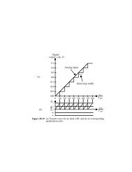
Infinite Mass <strong>Opening</strong> <strong>Shock</strong><br />
Factor<br />
• Wind tunnel data for<br />
models with only<br />
geometric porosity<br />
variations<br />
• Disreefed from nearly<br />
closed to full open in<br />
steady flow<br />
• High opening shock<br />
the result of faster<br />
inflation at low<br />
porosities<br />
<strong>Parachute</strong> <strong>Inflation</strong> <strong>and</strong> <strong>Opening</strong> 13
Finite Mass <strong>Opening</strong> <strong>Shock</strong> Factor<br />
• Finite mass opening shock factor is primarily a function of<br />
mass ratio (characteristic fluid mass/system mass)<br />
– Inverse ratio (system mass/characteristic fluid mass) also<br />
sometimes used<br />
• Most common mass ratio used is [ρ(CdS) 1.5 /M ]<br />
– Where ρ is atmospheric density<br />
– CdS is parachute drag area<br />
– M is system mass<br />
• Most extensive correlations<br />
– Ewing AFFDL-TR-72-3<br />
– Knacke NWC TP 6575<br />
<strong>Parachute</strong> <strong>Inflation</strong> <strong>and</strong> <strong>Opening</strong> 14
Finite Mass <strong>Opening</strong> <strong>Shock</strong> Factor<br />
• For unreefed<br />
parachute or<br />
inflation to 1 st<br />
reefed stage<br />
• Data from other<br />
sources added to<br />
Knacke/Ewing data<br />
• Data near Y-axis<br />
from infinite mass<br />
wind tunnel tests<br />
<strong>Parachute</strong> <strong>Inflation</strong> <strong>and</strong> <strong>Opening</strong> 15
Finite Mass <strong>Opening</strong> <strong>Shock</strong> Factor<br />
• For disreef of<br />
reefed parachute<br />
• Data from other<br />
sources added to<br />
Knacke/Ewing data<br />
• Data near Y-axis<br />
from infinite mass<br />
wind tunnel tests<br />
<strong>Parachute</strong> <strong>Inflation</strong> <strong>and</strong> <strong>Opening</strong> 16
Finite Mass <strong>Opening</strong> <strong>Shock</strong> Factor<br />
• Ewing/Bixby/Knacke<br />
AFFL-TR-78-151<br />
• Same data set as<br />
Knacke/Ewing data<br />
• More specific data<br />
correlations from<br />
subsets of the data<br />
• Extremes of data<br />
scatter shown with<br />
mean values<br />
<strong>Parachute</strong> <strong>Inflation</strong> <strong>and</strong> <strong>Opening</strong> 17
<strong>Parachute</strong> Load Estimates<br />
• Finite mass opening shock factors can be used to<br />
provide rapid estimates of parachute opening<br />
loads<br />
– No computer code required<br />
– Calculator or “back of the envelope” estimate<br />
– Might need atmosphere table<br />
– Accurate enough for most parachute design work<br />
– Quick “sanity check” for computer codes<br />
<strong>Parachute</strong> <strong>Inflation</strong> <strong>and</strong> <strong>Opening</strong> 18
Unsteady Flow Equation<br />
• Bernoulli equation for unsteady,<br />
inviscid, incompressible <strong>and</strong><br />
irrotational flow along a streamline<br />
(perfect fluid)<br />
P 1 2 ∂φ<br />
+ V + = C(t)<br />
ρ<br />
2<br />
∂t<br />
– φ = velocity potential (grad φ = V)<br />
– t = time<br />
<strong>Parachute</strong> <strong>Inflation</strong> <strong>and</strong> <strong>Opening</strong> 19
Unsteady Flow Around Sphere<br />
• Pressure distribution on a sphere in<br />
unsteady, inviscid, incompressible<br />
<strong>and</strong> irrotational flow along a<br />
streamline (perfect fluid)<br />
P ∞ 2<br />
V + Rcos<br />
θ<br />
-P<br />
⎛ 9 2 5<br />
⎞<br />
= ⎜ cos θ - ⎟<br />
ρ ⎝ 8 8 ⎠<br />
– R = radius of sphere<br />
1<br />
2<br />
∂V<br />
∂t<br />
<strong>Parachute</strong> <strong>Inflation</strong> <strong>and</strong> <strong>Opening</strong> 20
Unsteady Flow Kinetic Energy<br />
• For the same unsteady flow (unsteady,<br />
inviscid, incompressible, irrotational),<br />
the fluid kinetic energy can be written<br />
T =<br />
1<br />
2<br />
2<br />
A x Vx<br />
– T = kinetic energy<br />
– Ax = a fluid mass<br />
– Vx = velocity of fluid mass ( body)<br />
<strong>Parachute</strong> <strong>Inflation</strong> <strong>and</strong> <strong>Opening</strong> 21
Unsteady Flow Force<br />
• The unsteady fluid force on a body in onedimensional<br />
motion is<br />
F<br />
x<br />
=<br />
−<br />
d<br />
dt<br />
⎛ ∂T<br />
⎜<br />
⎝ ∂V<br />
dV<br />
dt<br />
• For a sphere, A x can be written<br />
x<br />
⎞<br />
⎟<br />
⎠<br />
Cax = 0.5 (apparent mass coefficient)<br />
Rp = parachute radius<br />
=<br />
−<br />
A<br />
4<br />
A x =<br />
Cax<br />
ρ π R<br />
3<br />
x<br />
3<br />
p<br />
x<br />
<strong>Parachute</strong> <strong>Inflation</strong> <strong>and</strong> <strong>Opening</strong> 22
Ballistic Equations of Motion<br />
• The equations of motion used in most simple trajectory<br />
computer codes are the ballistic or zero angle of attack<br />
equations<br />
dV<br />
dt<br />
x<br />
2<br />
( m + A ) = m g sin γ - C ρ V S<br />
x<br />
dγ<br />
dt<br />
( +<br />
A ) V = m g cos γ<br />
m x x<br />
m = system mass<br />
g = gravitational acceleration<br />
γ = trajectory angle<br />
d<br />
1<br />
2<br />
<strong>Parachute</strong> <strong>Inflation</strong> <strong>and</strong> <strong>Opening</strong> 23<br />
x
Dimensionless Equations<br />
• The ballistic equations can be written in<br />
dimensionless form<br />
dV<br />
dt *<br />
x*<br />
=<br />
dγ<br />
= *<br />
dt<br />
F<br />
r<br />
sin γ<br />
⎛<br />
⎜<br />
⎜1<br />
+<br />
⎝<br />
K<br />
F V<br />
r<br />
x*<br />
t<br />
C<br />
K<br />
ax<br />
t<br />
⎞<br />
⎟<br />
⎠<br />
cos γ<br />
−<br />
( K + C )<br />
t<br />
ax<br />
3<br />
8<br />
( K + C )<br />
t<br />
C<br />
<strong>Parachute</strong> <strong>Inflation</strong> <strong>and</strong> <strong>Opening</strong> 24<br />
d<br />
V<br />
2<br />
x<br />
ax
Dimensionless Variables <strong>and</strong><br />
Parameters<br />
• Dimensionless Variables<br />
V<br />
x V x*<br />
= ; t * =<br />
V0<br />
• Dimensionless Parameters<br />
F<br />
r<br />
2<br />
V0<br />
= ;<br />
gR<br />
V 0 = initial velocity<br />
p<br />
K<br />
t<br />
=<br />
t V<br />
R<br />
p<br />
0<br />
m<br />
4<br />
ρ π<br />
3<br />
R<br />
3<br />
p<br />
<strong>Parachute</strong> <strong>Inflation</strong> <strong>and</strong> <strong>Opening</strong> 25
Unsteady Flow Around Exp<strong>and</strong>ing<br />
Decelerating Sphere<br />
• Pressure distribution on an exp<strong>and</strong>ing,<br />
decelerating sphere in inviscid,<br />
incompressible <strong>and</strong> irrotational flow<br />
P - P∞<br />
⎛ 9 2 5 ⎞ 2 1 dVx<br />
= ⎜ cos θ − ⎟ Vx<br />
+ Rcos<br />
θ<br />
ρ ⎝ 8 8 ⎠ 2 dt<br />
V r =<br />
+<br />
3<br />
2<br />
dR<br />
dt<br />
V<br />
2<br />
r<br />
dVr<br />
+ R<br />
dt<br />
+<br />
3<br />
2<br />
cosθ<br />
V<br />
<strong>Parachute</strong> <strong>Inflation</strong> <strong>and</strong> <strong>Opening</strong> 26<br />
x<br />
V<br />
r
Unsteady Forces on Inflating,<br />
Decelerating <strong>Parachute</strong><br />
• Axial force along flight path<br />
F<br />
xu<br />
=<br />
−<br />
⎛<br />
⎜<br />
⎝<br />
• Radial force<br />
Fru<br />
=<br />
⎛<br />
− ⎜ A<br />
⎝<br />
dV<br />
dt<br />
• No axial/radial coupling<br />
A<br />
x<br />
r<br />
x<br />
dV<br />
dt<br />
r<br />
+<br />
+<br />
V<br />
x<br />
V<br />
r<br />
dA<br />
dt<br />
x<br />
dA<br />
dt<br />
r<br />
⎞<br />
⎟<br />
⎠<br />
⎞<br />
⎟<br />
⎠<br />
<strong>Parachute</strong> <strong>Inflation</strong> <strong>and</strong> <strong>Opening</strong> 27
Dimensional Analysis <strong>and</strong> Unsteady<br />
Flow Conclusions<br />
• Dimensional analysis identifies dimensionless<br />
parameters that influence opening shock <strong>and</strong><br />
inflation time<br />
– Mass ratio Kt = m / [(4/3) ρπR 3<br />
p ]<br />
– Froude number Fr = V 2<br />
0 / (g Rp)<br />
• Simplified perfect fluid analysis provides insight<br />
into functional form of forces <strong>and</strong> pressure<br />
distributions<br />
<strong>Parachute</strong> <strong>Inflation</strong> <strong>and</strong> <strong>Opening</strong> 28
Drag Area vs Time <strong>Inflation</strong> Models<br />
• Simplest models specified drag area vs time as<br />
input to a point mass trajectory code<br />
– <strong>Inflation</strong> times often artificially adjusted to match loads<br />
– <strong>Inflation</strong> times sometimes scaled using dimensionless<br />
time<br />
• Use of drag area as an independent variable in<br />
trajectory codes explains use of drag area<br />
directly to calculate mass ratio<br />
• Combined use of point mass computer code <strong>and</strong><br />
the mass ratio C k correlations improved use of<br />
this method<br />
<strong>Parachute</strong> <strong>Inflation</strong> <strong>and</strong> <strong>Opening</strong> 29
Continuity Equation <strong>Inflation</strong> Models<br />
• More sophisticated models solved a conservation<br />
of mass equation for the parachute internal<br />
volume<br />
– Mass flow in determines rate of change of internal<br />
volume<br />
– Similar shapes used to get diameter <strong>and</strong> parachute drag<br />
• Calculated shapes combined with point mass<br />
trajectory code<br />
– Apparent mass often used in equations of motion<br />
• Extensive work by U. of Minnesota – Dr. Heinrich<br />
<strong>Parachute</strong> <strong>Inflation</strong> <strong>and</strong> <strong>Opening</strong> 30
Similar Shapes Used in Continuity<br />
Equation <strong>Inflation</strong> Models<br />
• Early shapes were<br />
simple because<br />
calculations were<br />
manual<br />
• More realistic<br />
shapes allowed<br />
using computers<br />
• Inflow <strong>and</strong> outflow<br />
assumptions<br />
required<br />
<strong>Parachute</strong> <strong>Inflation</strong> <strong>and</strong> <strong>Opening</strong> 31
Constant Distance Theory Models<br />
• Another family of inflation models was<br />
based on the observation that “a<br />
parachute always inflates in a fixed<br />
distance traveled”<br />
• This assumption is equivalent to the<br />
conservation of mass assumption<br />
– A column of air ahead of the parachute<br />
eventually occupies the internal volume<br />
<strong>Parachute</strong> <strong>Inflation</strong> <strong>and</strong> <strong>Opening</strong> 32
Constant Distance Theory Models<br />
• Both the conservation of mass <strong>and</strong><br />
constant distance theory models assume<br />
dynamic similarity in the inflation process<br />
– <strong>Parachute</strong> mass ratio doesn’t change much<br />
• Instead of similar shapes, radial velocity<br />
can be directly specified to be a function<br />
of axial velocity<br />
• A compressibility correction to constant<br />
distance theory was proposed<br />
<strong>Parachute</strong> <strong>Inflation</strong> <strong>and</strong> <strong>Opening</strong> 33
Proposed Compressibility Correction<br />
• Compressibility<br />
correction assumed<br />
normal shock ahead<br />
of canopy for density<br />
correction<br />
• Wind tunnel photo<br />
<strong>and</strong> drag data show<br />
this is incorrect<br />
– Actual density change<br />
is small fraction of<br />
normal shock<br />
correction<br />
<strong>Parachute</strong> <strong>Inflation</strong> <strong>and</strong> <strong>Opening</strong> 34
Simple Dynamic <strong>Inflation</strong> Model<br />
• Model based on conservation of<br />
momentum<br />
– <strong>Parachute</strong> inflation is a dynamics<br />
problem, not a quasi-static problem<br />
– Single radial degree of freedom<br />
– Rigid coupling parachute <strong>and</strong> payload<br />
– Unreefed parachutes only<br />
– Steady <strong>and</strong> unsteady aerodynamic<br />
effects<br />
<strong>Parachute</strong> <strong>Inflation</strong> <strong>and</strong> <strong>Opening</strong> 35
Trajectory for Model<br />
• Ballistic (zero<br />
angle of attack)<br />
trajectory<br />
• Velocity at payload<br />
<strong>and</strong> parachute<br />
different because<br />
parachute moves<br />
toward payload<br />
during inflation<br />
<strong>Parachute</strong> <strong>Inflation</strong> <strong>and</strong> <strong>Opening</strong> 36
<strong>Parachute</strong> Geometry for Model<br />
• Similar shapes<br />
– Hemispherical<br />
inflated part<br />
– Conical uninflated<br />
part<br />
• Rigid coupling<br />
between parachute<br />
<strong>and</strong> payload<br />
<strong>Parachute</strong> <strong>Inflation</strong> <strong>and</strong> <strong>Opening</strong> 37
Simple Dynamic <strong>Inflation</strong> Model<br />
• Single canopy mass element located<br />
at maximum diameter point<br />
• Steady radial force coefficient data<br />
based on inflated geometry<br />
• Radial force to drag force ratio<br />
required to produce canopy shape<br />
was obtained from photographic data<br />
<strong>Parachute</strong> <strong>Inflation</strong> <strong>and</strong> <strong>Opening</strong> 38
Simple Dynamic <strong>Inflation</strong> Model<br />
• Equations were put in non-dimensional<br />
form<br />
– A second mass ratio, the parachute mass ratio,<br />
was revealed<br />
• Predictions of the model were compared<br />
with test data from the PEPP tests<br />
• Predicted inflation time variations over the<br />
wide altitude range of tests agreed very<br />
well with PEPP data<br />
<strong>Parachute</strong> <strong>Inflation</strong> <strong>and</strong> <strong>Opening</strong> 39
Non-dimentional <strong>Inflation</strong> Times for<br />
DGB <strong>Parachute</strong>s<br />
• Dimensionless<br />
inflation times<br />
correlated well<br />
with parachute<br />
mass ratio over<br />
wide altitude range<br />
• No compressibility<br />
correction<br />
<strong>Parachute</strong> <strong>Inflation</strong> <strong>and</strong> <strong>Opening</strong> 40
Non-dimentional <strong>Inflation</strong> Times for all<br />
PEPP <strong>Parachute</strong>s<br />
• Dimensionless<br />
inflation times<br />
correlated well<br />
with lower bound<br />
of data<br />
• No compressibility<br />
correction<br />
<strong>Parachute</strong> <strong>Inflation</strong> <strong>and</strong> <strong>Opening</strong> 41
Non-dimentional <strong>Inflation</strong> Times for all<br />
PEPP <strong>Parachute</strong>s<br />
• Dimensionless<br />
inflation times with<br />
compressibility<br />
corrections based<br />
on density<br />
estimate required<br />
for drag coefficient<br />
vs Mach number<br />
variation<br />
<strong>Parachute</strong> <strong>Inflation</strong> <strong>and</strong> <strong>Opening</strong> 42
<strong>Opening</strong> <strong>Shock</strong> Factor for all PEPP<br />
<strong>Parachute</strong>s<br />
• Drag coefficient vs<br />
Mach number from<br />
wind tunnel data<br />
• Predictions span<br />
range of data<br />
scatter<br />
<strong>Parachute</strong> <strong>Inflation</strong> <strong>and</strong> <strong>Opening</strong> 43
Conclusions from Simple Dynamic<br />
<strong>Inflation</strong> Model Study<br />
• <strong>Parachute</strong> mass ratio should be<br />
considered an important scaling<br />
factor for use of parachutes in low<br />
density environment<br />
• Compressibility correction appears<br />
to be much less than proposed for<br />
constant distance theory models<br />
<strong>Parachute</strong> <strong>Inflation</strong> <strong>and</strong> <strong>Opening</strong> 44
More General Dynamic <strong>Inflation</strong> Model<br />
• Two radial degrees of freedom<br />
• Elastic elements couple parachute<br />
masses <strong>and</strong> payload<br />
• Can be used to model reefed<br />
parachutes<br />
• Parametric aerodynamic data for<br />
different porosities measured to<br />
provide design data base<br />
<strong>Parachute</strong> <strong>Inflation</strong> <strong>and</strong> <strong>Opening</strong> 45
Trajectory for Model<br />
• Ballistic (zero<br />
angle of attack)<br />
trajectory<br />
• Velocity at payload<br />
<strong>and</strong> parachute<br />
different because<br />
parachute moves<br />
toward payload<br />
during inflation<br />
<strong>Parachute</strong> <strong>Inflation</strong> <strong>and</strong> <strong>Opening</strong> 46
Forces on Mass Elements<br />
• Two parachute<br />
mass elements<br />
– Maximum diameter<br />
– Skirt<br />
• Radial force<br />
applied at<br />
maximum diameter<br />
element<br />
<strong>Parachute</strong> <strong>Inflation</strong> <strong>and</strong> <strong>Opening</strong> 47
Elastic Constraints on Mass<br />
Elements<br />
• Allows different<br />
elastic properties<br />
for suspension<br />
lines <strong>and</strong> radials<br />
• Realistic modeling<br />
of reefing line<br />
constraint <strong>and</strong><br />
cutting of reefing<br />
line<br />
<strong>Parachute</strong> <strong>Inflation</strong> <strong>and</strong> <strong>Opening</strong> 48
Use of Dynamic <strong>Inflation</strong> Model<br />
• Used to design<br />
many parachutes<br />
at S<strong>and</strong>ia<br />
• Reefing easy to<br />
include<br />
• Also used to study<br />
wake overtake<br />
which occurs<br />
during rapid<br />
deceleration<br />
<strong>Parachute</strong> <strong>Inflation</strong> <strong>and</strong> <strong>Opening</strong> 49
Multi-Element Dynamic <strong>Inflation</strong><br />
Model<br />
• Many mass<br />
elements used to<br />
model parachute<br />
• Used to study<br />
parachute<br />
deployment <strong>and</strong><br />
inflation in greater<br />
detail<br />
<strong>Parachute</strong> <strong>Inflation</strong> <strong>and</strong> <strong>Opening</strong> 50
Multi-Element Dynamic <strong>Inflation</strong><br />
Model<br />
• Used to study<br />
variations of<br />
tension, radius,<br />
pressure <strong>and</strong> other<br />
variables along<br />
length of<br />
parachute<br />
<strong>Parachute</strong> <strong>Inflation</strong> <strong>and</strong> <strong>Opening</strong> 51
<strong>Parachute</strong> <strong>Inflation</strong> <strong>and</strong> <strong>Opening</strong> 52
<strong>Parachute</strong> <strong>Inflation</strong> <strong>and</strong> <strong>Opening</strong> 53