PyMca, Hyperspectral Data and HDF5 - ESRF
PyMca, Hyperspectral Data and HDF5 - ESRF
PyMca, Hyperspectral Data and HDF5 - ESRF

You also want an ePaper? Increase the reach of your titles
YUMPU automatically turns print PDFs into web optimized ePapers that Google loves.
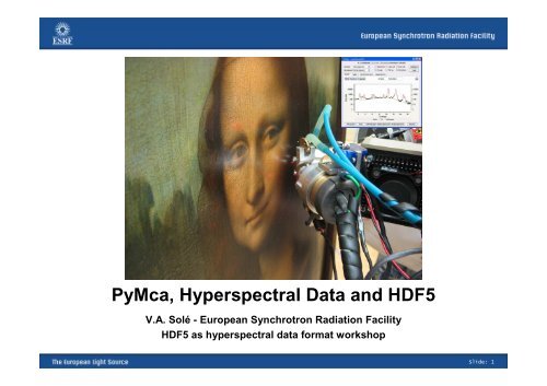
<strong>PyMca</strong>, <strong>Hyperspectral</strong> <strong>Data</strong> <strong>and</strong> <strong>HDF5</strong><br />
V.A. Solé - European Synchrotron Radiation Facility<br />
<strong>HDF5</strong> as hyperspectral data format workshop<br />
Slide: 1
<strong>PyMca</strong>?<br />
<strong>PyMca</strong> is set of software tools mostly known in the field of XRF analysis<br />
It is certainly a set of programs <strong>and</strong> widgets for XRF analysis:<br />
Spectrum modeling<br />
Quantification<br />
ROI imaging<br />
Fit imaging via batch processing<br />
But also a set of programs <strong>and</strong> generic python modules for:<br />
<strong>Data</strong> visualization<br />
Peak search<br />
Function fitting<br />
Imaging of stacked data<br />
V.A. Solé, E. Papillon, M. Cotte, Ph. Walter, J. Susini, Spectrochimica Acta B 62 (2007) 63-68<br />
Slide: 2
Integration into our acquisition system<br />
Slide: 3
Free distribution<br />
Slide: 4
Multiplatform<br />
Slide: 5
Multiplatform<br />
Slide: 6
<strong>PyMca</strong> Visualization<br />
<strong>Data</strong> courtesy of P. Cloetens<br />
<strong>PyMca</strong> <strong>PyMca</strong> Object3D Object3D Module<br />
Module<br />
Up Up Up to to 4D 4D visualization<br />
visualization<br />
<strong>Data</strong> courtesy of A. Díaz<br />
<strong>Data</strong> courtesy of J.A. Sans <strong>and</strong> G. Martínez<br />
Slide: 7
Complete M-shell support<br />
Slide: 8
Use of (sub-)shell mass attenuation coefficients<br />
Direct photoelectric ionization of the i (sub-)shell:<br />
( E, i)<br />
( E)<br />
⎛τ ⎞<br />
⎜<br />
⎝ τ ⎟<br />
⎠<br />
( )<br />
i<br />
Pi ∝ ⎜ ⎟τ<br />
E<br />
<strong>PyMca</strong> versus<br />
Term between parenthesis for Pb<br />
Energy 16 keV 20 keV 25 keV 30 keV<br />
L1 0.136 0.164 0.192 0.218<br />
L2 0.248 0.247 0.244 0.240<br />
L3 0.367 0.345 0.323 0.303<br />
Ji<br />
−1<br />
Pi ∝ τ E<br />
J<br />
A. Brunetti, M. Sánchez del Río, B. Golosio, A. Simionovici, A. Somogyi, Spectrochimica Acta B 59 (2004) 1725-1731<br />
i<br />
( )<br />
J.H. Scofield. Theor. Photo. Cross Sections from 1 to 1500 keV, LLNL Report UCRL-51326, Livermore, Ca 1973.<br />
Slide: 9
De-excitation cascade taken into account<br />
<strong>PyMca</strong> considers the vacancies produced in an atomic shell or sub-shell by<br />
the de-excitation process of an inner shell or sub-shell.<br />
Radiative <strong>and</strong> Coster-Kronig transitions correctly considered.<br />
Auger transitions approximated.<br />
Slide: 10
XRF Spectrum Analysis<br />
Typical procedure:<br />
1. Calibration<br />
2. Peak identification<br />
3. Peak area extraction<br />
Region of interest (ROI)<br />
Deconvolution (FIT)<br />
4. Quantification<br />
Documentation at http://pymca.sourceforge.net/documentation.html<br />
Slide: 11
Fit configuration Dialog (I)<br />
Slide: 12
Fit Configuration Dialog (II)<br />
Slide: 13
Quantification (I)<br />
Parallel Parallel beam beam approximation<br />
approximation<br />
Slide: 14
Quantification (II)<br />
Nominal concentration 500 ppm<br />
Slide: 15
XRF Analysis Integration in other Applications<br />
Integration in mxCuBE (<strong>ESRF</strong>) Integration elsewhere<br />
Slide: 16
Is it easy to embed?<br />
For the previous examples, basically one just needs 4 lines of code:<br />
from <strong>PyMca</strong> import McaAdvancedFit<br />
fitWindow = McaAdvancedFit.McaAdvancedFit()<br />
fitWindow.set<strong>Data</strong>(x, y)<br />
fitWindow.show()<br />
It can be used interactively from ipython just starting it as “ipython –q4thread”<br />
Slide: 17
One spectrum for each pixel<br />
…<br />
…<br />
+<br />
A sum spectrum for the whole image<br />
XRF Imaging<br />
Slide: 18
Advanced Fit Batch processing<br />
Select the input files<br />
Select the fit configuration<br />
Select the output directory<br />
Select the output options<br />
Start<br />
Slide: 19
Images in ASCII <strong>and</strong> <strong>ESRF</strong> format<br />
• Easy to import in other programs<br />
Individual peak contributions in ASCII<br />
• Use your own plotting program<br />
Fully automated HTML report<br />
• Browse your results!<br />
Output<br />
Slide: 20
Copyright C2RMF<br />
S<br />
Pb<br />
Ca<br />
Sb<br />
We wanted to know what pigments were<br />
used in this section of the painting<br />
Slide: 21
Based on the batch generated element distribution maps …<br />
Slide: 22
… <strong>and</strong> their correlations as shown by the program<br />
Sulfur <strong>and</strong> antimony correlated Lead <strong>and</strong> antimony not correlated<br />
… we were able to determine the possible presence of stibnite grains (Sb 2 S 3 )<br />
embedded in a lead containing matrix.<br />
M. Cotte, E. Welcomme, V.A. Solé, M. Salomé, M. Menu, Ph. Walter, J. Susini, Anal. Chem. 79 (2007) 6988-6994<br />
Slide: 23
Stack ROI Imaging<br />
In this example:<br />
Stack = 101x200x2000 numpy array<br />
20200 spectra of 2000 channels<br />
Pixel[i, j] = numpy.sum(Stack[i, j, :])<br />
Pixel[i, j] = numpy.sum(Stack[i, j, ch0:ch1])<br />
We can generate new images by moving the cursors or defining new ROIs in the table<br />
Slide: 24
Eigenimages <strong>and</strong> Eigenvectors<br />
Slide: 25
Eigenimages <strong>and</strong> Eigenvectors<br />
Slide: 26
Eigenimages <strong>and</strong> Eigenvectors<br />
Slide: 27
Eigenimages <strong>and</strong> Eigenvectors<br />
Slide: 28
Eigenimages <strong>and</strong> Eigenvectors<br />
Slide: 29
Eigenimages <strong>and</strong> Eigenvectors<br />
Slide: 30
Getting the actual information<br />
We can select a set of pixels on any of<br />
the displayed images <strong>and</strong> display the<br />
cumulative spectrum associated to those<br />
pixels.<br />
Here we can see the average spectrum<br />
associated to the hotter pixels of the<br />
Eigenimage 02 (in red) compared to the<br />
average spectrum of the map (in black).<br />
Slide: 31
We could have easily missed the<br />
presence of one element if we would<br />
have just analyzed the sum spectrum<br />
via ROIs.<br />
Slide: 32
What have we done?<br />
We have used multivariate analysis (PCA in this case) to know what sample regions<br />
were worth to take a closer look.<br />
Not bad when you have a lot of data …<br />
This This data data treatment treatment is is totally totally generic generic <strong>and</strong> <strong>and</strong> applicable applicable to to other other techniques<br />
t<br />
echniques<br />
Slide: 33
Multivariate Analysis Capabilities<br />
<strong>PyMca</strong> makes use of PCA, ICA (via MDP toolkit) <strong>and</strong> NNMA (via py_nnma)<br />
For the time being, multivariate analysis is used just to identify sample regions with<br />
different properties. The associated physical spectrum gives the actual information.<br />
It can combine information from different simultaneously acquired datasets, for<br />
instance XRD <strong>and</strong> XRF data or PIXE <strong>and</strong> RBS.<br />
Slide: 34
<strong>PyMca</strong> <strong>HDF5</strong>/NeXus<br />
SOLEIL NeXus <strong>Data</strong> courtesy of J.A. Sans <strong>and</strong> G. Martínez<br />
<strong>HDF5</strong> <strong>HDF5</strong> Support<br />
Support<br />
Collaboration Collaboration with with with D. D. D. Dale, Dale, Dale, CHESS<br />
CHESS<br />
Slide: 35
Generic <strong>HDF5</strong> Visualization<br />
Generic: Select what to plot, how to plot it, <strong>and</strong> plot it.<br />
Slide: 36
The <strong>PyMca</strong> <strong>HDF5</strong> problem<br />
<strong>PyMca</strong> can do a lot more than “just” fully analyze XRF spectra<br />
<strong>PyMca</strong> can read <strong>HDF5</strong> data … but often has no clue about what to do without asking<br />
Properly defined NXdata groups can provide default visualization <strong>and</strong> more<br />
It would be great to automatically identify the different MCA detectors, with their<br />
counts, their energy axis, their preset time, their elapsed time, their calibration, …<br />
NeXus NXdetector has almost everything needed to describe an MCA, but still needs<br />
user interaction to know that detector is an MCA.<br />
It would be very simple to add two attributes to datasets. One defining the “natural”<br />
data dimensions <strong>and</strong> other one defining those dimensions are the first or the last<br />
ones of the dataset.<br />
Slide: 37
What can two attributes bring?<br />
Programs would automatically provide better user choices<br />
Programs would know what to do with datasets! Despite being able to perform 4D<br />
plots, <strong>PyMca</strong> does not know (it could just guess) what to do to visualize datasets<br />
with dimensions 1 x 2 x 512 x 1024.<br />
One attribute to say “ACTUAL_DIMENSION = 2”<br />
One attribute to say “ACTUAL_DIMENSION_IS_LAST_DIMENSION = 1”<br />
And things are totally different than:<br />
One attribute to say “ACTUAL_DIMENSION = 1”<br />
One attribute to say “ACTUAL_DIMENSION_IS_LAST_DIMENSION = 1”<br />
Slide: 38
The alternative looks ugly, doesn’t it?<br />
Just imagine a wall made of buttons instead of bricks everywhere ….<br />
Slide: 39
<strong>PyMca</strong> is a program as well as a toolkit<br />
Conclusion<br />
- Open source <strong>and</strong> distributed under the conditions of the GPLv2+<br />
- Supports <strong>HDF5</strong> among other formats<br />
- Can be used as a multivariate analysis tool<br />
- Can be used as a fitting <strong>and</strong> visualization tool (for up to 4-dimensional data)<br />
- Allows you to specify a physically meaningful model which can quantitatively<br />
determine element concentrations from energy dispersive X-ray spectra<br />
- Provides high level widgets based on PyQt that can be used independently or<br />
integrated into your application<br />
- Has an active development funded by the <strong>ESRF</strong><br />
Slide: 40
Acknowledgements<br />
My <strong>ESRF</strong> colleagues (mainly software group <strong>and</strong> microscopy beamlines ID21 <strong>and</strong> ID22)<br />
Ph. Walter <strong>and</strong> coworkers from the Centre de Recherche et de Restauration des Musées<br />
de France<br />
Darren Dale (Cornell High Energy Synchrotron Source)<br />
The community of Python developers of free software<br />
The <strong>PyMca</strong> users, for their enthusiasm <strong>and</strong> their encouragements<br />
Slide: 41