Santa Clara River Estuary Annual Report 2005 - City Of Ventura
Santa Clara River Estuary Annual Report 2005 - City Of Ventura
Santa Clara River Estuary Annual Report 2005 - City Of Ventura

Create successful ePaper yourself
Turn your PDF publications into a flip-book with our unique Google optimized e-Paper software.
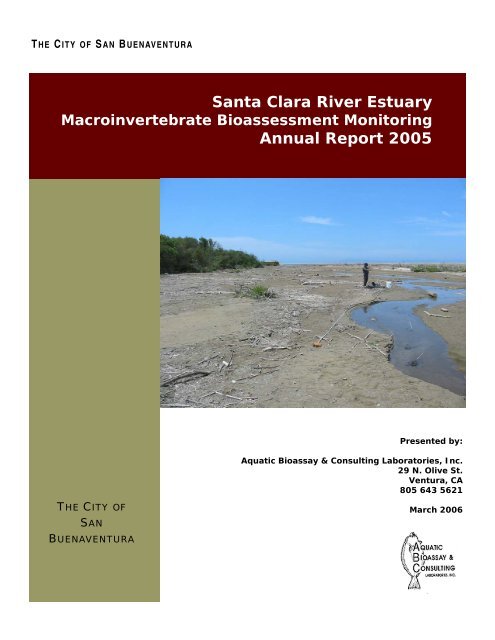
T HE CITY OF SAN BUENAVENTURA<br />
<strong>Santa</strong> <strong>Clara</strong> <strong>River</strong> <strong>Estuary</strong><br />
Macroinvertebrate Bioassessment Monitoring<br />
<strong>Annual</strong> <strong>Report</strong> <strong>2005</strong><br />
THE CITY OF<br />
SAN<br />
BUENAVENTURA<br />
Presented by:<br />
Aquatic Bioassay & Consulting Laboratories, Inc.<br />
29 N. Olive St.<br />
<strong>Ventura</strong>, CA<br />
805 643 5621<br />
March 2006
<strong>City</strong> of San Buenaventura<br />
<strong>Santa</strong> <strong>Clara</strong> <strong>River</strong> <strong>Estuary</strong> Monitoring <strong>Report</strong> <strong>2005</strong><br />
TABLE OF CONTENTS<br />
INTRODUCTION ................................................................................................. 2<br />
Site Description........................................................................................... 2<br />
Bioassessment Monitoring ............................................................................ 3<br />
MATERIALS AND METHODS .................................................................................... 5<br />
Field Methods ............................................................................................. 5<br />
Laboratory Methods..................................................................................... 6<br />
Sample Processing.................................................................................... 6<br />
QA/QC .................................................................................................... 7<br />
Particle Size Analysis ................................................................................... 7<br />
Data Analysis.............................................................................................. 8<br />
Multi-metric analysis ................................................................................. 8<br />
Univariate and Multivariate Analysis ...........................................................10<br />
RESULTS .......................................................................................................11<br />
<strong>Annual</strong> Stream Flow & <strong>Estuary</strong> Inundation .....................................................11<br />
General Observations..................................................................................13<br />
Physical Measurements and Water Quality .....................................................13<br />
May .......................................................................................................13<br />
October..................................................................................................13<br />
Sediment Particle Size ................................................................................15<br />
Macrobenthic Invertebrates .........................................................................17<br />
Summary ...............................................................................................17<br />
Bioassessment Metrics .............................................................................17<br />
Most Abundant Species ............................................................................23<br />
Cluster Analysis.......................................................................................25<br />
DISCUSSION ...................................................................................................27<br />
APPENDIX A - REFERENCES ..................................................................................31<br />
General references .....................................................................................31<br />
Taxonomic identification resources used ........................................................32<br />
APPENDIX B – SEDIMENT PARTICLE SIZE ..................................................................34<br />
APPENDIX C - MACROINVERTEBRATES ......................................................................36
<strong>City</strong> of San Buenaventura<br />
<strong>Santa</strong> <strong>Clara</strong> <strong>River</strong> <strong>Estuary</strong> Monitoring <strong>Report</strong> <strong>2005</strong><br />
INTRODUCTION<br />
This report is submitted in fulfillment of<br />
the <strong>City</strong> of San Buenaventura’s<br />
bioassessment monitoring portion of<br />
National Pollutant Elimination Discharge<br />
System (NPDES) permit No.<br />
CA0052651 (Order No. 00-143). The<br />
<strong>City</strong> owns and operates the <strong>Ventura</strong><br />
Water Reclamation Facility (VWRF)<br />
adjacent to the north edge of the <strong>Santa</strong><br />
<strong>Clara</strong> <strong>River</strong> <strong>Estuary</strong> (SCRE). The VWRF<br />
discharges tertiary treated effluent into<br />
the <strong>Estuary</strong> at a relatively constant rate<br />
of between 7 and 10 million gallons<br />
each day. The monitoring program described herein was developed based on several<br />
past studies of the <strong>Estuary</strong> (Engineering Science 1976; Swanson 1990; USFWS<br />
1999; ENTRIX 1999, 2002 and 2003; Aquatic Bioassay 2004 and <strong>2005</strong>).<br />
The main objective of this program is to assess if the effluent emanating from the<br />
VWRF is impacting the populations of organisms living in the SCRE, taking into<br />
account the influence of both physical habitat and seasonal differences between<br />
sampling locations. Potential impacts would include differences in the abundance,<br />
diversity and/or composition of organisms residing in the effluent channel (Stations<br />
B1 and B2) versus those located in the lower estuary (Station B3) and in the main<br />
river channels (Station B7).<br />
To address this objective, Aquatic Bioassay & Consulting Laboratories scientists<br />
conducted bioassessment monitoring of the <strong>Santa</strong> <strong>Clara</strong> <strong>River</strong> <strong>Estuary</strong> during both<br />
the spring and fall of <strong>2005</strong>, in accordance with the <strong>City</strong>’s NPDES permit and the<br />
California Stream Bioassessment Protocol (CSBP 2003). The methods, findings and<br />
discussion of these surveys are presented in this report.<br />
Site Description<br />
The <strong>Santa</strong> <strong>Clara</strong> <strong>River</strong> is the longest free-flowing river in southern California. Its 70<br />
mile length provides drainage to a 1,600 mi 2 watershed. Flow in the river typically<br />
reaches 100,000 cubic feet per second (cfs) during winter and spring storm flows<br />
(Swanson et al. 1990). The SCRE is located at the mouth of the river and is<br />
characterized as a typical river mouth estuary (Ferran 1989, Ferran et al. 1996). The<br />
<strong>Estuary</strong> is a highly dynamic environment due to hydrology patterns that can vary<br />
greatly during the year. The flow of water into the SCRE is influenced by dry and wet<br />
weather flow from the <strong>Santa</strong> <strong>Clara</strong> <strong>River</strong>, Pacific Ocean tides and the effluent<br />
emanating from the <strong>City</strong> of San Buenaventura’s, <strong>Ventura</strong> Water Reclamation Facility<br />
(VWRF). During the winter and spring, the river is open to the ocean due to sandbarbreaching<br />
storm flows. During the summer and fall the sandbar becomes well<br />
established due to lack of rainfall, low river flow and small summer surf. Once<br />
established, the berm creates a barrier to flow and allows the <strong>Estuary</strong> to become<br />
inundated with water from the VWRF. Depth of the estuary during peak inundation<br />
can reach nearly 10 ft above Mean Sea Level (MSL) (USFWS 1999).<br />
In 1855, the <strong>Estuary</strong> was estimated to have encompassed 870 acres (Swanson et al.<br />
1990, State Coastal Conservancy et al. 1997), but its size has declined to its present<br />
160 acres, due to the diversion of upstream river flow to municipal water projects<br />
2
<strong>City</strong> of San Buenaventura<br />
<strong>Santa</strong> <strong>Clara</strong> <strong>River</strong> <strong>Estuary</strong> Monitoring <strong>Report</strong> <strong>2005</strong><br />
and agriculture (ENTRIX 2002). This reduction in flow has, in part, been replaced by<br />
the relatively constant flow of tertiary treated effluent (7 to 10 MGD) from the VWRF.<br />
The tertiary treatment process creates effluent essentially free of organics and is<br />
very low in nutrients. This flow provides a water source to the <strong>Estuary</strong> during periods<br />
when it would otherwise be dry. Since most southern California estuaries experience<br />
drought during the summer and fall (Zedler 1982), this has created a unique, low<br />
salinity habitat for a wide array of aquatic organisms, water birds and other<br />
vertebrates. The lack of understanding regarding the relationship between the<br />
biological resources found in the estuary and the unique habitat created by the<br />
VWRF, has prompted the use of bioassessment monitoring to elucidate the dynamics<br />
of this ecosystem.<br />
Bioassessment Monitoring<br />
During the past 150 years, direct measurements of biological communities including<br />
plants, invertebrates, fish, and microbial life have been used as indicators of<br />
degraded water quality. In addition, biological assessments (bioassessments) have<br />
been used as a watershed management tool for surveillance and compliance of landuse<br />
best management practices (Jones and Clark 1987; Lenat and Crawford 1994;<br />
Weaver and Garman 1994; Karr 1998 and Karr et al. 2000). Combined with<br />
measurements of watershed characteristics, land-use practices, in-stream habitat,<br />
and water chemistry, bioassessment can be a cost-effective tool for long-term trend<br />
monitoring of watershed conditions (Davis and Simons 1996).<br />
Biological communities act to integrate the effects of water quality conditions and<br />
various anthropogenic stressors in a stream or river system by responding with<br />
changes in their population abundances and species composition over time. These<br />
populations are sensitive to multiple aspects of water and habitat quality and provide<br />
the public with more familiar expressions of ecological health than the results of<br />
chemical and toxicity tests (Gibson 1996). Furthermore, biological assessments when<br />
integrated with physical and chemical assessments, better define the effects of pointsource<br />
discharges of contaminates and provide a more appropriate means for<br />
evaluating discharges of non-toxic substances (e.g. nutrients and sediment),<br />
especially when monitoring demonstrates changes over time or along concentration<br />
gradients.<br />
Water resource monitoring using benthic macroinvertebrates (BMI) is by far the most<br />
popular method used throughout the world. BMIs are ubiquitous, relatively stationary<br />
and their diversity provides a spectrum of responses to environmental stresses<br />
(Rosenberg and Resh 1993). Individual species of BMIs reside in the aquatic<br />
environment for a period of months to several years and are sensitive, in varying<br />
degrees, to temperature, dissolved oxygen, sedimentation, scouring, nutrient<br />
enrichment and chemical and organic pollution (Resh and Jackson 1993). Finally,<br />
BMIs represent a significant food source for aquatic and terrestrial animals and<br />
provide a wealth of ecological and bio-geographical information (Erman 1996).<br />
In the United States the evaluation of biotic conditions from community data uses a<br />
combination of multi-metric and multivariate techniques. In multi-metric techniques,<br />
a set of biological measurements (“metrics”), each representing a different aspect of<br />
the community data, is calculated for each site. An overall site score is calculated as<br />
the sum of individual metric scores. Sites are then ranked according to their scores<br />
and classified into groups with “good”, “fair” and “poor” water quality. This system of<br />
scoring and ranking sites is referred to as an Index of Biotic Integrity (IBI) and is the<br />
end point of a multi-metric analytical approach recommended by the EPA for<br />
3
<strong>City</strong> of San Buenaventura<br />
<strong>Santa</strong> <strong>Clara</strong> <strong>River</strong> <strong>Estuary</strong> Monitoring <strong>Report</strong> <strong>2005</strong><br />
development of biocriteria (Davis and Simon 1995). The original IBI was created for<br />
assessment of fish communities (Karr 1981) but was subsequently adapted for BMI<br />
communities (Kerans and Karr 1994). Borrowing from the multi-metric approach, the<br />
California Department of Fish and Game developed the California Stream<br />
Bioassessment Procedure (CSBP) (CDFG 1999) that are currently being integrated<br />
into the NPDES monitoring programs for waste discharge agencies throughout the<br />
State and is specified for use in the <strong>City</strong> of <strong>Ventura</strong>’s NPDES permit.<br />
The evaluation of biological data collected from <strong>Santa</strong> <strong>Clara</strong> <strong>River</strong> <strong>Estuary</strong> surveys<br />
has posed an interesting analysis problem. While the organisms collected from the<br />
<strong>Estuary</strong> were typical of past surveys (Engineering Science 1976; Swanson 1990;<br />
USFWS 1999; ENTRIX 1999, 2002 and 2003) and for estuaries in general, they are<br />
not typical of the inland streams for which the metrics in the CSBP were developed.<br />
As a result, the survey data were analyzed using both multi-metric and multivariate<br />
techniques to help elucidate any population effects that may have been present as a<br />
result of the <strong>City</strong> of <strong>Ventura</strong>’s effluent. This approach was taken in an attempt to<br />
glean as much information as possible from the biological data. By combining the<br />
results of these two approaches it is hoped that a better explanation of the<br />
population patterns found in the <strong>Estuary</strong> can be achieved than would be<br />
accomplished by using either technique alone.<br />
4
<strong>City</strong> of San Buenaventura<br />
<strong>Santa</strong> <strong>Clara</strong> <strong>River</strong> <strong>Estuary</strong> Monitoring <strong>Report</strong> <strong>2005</strong><br />
MATERIALS AND METHODS<br />
Sampling was conducted on May 17 th , <strong>2005</strong> and<br />
October 25 th , <strong>2005</strong> by Aquatic Bioassay &<br />
Consulting Laboratories biologists. All procedures<br />
were conducted as outlined in the project scope of<br />
work and in accordance with modifications to the<br />
California Department of Fish and Games,<br />
California Stream Bioassessment Protocol, their<br />
Lentic Bioassessments Procedures and the 1997-<br />
1999 USFWS study of the estuary.<br />
Field Methods<br />
The May and October <strong>2005</strong> sampling events occurred during open mouth, free<br />
flowing conditions. The October event occurred while the berm was partially<br />
breached. While not completely inundated, water levels in the <strong>Estuary</strong> were still<br />
deeper (up to three feet) than when the berm is completely breached. Stations were<br />
located using a hand held DGPS. During each survey water quality, bioassessment<br />
and particle size samples were collected at four locations (Stations B1, B2, B3 and<br />
B7) (Figure 1). These sites were selected as a subset of the stations surveyed during<br />
previous studies (USFWS 1999, ENTRIX 2002). Station B1 is located in the main<br />
effluent channel, with Station B2 located just upstream of it in the <strong>Santa</strong> <strong>Clara</strong> <strong>River</strong>.<br />
Station B3 is located inside the sand spit berm in the lower estuary and Station B7 is<br />
located on the southwest side of the <strong>Estuary</strong> in the main river channel.<br />
Triplicate benthic samples were collected at each station using a 0.05 m 2 petite<br />
ponar grab. This sampling device replaced the PVC coring device (10.2 cm diameter)<br />
used in previous surveys. The coring device relies on vacuum pressure to keep<br />
samples intact as they are brought to the surface and work well in silty sediments,<br />
but not so well in sandy sediments. Since the <strong>Estuary</strong> sediments are composed<br />
mostly of sand and a good seal could not be formed, it was difficult to bring samples<br />
to the water surface. The petite ponar grab closes completely after the sample is<br />
collected, ensuring that sample is not lost as it is brought up through the water<br />
column. Each sample was sieved through a 0.5 mm mesh screen on shore and<br />
preserved in 95% ethanol.<br />
In the spring (and in past surveys), a single littoral sweep was conducted at Station<br />
B1 using a kick net and samples were processed as above. However, since the<br />
<strong>Estuary</strong> provides critical habitat for the endangered tidewater goby, which can be<br />
inadvertently collected with the kick net, the littoral sweep was permanently<br />
excluded from the sampling design by the Los Angeles Regional Water Quality<br />
Control Board. As a result, only spring littoral sweep results are presented. Single<br />
samples for particle size were collected at each site.<br />
Water quality measurements were collected using a laboratory calibrated YSI 85<br />
handheld meter. Salinity, temperature, dissolved oxygen and pH were recorded on a<br />
modified CDFG Bioassessment Worksheet at each site. Physical habitat<br />
measurements were collected for transect length, grain size and composition.<br />
Stream flow data was not available for <strong>2005</strong> because the gauging device was<br />
destroyed by large storms during the previous winter. Instead, average monthly rain<br />
5
<strong>City</strong> of San Buenaventura<br />
<strong>Santa</strong> <strong>Clara</strong> <strong>River</strong> <strong>Estuary</strong> Monitoring <strong>Report</strong> <strong>2005</strong><br />
data were obtained for the Oxnard Airport from the Western Regional Climate Center<br />
in Reno, NV.<br />
Figure 1. Site map and sampling locations in the <strong>Santa</strong> <strong>Clara</strong> <strong>River</strong> <strong>Estuary</strong>.<br />
Laboratory Methods<br />
Sample Processing<br />
Elutriation<br />
Due to the large amount of sand and gravel present in the benthic core samples after<br />
they had been passed through the 0.5 mm screen, each sample was elutriated in the<br />
field. The sample was elutriated by placing it in a 5 gallon bucket. <strong>River</strong> water that<br />
had been filtered using the 0.5 mm screen was then added to just cover the<br />
sediment. The bucket was then gently swirled gently to suspend organic material in<br />
the sample, and the supernatant was decanted through a 0.5 mm screen. This<br />
process was repeated numerous times until the supernatant was nearly clear. All of<br />
the elutriated material on the 0.5 mm screen was then rinsed into a ½ gallon wide<br />
mouth jar and preserved in 70% alcohol. The sand and gravel were placed into a<br />
separate ½ gallon wide mouth jar and preserved in 70% alcohol, and then scanned<br />
6
<strong>City</strong> of San Buenaventura<br />
<strong>Santa</strong> <strong>Clara</strong> <strong>River</strong> <strong>Estuary</strong> Monitoring <strong>Report</strong> <strong>2005</strong><br />
by a supervising Biologist in the laboratory for any remaining animals. The field<br />
elutriation method successfully removed 99% of the organisms from all samples.<br />
During sorting and taxonomic analysis, samples were transferred to Petri dishes<br />
containing 70% alcohol and examined under the microscope at 10 times<br />
magnification. Invertebrates were removed using forceps and placed in a 20 mL<br />
sample vials. Once all invertebrates had been removed, the remaining material was<br />
transferred from the Petri dish and combined with the rest of the sample.<br />
Ostracod Sub Sampling<br />
Ostracods were not sub sampled. All organisms that appeared to have been alive at<br />
the time of preservation were removed and identified. Ostracod counts are absolute<br />
benthic macroinvertebrates (BMIs) collected in each sample.<br />
Littoral Sweep Sub Sampling<br />
The littoral sweep sample collected in the spring was sub-sampled using a 30.0 by<br />
36.0 cm Caton Tray fitted with 0.5 mm mesh. The tray was divided into 30- 6.0 x<br />
6.0 quadrats. The entire littoral sweep sample was placed into the Caton tray and<br />
distributed to a uniform depth. Samples from five quadrats were randomly selected<br />
and removed, and the BMIs were removed and identified. Littoral sweep taxa<br />
abundances were converted to the whole sample counts by multiplying by a factor of<br />
6.<br />
QA/QC<br />
Sorting<br />
The sample matrix remaining after sorting was completed, was periodically evaluated<br />
to determine elutriation efficiency. Approximately 10% of the remains from each<br />
sample was placed into a Petri dish and observed under a microscope at 10 times<br />
magnification to verify that no BMIs had been missed during the sorting process.<br />
Sorting efficiencies were over 99.5%.<br />
Taxonomic Effort<br />
All of the organisms removed during the sorting process were then identified to Level<br />
1 standard taxonomic effort in accord with the List of California Macroinvertebrate<br />
Taxa and Standard Taxonomic Effort (revision date: 27 January, 2003). Standard<br />
taxonomic keys used for the identifications are listed in a separate section below.<br />
Voucher specimens were retained for all unique taxa. The identified taxa from the<br />
processed portion of each sample were placed in separate vials and preserved with<br />
70% ethanol and 5% glycerin. Chironomid reference slides were prepared in<br />
mounting compound and sealed. <strong>Of</strong> the samples (10%) that were sent to the<br />
Department of Fish and Game’s Aquatic Bioassessment Laboratory in Rancho<br />
Cordova, CA, all passed the QA/QC check.<br />
Particle Size Analysis<br />
Sediments were analyzed for particle size distribution using a Horiba 920 particle size<br />
analyzer following Standard Methods, 20 ed. (APHA 1998). Duplicate sub-samples<br />
from each sample were re-suspended in de-ionized water, and then injected into the<br />
7
<strong>City</strong> of San Buenaventura<br />
<strong>Santa</strong> <strong>Clara</strong> <strong>River</strong> <strong>Estuary</strong> Monitoring <strong>Report</strong> <strong>2005</strong><br />
analyzer. The analyzer is capable of measuring particle sizes ranging from clay (
<strong>City</strong> of San Buenaventura<br />
<strong>Santa</strong> <strong>Clara</strong> <strong>River</strong> <strong>Estuary</strong> Monitoring <strong>Report</strong> <strong>2005</strong><br />
Table 1. Bioassessment metrics used to describe characteristics of the BMI community<br />
results for the <strong>Santa</strong> <strong>Clara</strong> <strong>River</strong> <strong>Estuary</strong>.<br />
BMI Metric Description<br />
Response to<br />
Impairment<br />
Richness Measures<br />
Taxa Richness Total number of individual taxa decrease<br />
EPT Taxa Number of taxa in the Ephemeroptera (mayfly), Plecoptera (stonefly)<br />
and Trichoptera (caddisfly) insect orders<br />
decrease<br />
Ephemeroptera Taxa Number of taxa in the insect order Ephemeroptera (mayflies)<br />
decrease<br />
Plecoptera Taxa Number of taxa in the insect order Plecoptera (stoneflies)<br />
decrease<br />
Trichoptera Taxa Number of taxa in the insect order Trichoptera (caddisflies)<br />
decrease<br />
Composition Measures<br />
EPT Index Percent composition of mayfly, stonefly and caddisfly larvae<br />
decrease<br />
Sensitive EPT Index Percent composition of mayfly, stonefly and caddisfly larvae with<br />
tolerance values between 0 and 3<br />
decrease<br />
Shannon Diversity General measure of sample diversity that incorporates richness and<br />
evenness (Shannon and Weaver 1963)<br />
decrease<br />
Tolerance/Intolerance Measures<br />
Tolerance Value Value between 0 and 10 weighted for abundance of individuals<br />
designated as pollution tolerant (higher values) or intolerant (lower<br />
values)<br />
Percent Intolerant<br />
Organisms<br />
Percent of organisms in sample that are highly intolerant to<br />
impairment as indicated by a tolerance value of 0, 1 or 2<br />
increase<br />
decrease<br />
Percent Tolerant<br />
Percent of organisms in sample that are highly tolerant to impairment<br />
Organisms<br />
as indicated by a tolerance value of 8, 9 or 10<br />
increase<br />
Percent Dominant Taxa Percent composition of the single most abundant taxon<br />
increase<br />
Percent Hydropsychidae Percent of organisms in the caddisfly family Hydropsychidae<br />
increase<br />
Percent Baetidae Percent of organisms in the mayfly family Baetidae<br />
increase<br />
Functional Feeding Groups (FFG)<br />
Percent Collectors Percent of macrobenthos that collect or gather fine particulate matter increase<br />
Percent Filterers Percent of macrobenthos that filter fine particulate matter<br />
increase<br />
Percent Grazers Percent of macrobenthos that graze upon periphyton<br />
variable<br />
Percent Predators Percent of macrobenthos that feed on other organisms<br />
variable<br />
Percent Shredders Percent of macrobenthos that shreds coarse particulate matter<br />
decrease<br />
Estimated Abundance Estimated number of BMIs in sample calculated by extrapolating from<br />
the proportion of organisms counted in the subsample<br />
variable<br />
9
<strong>City</strong> of San Buenaventura<br />
<strong>Santa</strong> <strong>Clara</strong> <strong>River</strong> <strong>Estuary</strong> Monitoring <strong>Report</strong> <strong>2005</strong><br />
Univariate and Multivariate Analysis<br />
Descriptive statistics were calculated for each of the multi-metric community metrics<br />
and included the mean, standard deviation and coefficient of variation. These metrics<br />
were also assessed using One-Way Analysis of Variance (ANOVA) with each metric<br />
representing the dependent variable and station location representing the<br />
independent variable. Assumptions of the ANOVA test were evaluated using the<br />
skewness of normality residuals, Kurtosis of normality residuals, Omnibus normality<br />
of residuals, and the Modified-Levene Equal-Variance Test. When a data set did not<br />
pass any one of these tests, the Kruskal-Wallis One-Way ANOVA on Ranks was used.<br />
Multiple comparisons were performed using Newman-Keuls Multiple-Comparison Test<br />
for data with equal variances and Kruskal-Wallis Multiple-Comparison Z-Value Test<br />
for data with unequal variances (NCSS 2001).<br />
Cluster analysis was used to define groups of samples, based on species presence<br />
and abundance. Identified clusters were then evaluated to define the habitat to<br />
which they belonged. In cluster analysis, samples with the greatest similarity are<br />
grouped first. Additional samples with decreasing similarity are then progressively<br />
added to the groups. The percentage dissimilarity (Bray-Curtis) metric (Gauch,<br />
1982; Jongman et al., 1995) was used to calculate the distances between all pairs of<br />
samples. The cluster dendogram was formed using the unweighted pair-groups<br />
method using arithmetic averages (UPGMA) clustering algorithm (Sneath and Sokal,<br />
1973). All steps were completed using the computer program MVSP (Multivariate<br />
Statistical Package, v3.12, 2000). Only the most commonly occurring species were<br />
used in the analysis, in this case only those that occurred at more than one station<br />
and season. Clusters that were created for station and species groups were merged<br />
into a single two-way table depicting the most frequently collected species by<br />
station.<br />
10
<strong>City</strong> of San Buenaventura<br />
<strong>Santa</strong> <strong>Clara</strong> <strong>River</strong> <strong>Estuary</strong> Monitoring <strong>Report</strong> <strong>2005</strong><br />
RESULTS<br />
<strong>Annual</strong> Stream Flow & <strong>Estuary</strong> Inundation<br />
The <strong>Estuary</strong> undergoes periodic filling and draining throughout the year due to the<br />
periodic closure, then reopening, of the sand spit at its mouth. The <strong>Estuary</strong> is, on<br />
average, closed during low river flow, usually during the summer and fall. Open<br />
<strong>Estuary</strong> conditions prevail during the winter and spring, after rain events increase<br />
river flow.<br />
Flow during <strong>2005</strong> on the <strong>Santa</strong> <strong>Clara</strong> <strong>River</strong> was not measured because the gauging<br />
stations were lost due to exceptional flows last winter. In previous years, stream<br />
flow was measured either at the Montalvo gauging station in <strong>Ventura</strong>, which is just<br />
upstream of the <strong>Estuary</strong> or in the <strong>Santa</strong> <strong>Clara</strong> <strong>River</strong>, just below Piru Creek. For this<br />
report, we have presented the average monthly rainfall collected at the Oxnard<br />
Airport. While clearly not a direct measure of stream flow in the <strong>Santa</strong> <strong>Clara</strong> <strong>River</strong>,<br />
these data help to illustrate the size of the winter storms during <strong>2005</strong>.<br />
During the period between January and December, <strong>2005</strong>, measurable rain fell at<br />
Oxnard Airport on 59 days and totaled a record 31.36 inches (Western Regional<br />
Climate Center, Reno, Nevada; data for Oxnard Airport) (Figure 2-2). The heaviest<br />
rainfall of the year occurred in January (10.55 in) and February (15.04 in). Rainfall<br />
during all other months ranged between 2.24 and 0.02 inches, except in June, July<br />
and August when no measurable rain was recorded.<br />
The large rain events during January and February caused widespread flooding along<br />
the <strong>Santa</strong> <strong>Clara</strong> <strong>River</strong> flood plain. The high flow in the <strong>River</strong> caused the banks to be<br />
scoured, severely eroded and denuded of vegetation. Huge quantities of sediments<br />
were washed downriver, into the <strong>Estuary</strong>, and then out to sea. As a result, large<br />
sand bars and two to three feet of new sand were present throughout the <strong>Estuary</strong>.<br />
The sand berm that normally closes the <strong>Estuary</strong> during portions of the year was<br />
completely removed, allowing the river to discharge freely to the ocean (Figure 2).<br />
During the May sampling event, the berm at the mouth of the <strong>Estuary</strong> was still<br />
breached from the winter storms, the <strong>River</strong> was flowing freely to the ocean, and<br />
water depth ranged from 3 to 12 inches throughout the <strong>Estuary</strong> (Table 2). By the<br />
October 25 th sampling event, the berm at the mouth of the <strong>Estuary</strong> was partially<br />
closed and water depth in the <strong>Estuary</strong> ranged from one to three feet. Sampling<br />
occurred over several days when there was trace rainfall (
<strong>City</strong> of San Buenaventura<br />
<strong>Santa</strong> <strong>Clara</strong> <strong>River</strong> <strong>Estuary</strong> Monitoring <strong>Report</strong> <strong>2005</strong><br />
R 12<br />
A<br />
11<br />
I<br />
N 10<br />
F<br />
9<br />
A<br />
L 8<br />
L<br />
7<br />
( i<br />
n<br />
)<br />
16<br />
15<br />
14<br />
13<br />
6<br />
5<br />
4<br />
3<br />
2<br />
1<br />
0<br />
January<br />
February<br />
March<br />
April<br />
May<br />
June<br />
Figure 2. Monthly average rainfall recorded at Oxnard Airport, January to December,<br />
<strong>2005</strong>. Red lines indicate days when sampling in the <strong>Estuary</strong> took place.<br />
July<br />
August<br />
September<br />
October<br />
November<br />
December<br />
12
<strong>City</strong> of San Buenaventura<br />
<strong>Santa</strong> <strong>Clara</strong> <strong>River</strong> <strong>Estuary</strong> Monitoring <strong>Report</strong> <strong>2005</strong><br />
General Observations<br />
During May, sampling was conducted under partly cloudy skies with 15 to 20<br />
kilometer visibility (Table 2). Wind was from the east to southwest from 1 to 6 knots.<br />
Water color was green at Stations B1 and B3, and brown at Stations B2 and B7. The<br />
brown color was a result of the algal mats covering the sediments at these stations.<br />
In October sampling occurred under partly cloudy to clear skies with 20 to 32 km<br />
visibility. Winds were northwest from 1 to 5 knots. Water color was green at Stations<br />
B1 and B2 and brown at B3 and B7.<br />
Physical Measurements and Water Quality<br />
May<br />
In May the width of the sampling transects varied from 1 to 9 meters, while the<br />
water velocity ranged from 0.0 ft/sec at Station B2 to 0.92 ft/sec at Station B3 near<br />
the mouth of the estuary (Table 2). There was little canopy cover over any of the<br />
sites and vegetation was limited to the banks of the channels. The composition of<br />
bottom sediments ranged from sand, silt and clay at Stations B1 and B2 to sand at<br />
Station B3. Consolidation of the surface sediments at Station B2 was so low that it<br />
did not support our weight. As a result, only one of the triplicate BMI samples could<br />
be collected at this site.<br />
The pH ranged from a low at of 7.72 at Station B2 upstream of the effluent channel,<br />
to a high of 8.16 at Station B7 in the main <strong>River</strong> channel. Dissolved oxygen<br />
concentrations varied widely from 6.50 at Station B2 to 18.30 at Station B7. This<br />
extremely high dissolved oxygen reading was probably the result of oxygen<br />
production by algae. Water temperature exceeded 20 °C at all sites, except at<br />
Station B2 (17.7 ºC). Salinity was
<strong>City</strong> of San Buenaventura<br />
<strong>Santa</strong> <strong>Clara</strong> <strong>River</strong> <strong>Estuary</strong> Monitoring <strong>Report</strong> <strong>2005</strong><br />
Table 2. Station locations, sampling weather, transect characteristics and water quality<br />
measurements collected from four sites in the <strong>Santa</strong> <strong>Clara</strong> <strong>River</strong> <strong>Estuary</strong> during both spring and<br />
fall sampling events, <strong>2005</strong>.<br />
Sampling<br />
Spring Fall<br />
Stations BI B2 B3 B7 BI B2 B3 B7<br />
Date 17-May-<strong>2005</strong> 17-May-<strong>2005</strong> 17-May-<strong>2005</strong> 17-May-<strong>2005</strong> 25-Oct-<strong>2005</strong> 25-Oct-<strong>2005</strong> 25-Oct-<strong>2005</strong> 25-Oct-<strong>2005</strong><br />
Time 9:06 8:30 7:30 11:19 9:41 9:40 8:10 12:30<br />
Survey Bioassessment Bioassessment Bioassessment Bioassessment Bioassessment Bioassessment Bioassessment Bioassessment<br />
Program Grab<br />
Littoral Sweep<br />
Grab Grab Grab Grab Grab Grab Grab<br />
Depth (in) 30 6 6 48 36 36 25 30<br />
Latitude 34 o<br />
Longitude 119 o<br />
34 o<br />
34 o<br />
34 o<br />
14.100 14.091 13.987 13.887 14.097 14.090 13.998 13.888<br />
119 o<br />
119 o<br />
119 o<br />
15.792 15.777 15.903 15.581 15.793 15.785 15.911 15.580<br />
Weather Partly Cloudy Partly Cloudy Partly Cloudy Partly Cloudy Partly Cloudy Partly Cloudy Partly Cloudy Clear<br />
Air Vis.<br />
(km) 20 20 15 20 32 32 32 30<br />
Esturary<br />
Status<br />
Wind Sp.<br />
Open Open Open Open Open Open Open Open<br />
(Kn)<br />
Wind Dir.<br />
2 2 1 6 5 3 1 5<br />
( o M) 90 90 90 225 315 315 315 315<br />
Color Green Brown Green Brown Green Greem Brown Brown<br />
Comments Cobble in mid None None Diatom Mat None None None None<br />
channel. Heavy<br />
periphyton mat.<br />
Transect 3 1 9 1.3 1 10 N/A 2.<br />
Width (m)<br />
Velocity<br />
(ft/sec)<br />
0.89 0.00 0.92 0.50
<strong>City</strong> of San Buenaventura<br />
<strong>Santa</strong> <strong>Clara</strong> <strong>River</strong> <strong>Estuary</strong> Monitoring <strong>Report</strong> <strong>2005</strong><br />
Sediment Particle Size<br />
The particle composition of aquatic sediments is integral to understanding the<br />
chemical and biological characteristics of a habitat. Chemical contaminants tend to<br />
adhere more strongly to finer particles since they provide a large surface area when<br />
compared to course particles. In addition, aquatic organisms that inhabit the surface<br />
and top layers of the sediments tend to have unique preferences regarding particle<br />
size and will only occur where these criteria are met. The <strong>Santa</strong> <strong>Clara</strong> <strong>River</strong> estuary<br />
is a highly dynamic environment with seasonal river flow and inundation patterns<br />
continuously modifying the composition of the surface sediments. To begin to<br />
understand the distributions of aquatic organisms within the <strong>Estuary</strong>, it is critical to<br />
first understand the distribution of sediments and any seasonal changes that may<br />
occur between surveys (Gray 1981).<br />
The physical characteristics and distribution of particles at the four <strong>Estuary</strong> stations<br />
are summarized in Table 3 and Figure 3. Results are presented in size frequency<br />
distributions in Appendix B, Table 4. Two sediment characteristics can be inferred<br />
from the graphs (Figure 3). Position of the midpoint of the curve will tend to be<br />
associated with the median particle size. If the midpoint tends to be toward the<br />
larger micron sizes, then it can be assumed that the sediments will tend to be<br />
coarser overall. If the midpoint is near the smaller micron sizes, then it can be<br />
assumed that the sediments are mostly fine. Sediment sizes that range from 2000 to<br />
62 microns are defined as sand, sediments ranging from 62 to 3.9 microns are<br />
defined as silt, and sediments that are 3.9 microns or less are defined as clay<br />
(Wentworth Sediment Scale, see Gray 1981). A second pattern discernible from the<br />
graph is how homogeneous the distributions of sediments are. Sediments that tend<br />
to have a narrow range of sizes are considered homogeneous or well sorted. Others,<br />
which have a wide range of sizes, are considered to be heterogeneous or poorly<br />
sorted.<br />
Sediments at all stations and during both surveys were composed of fine to coarse<br />
sand (Table 3 and Figure 3). Sediments at Stations B1 and B2 did not change<br />
between sampling events and were poorly and moderately well sorted (respectively).<br />
Sediments at Station B3 shifted slightly from moderately well sorted in the spring to<br />
well sorted in the fall, while sediments at Station B7 shifted from poorly sorted in the<br />
spring to very poorly sorted in the fall.<br />
The shifts, or lack thereof, in particle size distributions between seasons at these<br />
sites are probably the result of their locations in the <strong>Estuary</strong>. Stations B1 and B2<br />
located in or near the effluent channel are not subjected to river scouring, except<br />
after very large storms. After the deposition of sediments during the winter storms,<br />
the quiescent conditions allowed the sediments to remain relatively unchanged<br />
between sampling events. This was less pronounced at Station B3, which is more<br />
exposed to the conditions in the outer <strong>Estuary</strong>. Station B7 in the river channel is<br />
exposed to highly variable conditions, including river scour after storms, quiescent<br />
conditions during inundation and tidal inflow from the ocean.<br />
15
<strong>City</strong> of San Buenaventura<br />
<strong>Santa</strong> <strong>Clara</strong> <strong>River</strong> <strong>Estuary</strong> Monitoring <strong>Report</strong> <strong>2005</strong><br />
Table 3. Sediment particle size fractions (%), percentiles (16th, 50th & 84th) and sorting index<br />
values for stations located in the <strong>Santa</strong> <strong>Clara</strong> <strong>River</strong> <strong>Estuary</strong> during the spring and fall, <strong>2005</strong>.<br />
Station /<br />
Season<br />
May<br />
Gravel 1. Sand Silt Clay Fines 16% 50% 2.<br />
Percentile Percentile<br />
Category<br />
(microns) (phi)<br />
2.<br />
84% 16% 50% 84%<br />
Sorting 3.<br />
B1 0.0 87.2 12.4 0.3 12.8 53 172 331 fine sand 4.2 2.5 1.6 1.3 poorly sorted<br />
B2 0.0 93.0 6.5 0.5 7.0 89 153 247 fine sand 3.5 2.7 2.0 0.7 moderately well sorted<br />
B3 0.0 99.5 0.5 0.0 0.5 252 497 831 medium sand 2.0 1.0 0.3 0.9 moderately well sorted<br />
B7 0.0 97.0 3.0 0.0 3.0 156 348 738 medium sand 2.7 1.5 0.4 1.1 poorly sorted<br />
October<br />
Particle Fraction Summary (%)<br />
Sorting<br />
Index 3.<br />
B1 0.0 71.6 26.4 2.0 28.4 21 154 277 fine sand 5.6 2.7 1.8 1.9 poorly sorted<br />
B2 0.0 87.5 10.9 1.6 12.5 53 105 165 fine sand 4.2 3.2 2.6 0.8 moderately sorted<br />
B3 3.7 100.0 0.0 0.0 0.0 471 691 952 coarse sand 1.1 0.5 0.1 0.5 well sorted<br />
B7 0.0 68.8 28.0 3.3 31.2 14 129 245 medium sand 6.2 2.9 2.0 2.1 very poorly sorted<br />
1. Percentage of sample retained on a 2 mm sieve.<br />
2. 0-4 = clay, 4-8 = very fine silt, 8-16 = fine silt, 16-31 = medium silt, 31-63 = coarse silt, 63-125 = very fine sand, 125-250 = fine sand, 250-500 = medium sand,<br />
500-1000 = coarse sand.<br />
3. 4.0 = extremely poorly sorted.<br />
Figure 3. Sediment particle size in microns by percent distribution (%) for spring and fall <strong>2005</strong><br />
sampling surveys.<br />
Percent<br />
Percent<br />
50.00<br />
40.00<br />
30.00<br />
20.00<br />
10.00<br />
Station B1<br />
0.00<br />
≥2000 500 125 31.3 7.8 1.95 0.49<br />
50.00<br />
40.00<br />
30.00<br />
20.00<br />
10.00<br />
0.00<br />
≥2000<br />
1000<br />
500<br />
250<br />
125<br />
62.5<br />
31.3<br />
15.6<br />
Microns<br />
7.8<br />
3.9<br />
Station B3<br />
1.95<br />
0.98<br />
0.49<br />
0.24<br />
Percent<br />
Percent<br />
50.00<br />
40.00<br />
30.00<br />
20.00<br />
10.00<br />
0.00<br />
50.00<br />
40.00<br />
30.00<br />
20.00<br />
10.00<br />
0.00<br />
≥2000<br />
≥2000<br />
1000<br />
1000<br />
500<br />
500<br />
250<br />
250<br />
125<br />
125<br />
62.5<br />
62.5<br />
31.3<br />
31.3<br />
15.6<br />
15.6<br />
Microns<br />
7.8<br />
7.8<br />
Station B2<br />
3.9<br />
3.9<br />
1.95<br />
0.98<br />
0.49<br />
Station B7<br />
1.95<br />
0.98<br />
0.49<br />
0.24<br />
0.24<br />
16<br />
Spring<br />
Fall
<strong>City</strong> of San Buenaventura<br />
<strong>Santa</strong> <strong>Clara</strong> <strong>River</strong> <strong>Estuary</strong> Monitoring <strong>Report</strong> <strong>2005</strong><br />
Macrobenthic Invertebrates<br />
Summary<br />
There were a combined total of 7,421 organisms collected from the four stations<br />
during the spring and fall bioassessment surveys (Table 4) (Appendix C, Tables 5<br />
and 6). There were 2,783 organisms collected in the littoral sweep during the spring.<br />
A littoral sweep was not collected in the fall due to concern that it’s use could be<br />
disruptive to the tidewater goby, a federally listed endangered species. The<br />
combined total number of organisms collected in the grab samples at all four stations<br />
was greater in the spring (3,178) compared to the fall (1,459).<br />
A total of 32 unique species were collected during both surveys combined, with a<br />
total of 28 collected in the spring and 20 in the fall. There were 15 species collected<br />
in the littoral sweep sample during the spring. In the spring the greatest numbers of<br />
species were collected at outfall Station B1 (21). In the fall, the greatest numbers of<br />
species were collected at Stations B1 and B7 (15 each).<br />
Bioassessment Metrics<br />
Biological metrics were calculated according to the California Lentic and Stream<br />
Bioassessment protocols. The EPT (Ephemeroptera, Plecoptera, and Tricoptera)<br />
metrics could not be applied because there were no members of these indicator<br />
groups present in the estuary (Figures 4 and 5; Appendix C, Tables 7 and 8).<br />
Total abundance is a measure of the total number of individuals found at a site.<br />
The simplest measure of resident animal health is the abundance of invertebrates<br />
collected per sampling effort. However, abundance is not a particularly good<br />
indicator of benthic infaunal health. For example, some of the most populous benthic<br />
areas are those within the immediate vicinity of organic enrichment. The reason for<br />
this apparent contradiction is that environmental stress can exclude many sensitive<br />
species from an area. Those few organisms that can tolerate the stressful condition<br />
(e.g. pollutant) flourish because they have few competitors. If the area becomes too<br />
stressful, however, even the tolerant species cannot survive, and the abundance<br />
declines, as well.<br />
The average abundances of organisms collected at each of the four sites during the<br />
spring and fall in the <strong>Santa</strong> <strong>Clara</strong> <strong>River</strong> <strong>Estuary</strong> by both littoral sweep and grab are<br />
presented in Table 4 and Figures 4 and 5 (Appendix C, Tables 7 and 8). Spring<br />
abundance in the littoral sweep sample collected at Station B1 in the effluent channel<br />
was much greater than for any grab sample. <strong>Of</strong> the grab samples, abundances were<br />
lowest at Station B3 during both seasons (142 and 81 respectively). The greatest<br />
average abundance was found at outfall Station B1 (1,799) during the spring.<br />
During the spring, abundances were marginally significantly different among stations<br />
(ANOVA, p < 0.06). In the fall, abundances were not significantly different by<br />
ANOVA.<br />
Taxonomic richness is a simple measure of population health and is the number of<br />
separate macroinvertebrate species collected per sampling effort (i.e. one grab).<br />
Because of its simplicity, numbers of species is often underrated as an index. If the<br />
sampling effort and area sampled are the same for each station, however, this index<br />
can be one of the most informative. In general, stations with higher numbers of<br />
species per grab tend to be in areas of healthier communities.<br />
17
<strong>City</strong> of San Buenaventura<br />
<strong>Santa</strong> <strong>Clara</strong> <strong>River</strong> <strong>Estuary</strong> Monitoring <strong>Report</strong> <strong>2005</strong><br />
Taxonomic richness was greatest at outfall Station B1 during both the spring (21)<br />
and fall (15) (Table 4 and Figures 4 and 5; Appendix C, Tables 7 and 8). There was<br />
no significant difference in taxa richness among stations in either the spring or fall.<br />
Percent dominance: reflects the proportion of the total abundance at a site<br />
represented by the most abundant species. For example, if 100 organisms are<br />
collected at a site and species A is the most abundant with 30 individuals, the<br />
percent dominance index score for this site is 30%. The benthic environment tends<br />
to be healthier when the dominance index is low, which indicates that more species<br />
comprise the total population at the site.<br />
Overall, dominance was lower at all sites compared to past surveys (Aquatic<br />
Bioassay 2003 and 2004) and was greatest at Stations B2 in the spring and B7 in the<br />
fall (81% each) (Figures 4 and 5; Appendix C, Tables 7 and 8). The dominance was<br />
lowest at Station B3 (31%) in the spring. During the fall dominance was significantly<br />
greater at Stations B7 and B1 compared to B3. In the fall dominance was<br />
significantly greater at Station B7 compared to B2.<br />
Shannon diversity: is similar to numbers of species; but contains an eveness<br />
component as well. For example, two samples may have the same numbers of<br />
species and the same numbers of individuals. However, one station may have most<br />
of its numbers concentrated into only a few species while a second station may have<br />
its numbers evenly distributed among its species. The diversity index would be<br />
higher for the latter station. Diversity values range from 0 to 4, with values<br />
approaching four indicating greater diversity and presumably a more healthy<br />
population.<br />
Diversity was slightly greater across most sites during <strong>2005</strong> compared to past<br />
surveys (Aquatic Bioassay 2003 and 2004). The lowest diversity was measured at<br />
Station B2 in the spring (0.26) and greatest at Station B3 (1.77) also in the spring<br />
(Figures 4 and 5; Appendix C, Tables 7 and 8). In the spring diversity was<br />
significantly greater at Station B3 (1.77) compared to B7 (1.24). Diversity was<br />
significantly greater in the fall at Stations B1 and B2 compared to Station B7.<br />
18
<strong>City</strong> of San Buenaventura<br />
<strong>Santa</strong> <strong>Clara</strong> <strong>River</strong> <strong>Estuary</strong> Monitoring <strong>Report</strong> <strong>2005</strong><br />
Table 4. Summary of abundances by species and location during both spring and fall, <strong>2005</strong><br />
bioassessment surveys of the <strong>Santa</strong> <strong>Clara</strong> <strong>River</strong> <strong>Estuary</strong>. Stations B1 thru B7 abundances are<br />
averages (n = 3; except Station B2 in the spring where n = 1); littoral sweep samples are<br />
total counts.<br />
Species<br />
Tolerance<br />
Value<br />
(TV)<br />
Functional<br />
Feeding<br />
Group<br />
Littoral<br />
Sweep<br />
Spring 05<br />
Grabs<br />
Total<br />
by<br />
Littoral<br />
Sweep<br />
Fall 05<br />
Grabs<br />
Total<br />
by<br />
B1 B1 B2 B3 B7 Grab<br />
B1 B1 B2 B3 B7 Grab<br />
Baetis sp. 5 cg0 0 0 16 0 16 - 0 0 0 0 0<br />
Berosus sp. 5 p 0 1 1 0 0 2 - 0 0 0 0 0<br />
Caloparyphus/Euparyphus sp 8 cg0.0 0.0 0.0 0.0 0.0 0.0 - 0.0 0.0 0.0 0.3 0.3<br />
Chironominae 6 cg 130 212 475 26 375 1089 - 70 32 1 6 109<br />
Coenagrionidae (imm) 9 p 0 1 0 0 0 1 - 1 0 0 0 1<br />
Corisella sp. 8 p 1 2 7 0 0 9 - 0 0 1 0 1<br />
Corixidae (imm) 8 p 9 8 62 1 10 82 - 0 0 0 0 0<br />
Cyclopoida 8 cf 0 3 0 0 2 5 - 6 8 5 5 24<br />
Cyprididae total 8 cg 50 147 3 2 30 182 - 221 1 7 35 265<br />
Daphnia sp 8 cf31 2 0 0 0 2 - 2 4 2 14 22<br />
Dasyhelea sp. 6 cg0 0 0 0 0 0 - 0 0 0 0 0<br />
Dolichopodidae 4 p 0 0 4 0 9 13 - 0 0 0 1 1<br />
Ephydra sp. 6 sh 0 1 0 0 3 3 - 1 2 0 5 7<br />
Falceon quilleri 5 cg0 0 0 1 0 1 - 0 0 0 0 0<br />
Gonomyia sp. 3 cg0 0 0 0 1 1 - 0 0 0 0 0<br />
Hyalella sp. 8 cg1171 509 2 4 0 516 - 3 0 0 0 3<br />
Hydroptila sp. 6 sc 0 0 0 1 0 1 - 0 0 0 0 0<br />
Hydra sp. 5 p 0 0 0 0 0 0 - 0 0 1 0 1<br />
Isotomidae 5 cg 0 51 19 33 0 103 - 4 1 2 3 9<br />
Limnocythere sp. 8 cg63 90 0 7 0 97 - 133 137 10 3 283<br />
Limnodrilus sp. 10 cg 1156 696 10 20 82 808 - 120 75 52 377 624<br />
Lumbriculidae 5 cg 0 0 0 0 0 0 - 0 1 0 1 2<br />
Limnophora sp. 6 p 0 0 0 0 4 4 - 0 0 0 0 0<br />
Nematoda 5 p 0 2 2 0 0 4 - 0 0 0 0 0<br />
Orthocladiinae 5 cg 54 24 2 18 123 167 - 4 0 0 1 5<br />
Physa/Physella sp. 8 sc 9 8 0 0 7 15 - 0 0 0 0 0<br />
Planariidae 4 p 33 22 0 2 0 25 - 0 0 0 0 0<br />
Pomatiopsis sp. 8 sc 59 7 0 0 0 7 - 67 25 0 0 93<br />
Ramellogammarus sp. 6 cg0 1 0 1 0 1 - 1 0 0 0 1<br />
Simulium sp. 6 cf10 0 0 8 0 8 - 0 0 0 0 0<br />
Tanypodinae 7 p 3 12 0 2 3 17 - 2 2 0 3 7<br />
Tricorythodes sp. 4 cg1 0 0 0 0 0 - 0 0 0 0 0<br />
Total Average Abundance by Station 2783 1799 587 142 651 3178 0 634 289 81 455 1459<br />
Average Numbers of Species 15 21 11 16 15 28 0 15 13 11 15 20<br />
19
<strong>City</strong> of San Buenaventura<br />
<strong>Santa</strong> <strong>Clara</strong> <strong>River</strong> <strong>Estuary</strong> Monitoring <strong>Report</strong> <strong>2005</strong><br />
Percent<br />
Percent<br />
Number<br />
4000<br />
3000<br />
2000<br />
1000<br />
0<br />
100.00<br />
80.00<br />
60.00<br />
40.00<br />
20.00<br />
0.00<br />
100.00<br />
80.00<br />
60.00<br />
40.00<br />
20.00<br />
0.00<br />
SCRE B1<br />
Littoral Sweep<br />
SCRE B1<br />
Littoral Sweep<br />
SCRE B1<br />
Littoral<br />
Sweep<br />
Average Abundance<br />
SCRE B1 SCRE B2 SCRE B3 SCRE B7<br />
Dominant Species<br />
SCRE B1 SCRE B2 SCRE B3 SCRE B7<br />
% Tolerant Taxa<br />
SCRE B1 SCRE B2 SCRE B3 SCRE B7<br />
# of Species<br />
Percent<br />
Index Value<br />
25.00<br />
20.00<br />
15.00<br />
10.00<br />
5.00<br />
0.00<br />
3.00<br />
2.00<br />
1.00<br />
0.00<br />
100.00<br />
80.00<br />
60.00<br />
40.00<br />
20.00<br />
0.00<br />
SCRE B1<br />
Littoral<br />
Sweep<br />
SCRE B1<br />
Littoral Sweep<br />
SCRE B1<br />
Littoral<br />
Sweep<br />
Taxonomic Richness<br />
SCRE B1 SCRE B2 SCRE B3 SCRE B7<br />
Shannon Diversity<br />
SCRE B1 SCRE B2 SCRE B3 SCRE B7<br />
% Collectors<br />
SCRE B1 SCRE B2 SCRE B3 SCRE B7<br />
Figure 4. Bioassessment metrics calculated for populations collected from the <strong>Santa</strong> <strong>Clara</strong><br />
<strong>River</strong> <strong>Estuary</strong> during the spring <strong>2005</strong>.<br />
20
<strong>City</strong> of San Buenaventura<br />
<strong>Santa</strong> <strong>Clara</strong> <strong>River</strong> <strong>Estuary</strong> Monitoring <strong>Report</strong> <strong>2005</strong><br />
Number<br />
Percent<br />
Percent<br />
1200<br />
1000<br />
800<br />
600<br />
400<br />
200<br />
0<br />
100.00<br />
80.00<br />
60.00<br />
40.00<br />
20.00<br />
0.00<br />
100.00<br />
80.00<br />
60.00<br />
40.00<br />
20.00<br />
0.00<br />
SCRE B1<br />
Littoral Sweep<br />
SCRE B1<br />
Littoral Sweep<br />
SCRE B1<br />
Littoral<br />
Sweep<br />
Average Abundance<br />
SCRE B1 SCRE B2 SCRE B3 SCRE B7<br />
Dominant Species<br />
SCRE B1 SCRE B2 SCRE B3 SCRE B7<br />
% Tolerant Taxa<br />
SCRE B1 SCRE B2 SCRE B3 SCRE B7<br />
# of Species<br />
Index Value<br />
Percent<br />
20.00<br />
16.00<br />
12.00<br />
8.00<br />
4.00<br />
0.00<br />
3.00<br />
2.00<br />
1.00<br />
0.00<br />
100.00<br />
80.00<br />
60.00<br />
40.00<br />
20.00<br />
0.00<br />
SCRE B1<br />
Littoral<br />
Sweep<br />
SCRE B1<br />
Littoral Sweep<br />
SCRE B1<br />
Littoral<br />
Sweep<br />
Taxonomic Richness<br />
SCRE B1 SCRE B2 SCRE B3 SCRE B7<br />
Shannon Diversity<br />
SCRE B1 SCRE B2 SCRE B3 SCRE B7<br />
Average % Collectors<br />
SCRE B1 SCRE B2 SCRE B3 SCRE B7<br />
Figure 5. Bioassessment metrics calculated for populations collected from the <strong>Santa</strong> <strong>Clara</strong><br />
<strong>River</strong> <strong>Estuary</strong> during the fall <strong>2005</strong> (note that no littoral sweeps were conducted in the fall).<br />
21
<strong>City</strong> of San Buenaventura<br />
<strong>Santa</strong> <strong>Clara</strong> <strong>River</strong> <strong>Estuary</strong> Monitoring <strong>Report</strong> <strong>2005</strong><br />
Tolerant Taxa: The percentage of tolerant taxa collected at a site helps to assess<br />
the ability of organisms to tolerate pollution and habitat impairment. Based on the<br />
CSBP and EPA protocols, each taxon is assigned a tolerance value from 0 (highly<br />
intolerant) to 10 (highly tolerant). The Tolerance Value for a site is calculated by<br />
multiplying the tolerance value of each species with a tolerance value ranging from 8<br />
to 10, by its abundance, then dividing by the total abundance for the site. When a<br />
large proportion of the organisms at a site are tolerant, it indicates that conditions at<br />
the site are stressful. Stressful conditions can be the result of highly variable habitat<br />
conditions or the presence of impairment due to pollution. The tolerance values for<br />
each species were developed in different parts of the United States and can therefore<br />
be region specific. Also, different organisms can be tolerant to one type of<br />
disturbance, but highly sensitive to another. For example, an organism that is highly<br />
sensitive to sediment disturbance may be very insensitive to organic pollution. With<br />
these drawbacks in mind, the Tolerance Values generally depict disturbances when<br />
coupled with other metrics and can provide good information regarding the system.<br />
The percentage of tolerant taxa was greater in the fall (all sites >80%) compared to<br />
the spring (14 to 22%), except at Station B1 (80%) (Figures 4 and 5; Appendix C,<br />
Tables 7 and 8). During the fall the percentage of tolerant organisms were<br />
significantly greater at Station B1 compared to Station B7 and B3 (ANOVA, p <<br />
0.01).<br />
Percent Collectors: The percent composition of the functional feeding groups<br />
provides information regarding the balance of feeding strategies represented in an<br />
aquatic assemblage. The combined feeding strategies of the organisms in a reach<br />
provide information regarding the form and transfer of energy in the habitat. When<br />
the feeding strategy of a stream system is out of balance it can be inferred that the<br />
habitat is stressed. For the purposes of this study, species were grouped by feeding<br />
strategy as predators, collectors, filterers, scrapers, and shredders. The percentage<br />
of collectors is presented herein since they were by far the most dominant feeding<br />
strategy represented in the <strong>Estuary</strong>. Collectors are organisms that gather up<br />
deposited fine particulate organic matter (FPOM) by browsing or burrowing in the<br />
sediments.<br />
The relative percentage collectors was far greater compared to any of the other<br />
feeding groups collected in the <strong>Estuary</strong> and exceeded 80% during both seasons and<br />
at each station (Figures 4 and 5; Appendix C, Tables 7 and 8). The percentage of<br />
collectors was not significantly different among stations during either the spring or<br />
fall.<br />
22
<strong>City</strong> of San Buenaventura<br />
<strong>Santa</strong> <strong>Clara</strong> <strong>River</strong> <strong>Estuary</strong> Monitoring <strong>Report</strong> <strong>2005</strong><br />
Most Abundant Species<br />
The most abundant species collected during the spring and fall by both littoral sweep<br />
at Station B1 and by core at each of the four stations are presented in Figure 6 and<br />
Appendix C, Tables 9 and 10. The composition of species in the littoral sweep sample<br />
in the spring was dominated by an oligochaete worm (Limnodrilus sp.) and an<br />
amphipod crustacean (Hyalella sp.).<br />
In previous surveys, one of the consistently most common species collected by grab<br />
at all stations was the cypridid ostracod, Limnocythere sp. (Aquatic Bioassay 2003<br />
and 2004). During the spring <strong>2005</strong> survey, Limnocythere sp. was ranked much lower<br />
at all stations. At Station B1 three species made up 78% of the population and<br />
included Limnodrilus sp., Hyalella sp., and midge flies (Chironominae). At Station B2<br />
midge flies dominated the population (81%). Flow at this site was nearly absent and<br />
the water depth was only 3 inches providing a good habitat for midge larvae. Station<br />
B3 was most diverse and included five species that made up 79% of the population<br />
including a collembolid (Isotomidae) insect, midge flies, Limnodrilus sp., orthocladid<br />
flies (Orthocladiinae) and baetid mayflies (Baetis sp.). Three species made up 89%<br />
of the population at Station B7 and included midge flies, orthocladid flies and<br />
Limnodrilus sp.<br />
By the fall survey the composition of species at the four sites had returned to an<br />
assemblage more typical of previous surveys. Limnocythere sp. was highly abundant<br />
at each Station, except Station B7 where it characterized
<strong>City</strong> of San Buenaventura<br />
<strong>Santa</strong> <strong>Clara</strong> <strong>River</strong> <strong>Estuary</strong> Monitoring <strong>Report</strong> <strong>2005</strong><br />
Station B1 - Spring<br />
Littoral Sweep Hyalella sp.<br />
Limnodrilus sp.<br />
Chironominae<br />
Limnocythere sp.<br />
Pomatiopsis sp.<br />
Orthocladiinae<br />
Cyprididae total<br />
Planariidae<br />
Daphnia sp<br />
Simulium sp.<br />
Physa/Physella sp.<br />
Corixidae (imm)<br />
Tanypodinae<br />
Chydoridae<br />
Tricorythodes sp.<br />
Station B1 - Spring<br />
Limnodrilus sp.<br />
Hyalella sp.<br />
Chironominae<br />
Cyprididae total<br />
Limnocythere sp.<br />
Isotomidae<br />
Orthocladiinae<br />
Planariidae<br />
Tanypodinae<br />
Physa/Physella sp.<br />
Corixidae (imm)<br />
Pomatiopsis sp.<br />
Cyclopoida<br />
Daphnia sp<br />
Nematoda<br />
Corisella sp.<br />
Berosus sp.<br />
Ramellogammarus sp<br />
Station B2 - Spring Chironominae<br />
Corixidae (imm)<br />
Isotomidae<br />
Limnodrilus sp.<br />
Corisella sp.<br />
Dolichopodidae<br />
Cyprididae total<br />
Nematoda<br />
Hyalella sp.<br />
Orthocladiinae<br />
Berosus sp.<br />
Station B3 - Spring Isotomidae<br />
Station B7 - Spring<br />
Chironominae<br />
Limnodrilus sp.<br />
Orthocladiinae<br />
Baetis sp.<br />
Simulium sp.<br />
Limnocythere sp.<br />
H l ll<br />
Chironominae<br />
Orthocladiinae<br />
Limnodrilus sp.<br />
Cyprididae total<br />
Corixidae (imm)<br />
Dolichopodidae<br />
Physa/Physella sp.<br />
Limnophora sp.<br />
Tanypodinae<br />
Ephydra sp.<br />
Cyclopoida<br />
Gonomyia sp.<br />
Hyalella sp.<br />
Limnocythere sp.<br />
Dasyhelea sp.<br />
Station B1 - Fall<br />
Station B2 - Fall<br />
Station B3 - Fall<br />
Cyprididae total<br />
Limnocythere sp.<br />
Limnodrilus sp.<br />
Chironominae<br />
Pomatiopsis sp.<br />
Cyclopoida<br />
Isotomidae<br />
Orthocladiinae<br />
Hyalella sp.<br />
Daphnia sp<br />
Tanypodinae<br />
Coenagrionidae (imm)<br />
Ramellogammarus sp.<br />
Ephydra sp.<br />
Dolichopodidae<br />
Limnocythere sp.<br />
Limnodrilus sp.<br />
Chironominae<br />
Pomatiopsis sp.<br />
Cyclopoida<br />
Daphnia sp<br />
Tanypodinae<br />
Ephydra sp.<br />
Cyprididae total<br />
Isotomidae<br />
Lumbriculidae<br />
Hyalella sp.<br />
Orthocladiinae<br />
Limnodrilus sp.<br />
Limnocythere sp.<br />
Cyprididae total<br />
Cyclopoida<br />
Daphnia sp<br />
Isotomidae<br />
Chironominae<br />
Corisella sp.<br />
Hydra sp.<br />
Pomatiopsis sp.<br />
Tanypodinae<br />
Station B7 - Fall Limnodrilus sp.<br />
Cyprididae total<br />
Daphnia sp<br />
Chironominae<br />
Cyclopoida<br />
Ephydra sp.<br />
Limnocythere sp.<br />
Tanypodinae<br />
Figure 6. Cumulative percent abundance of most common species collected in the <strong>Santa</strong> <strong>Clara</strong><br />
<strong>River</strong> <strong>Estuary</strong> from four sites during the spring and fall of <strong>2005</strong>.<br />
24
<strong>City</strong> of San Buenaventura<br />
<strong>Santa</strong> <strong>Clara</strong> <strong>River</strong> <strong>Estuary</strong> Monitoring <strong>Report</strong> <strong>2005</strong><br />
Cluster Analysis<br />
Three station groups and four species groups were delineated by cluster analysis<br />
(Figure 7). Station group 1 included all sites collected during the fall, while groups 2<br />
and 3 included sites sampled during the spring. Station group 2 included only the<br />
spring sample collected at Station B1 which was slightly more similar to all samples<br />
collected during the fall survey than to the remaining spring samples. Species group<br />
A was characterized by species that were relatively abundant at Station B3 and B1 in<br />
the spring and included black flies (Simulium sp.), mayflies (Baetis sp.), and<br />
flatworms (Planariidae). Species group B included species that were relatively<br />
abundant at Station B1, B2 and B7 in the spring. Species group C was characterized<br />
by species collected during the fall at all sites and Station B1 in the spring, and<br />
included two flies (Tanypodinae and Ephydra sp.), two arthropods (Daphnia sp. and<br />
Cyclopoida) and a gastropod (Pomatiopsis sp.). Species group D included the<br />
organisms that were ubiquitous in the survey area regardless of site or season. The<br />
most relatively abundant species group across all sites and seasons was represented<br />
by Species group D. This group included springtails (Isotomidae), flies<br />
(Orthocladiinae and Chironominae), arthropods (Limnocythere sp., Hyalella sp., and<br />
Cyprididae), and oligochaetes worms (Limnodrilus sp.).<br />
<strong>Of</strong> note is the clear shift in community composition between spring and fall sampling<br />
events. While several abundant species were present during both surveys (Species<br />
group D), there were several species that were relatively abundant during the spring<br />
and nearly absent in the fall (Species groups A and B). This was most likely due to<br />
the re-colonization of the <strong>Estuary</strong> by opportunistic species in the spring, when there<br />
was open habitat available after winter scouring. By fall the population had returned<br />
to one more typical of spring and fall seasons recorded during previous surveys.<br />
25
<strong>City</strong> of San Buenaventura<br />
<strong>Santa</strong> <strong>Clara</strong> <strong>River</strong> <strong>Estuary</strong> Monitoring <strong>Report</strong> <strong>2005</strong><br />
Figure 7. Two-way coincidence table of species vs. station groups created by cluster analysis<br />
(UPGMA, Sneath and Sokal 1973). The Bray-Curtis dissimilarity index was used to calculate<br />
the distances among stations and species (Gauch 1982, Jongman et. al. 1995). Abundance<br />
data were square root transformed. Values associated with each cell are average (n = 3)<br />
species abundances for each station (not transformed). Only the most frequently occurring<br />
organisms were used in the analysis (n ≥ 2) which represented 99% of the total population.<br />
“F” indicates fall, and “S” indicates spring. Only grabs (no sweeps) were used for the cluster<br />
analysis.<br />
Station Groups<br />
1 2 3<br />
1.0 0.8<br />
Distance<br />
0.6 0.4 0.2 0.0 B1F B2F B3F B7F B1S B2S B7S B3S<br />
Species Groups<br />
Simulium sp. 8<br />
Baetis sp. 16<br />
A Ramellogammarus sp. 1 1 1<br />
Planariidae 22 2<br />
Nematoda 2 2<br />
Corisella sp. 1 2 7<br />
Limnophora sp. 4<br />
B Dolichopodidae 1 4 9<br />
Physa/Physella sp. 8 7<br />
Corixidae (imm) 8 62 10 1<br />
Tanypodinae 2 2 3 12 3 2<br />
Ephydra sp. 1 2 5 1 3<br />
C Daphnia sp 2 4 2 14 2<br />
Cyclopoida 6 8 5 5 3 2<br />
Pomatiopsis sp. 67 25 7<br />
Isotomidae 4 1 2 3 51 19 33<br />
Orthocladiinae 4 1 24 2 123 18<br />
Limnocythere sp. 133 137 10 3 90 7<br />
Cyprididae total 221 1 7 35 147 3 30 2<br />
D Chironominae 70 32 1 6 212 475 375 26<br />
Hyalella sp. 3 509 2 4<br />
Limnodrilus sp. 120 75 52 377 696 10 82 20<br />
1.0<br />
0.8 0.6 0.4 0.2<br />
0.0<br />
26
<strong>City</strong> of San Buenaventura<br />
<strong>Santa</strong> <strong>Clara</strong> <strong>River</strong> <strong>Estuary</strong> Monitoring <strong>Report</strong> <strong>2005</strong><br />
DISCUSSION<br />
The goal of this survey was to determine if the discharge from the <strong>Ventura</strong> Water<br />
Reclamation Facility affects the biological communities in the <strong>Santa</strong> <strong>Clara</strong> <strong>River</strong><br />
<strong>Estuary</strong>. The <strong>2005</strong> bioassessment survey of the <strong>Santa</strong> <strong>Clara</strong> <strong>River</strong> <strong>Estuary</strong> included<br />
two sampling events; one when the <strong>Estuary</strong> mouth was open in the spring and the<br />
other during partially open conditions in the fall. During both seasons, water quality,<br />
sediment grain size and biological samples were collected. Biological samples were<br />
collected at each of four stations (Stations B1, B2, B3 and B7) specified in the <strong>City</strong> of<br />
San Buenaventura’s NPDES permit. During this survey, a Petite Ponar grab was used<br />
instead of the coring device utilized during previous surveys (USFWS 1999). The<br />
coring device relies on vacuum pressure to keep samples intact as they are brought<br />
to the surface and works well in sediments composed of silt and clay, but not so well<br />
in sandy sediments. Since the <strong>Estuary</strong> sediments are composed mostly of sand, it<br />
was thus difficult to bring complete samples to the water surface. The Petite Ponar<br />
grab eliminated this problem since it closes completely after the sample is collected.<br />
A single littoral sweep sample was collected at Station B1 during the spring. In the<br />
spring (and past surveys), a single littoral sweep was conducted at Station B1 using<br />
a kick net. However, since the <strong>Estuary</strong> provides critical habitat for the endangered<br />
tidewater goby, which can be inadvertently collected with the kick net, the littoral<br />
sweep was permanently excluded from the sampling design by the Los Angeles<br />
Regional Water Quality Control Board.<br />
Flow during <strong>2005</strong> on the <strong>Santa</strong> <strong>Clara</strong> <strong>River</strong> was not measured because the gauging<br />
stations were lost as a result of extraordinary winter storms. During the period<br />
between January and December, <strong>2005</strong>, measurable rain fell at Oxnard Airport on 59<br />
days and totaled a record 31.36 inches. The heaviest rainfall of the year occurred in<br />
January (10.55 in) and February (15.04 in). Rainfall during all other months ranged<br />
between 2.24 and 0.02 inches, except in June, July and August when no measurable<br />
rain was recorded.<br />
The large rain events during January and February caused widespread flooding along<br />
the <strong>Santa</strong> <strong>Clara</strong> <strong>River</strong> flood plain. The high flow in the <strong>River</strong> caused the banks to be<br />
scoured, severely eroded and denuded of vegetation. Huge quantities of sediments<br />
were washed downriver, into the <strong>Estuary</strong>, and out to sea. As a result, large sand<br />
bars and two to three feet of new sand was present throughout the <strong>Estuary</strong>. The<br />
sand berm that normally closes the <strong>Estuary</strong> during portions of the year was<br />
completely removed, allowing the river to discharge freely to the ocean. During the<br />
May 17 th , sampling event, the berm at the mouth of the <strong>Estuary</strong> was still breached<br />
from the winter storms and the <strong>River</strong> was flowing freely to the ocean. By the October<br />
25 th sampling event, the berm at the mouth of the <strong>Estuary</strong> was partially closed and<br />
water depth in the <strong>Estuary</strong> ranged from one to three feet.<br />
Water quality in the <strong>Estuary</strong> during <strong>2005</strong> was typical of past surveys and depicted<br />
the dynamic and quickly changing environment of this system. Water temperature in<br />
the <strong>Estuary</strong> was relatively warm during both surveys and ranged from 17 to 27.4 °C.<br />
These findings were within the range of past studies (13.94 to 29.04, USFWS 1999).<br />
pH ranged from 7.3 to 8.5. Dissolved oxygen concentrations in the <strong>Estuary</strong> were<br />
highly variable ranging from 5.31 mg/L at Station B1 in fall to 18.30 mg/L during the<br />
spring at Station B7. Supersaturated dissolved oxygen values were likely caused by<br />
intense algal blooms. Temperature, pH and dissolved oxygen all fell well within the<br />
ranges reported by Greenwald et al (USFWS 1999) during a comprehensive survey in<br />
the <strong>Estuary</strong> conducted from July 1997 to July 1998. This year’s water quality results<br />
27
<strong>City</strong> of San Buenaventura<br />
<strong>Santa</strong> <strong>Clara</strong> <strong>River</strong> <strong>Estuary</strong> Monitoring <strong>Report</strong> <strong>2005</strong><br />
were also similar to measurements collected during 2002 (ENTRIX 2003), 2003 and<br />
2004 (Aquatic Bioassay 2004).<br />
Salinity has been shown in past studies to be the most controlling factor influencing<br />
the composition and distribution of invertebrates under estuarine conditions (Kennish<br />
1986, Chapman and Wang 2001). For the <strong>2005</strong> survey, salinity during spring ranged<br />
from
<strong>City</strong> of San Buenaventura<br />
<strong>Santa</strong> <strong>Clara</strong> <strong>River</strong> <strong>Estuary</strong> Monitoring <strong>Report</strong> <strong>2005</strong><br />
surveys the numbers of organisms present in the <strong>Estuary</strong> were generally greater<br />
during the summer and fall closed estuary conditions when compared to the spring<br />
(USFWS 1999, ENTRIX 2002 and 2003). However, the magnitude of the winter<br />
storms in <strong>2005</strong> caused the BMI habitat to be completely removed. This probably<br />
allowed several opportunistic species to quickly occupy the open space. These<br />
organisms included midge fly larvae (Chrionomidae), Hyalella sp. (arthropod),<br />
springtails (Isotomidae), and flies in the family Orthocladiinae. In addition, the<br />
abundance of the ostracod Limnocythere sp., whose numbers have been in the<br />
thousands in past surveys, were far less abundant this year, especially in the spring.<br />
A total of 32 unique species were collected during both surveys combined, with a<br />
total of 28 collected in the spring and 20 in the fall. The numbers of species collected<br />
in <strong>2005</strong> were greater when compared to 2003 and 2004 (Aquatic Bioassay 2004 and<br />
<strong>2005</strong>); were similar to the 2002 spring survey (25) but were less than the fall survey<br />
(30) (ENTRIX (2003). During surveys conducted from 1997 to 1998 by Greenwald et<br />
al. (USFWS 1999) taxonomic richness averaged 24.<br />
In previous surveys, one of the consistently most common species collected by grab<br />
at all stations was the cypridid ostracod, Limnocythere sp. (Aquatic Bioassay 2003<br />
and 2004). During the spring <strong>2005</strong> survey Limnocythere sp. was ranked much lower<br />
at all stations. At Station B1 three species made up 78% of the population and<br />
included Limnodrilus sp., Hyalella sp., and midge flies (Chironominae). At Station B2<br />
midge flies dominated the population (81%). Flow at this site was nearly absent and<br />
the water depth was only 3 inches providing a good habitat for midge larvae. Station<br />
B3 was most diverse and included five species that made up 79% of the population<br />
including a collembolid (Isotomidae) insect, midge flies, Limnodrilus sp., orthocladid<br />
flies (Orthocladiinae) and baetid mayflies (Baetis sp.). Three species made up 89%<br />
of the population at Station B7 and included midge flies, orthocladid flies and<br />
Limnodrilus sp.<br />
By the fall survey the composition of species at the four sites had returned to an<br />
assemblage more typical of previous surveys. Limnocythere sp. was highly abundant<br />
at each Station, except Station B7 where it characterized 80%). This indicated that the<br />
opportunistic species taking advantage of the open habitat in the spring were not<br />
able to succeed in the <strong>Estuary</strong>’s naturally harsh environment once normal conditions<br />
had returned by fall. While the <strong>Estuary</strong> is located downstream of heavy agricultural<br />
inputs and waste treatment facilities, the major disturbances are mostly due to<br />
shifting habitat conditions. Fluctuating salinity as a result of tidal influence, the<br />
continuous rise and fall of the water level in the <strong>Estuary</strong> and the scouring and<br />
deposition that occur as a result of seasonal storms. These combine to make this a<br />
very difficult habitat to survive in.<br />
The composition of the biological population found at SCRE stations during the <strong>2005</strong><br />
survey appear to be mostly influenced by these factors. The greatest factors<br />
affecting sites appear to be changing water levels and shifts in sediment particle size.<br />
29
<strong>City</strong> of San Buenaventura<br />
<strong>Santa</strong> <strong>Clara</strong> <strong>River</strong> <strong>Estuary</strong> Monitoring <strong>Report</strong> <strong>2005</strong><br />
Additionally, the habitat in the vicinity of the effluent outfall appears to provide a<br />
modestly improved condition for BMIs as evidenced by the slightly higher diversity<br />
and taxa richness, combined with lower dominance and percent tolerance values of<br />
the community found there.<br />
30
<strong>City</strong> of San Buenaventura<br />
<strong>Santa</strong> <strong>Clara</strong> <strong>River</strong> <strong>Estuary</strong> Monitoring <strong>Report</strong> <strong>2005</strong><br />
APPENDIX A - REFERENCES<br />
General references<br />
APHA, 1998. Standard methods for the Examination of Water and Wastewater. Am.<br />
Publ. Health Assn., Am. Water Work Assn., Water Poll. Control Fed. 20th ed.<br />
Aquatic Bioassay and Consulting Labororatories. 2004. <strong>Santa</strong> <strong>Clara</strong> <strong>River</strong> <strong>Estuary</strong>,<br />
Macroinvertebrate Bioassessment Survey, <strong>Annual</strong> <strong>Report</strong> 2003.<br />
Aquatic Bioassay and Consulting Labororatories. <strong>2005</strong>. <strong>Santa</strong> <strong>Clara</strong> <strong>River</strong> <strong>Estuary</strong>,<br />
Macroinvertebrate Bioassessment Survey, <strong>Annual</strong> <strong>Report</strong> 2004.<br />
CDFG, California Department of Fish and Game. 1999. California Stream<br />
Bioassessment Procedure. California.<br />
CSBP, Harrington, J.M. 2003. California stream bioassessment procedures.<br />
California Department of Fish and Game, Water Pollution Control Laboratory.<br />
Rancho Cordova, CA.<br />
California Department of Fish and Game. 2003. List of California Macroinvertebrate<br />
Taxa and Standard Taxonomic Effort. California.<br />
Chapman, Peter M. and Feiyue Wang. 2001. Assessing Sediment Contamination in<br />
Estuaries. Environmental Toxicology and Chemistry, Vol. 20, No. 1, pp. 3-22,<br />
2001.<br />
ENTRIX. 1999. <strong>City</strong> of San Buenaventura <strong>Ventura</strong> Water Reclamation Facility, NPDES<br />
Limit Achievability Study, Phase 3: Alternative Standards. ENTRIX, Inc. <strong>Ventura</strong><br />
<strong>Of</strong>fice. 87 pp.<br />
ENTRIX, Inc. 2002. Metals translator study. <strong>Santa</strong> <strong>Clara</strong> <strong>River</strong> <strong>Estuary</strong>. <strong>Ventura</strong><br />
Water Reclamation Facility NPDES permit number CA 0053561, CI-1822.<br />
Prepared for the <strong>City</strong> of San Buenaventura. September 2002.<br />
ENTRIX. 2003. 2002 <strong>Annual</strong> report, macroinvertebrate bioassessment monitoring,<br />
<strong>Santa</strong> <strong>Clara</strong> <strong>River</strong> <strong>Estuary</strong>. Prepared for the <strong>City</strong> of San Buenaventura, Water<br />
Reclamation Facility. <strong>Ventura</strong>, CA.<br />
Ferren, W.R. 1989. Recent research on and new management issues for Southern<br />
California estuarine Wetlands. pp. 55-97 in A.A. Schoenerr (ed.), Endangered<br />
plant communities of Southern California. Proceedings of the 15 th <strong>Annual</strong><br />
Symposium, Southern California Botanists, October 28, 1989. Published by<br />
Southern California Botanists, Rancho <strong>Santa</strong> Ana Botanic Gardens, Claremont,<br />
CA.<br />
Ferren, W.R., M.H. Capelli, A. Parikh, D.L. Magney, K. Clark, J.R. Haller. 1990.<br />
Botanical resources at Emma Wood State Beach and the <strong>Ventura</strong> <strong>River</strong> <strong>Estuary</strong>,<br />
CA; inventory and management. Prepared for State of California, Department of<br />
Parks and Recreation. Prepared by Environmental Research Team, The<br />
Herbarium, Department of Biological Sciences, University of California, <strong>Santa</strong><br />
Barbara, Environmental <strong>Report</strong> No. 15. 310 pp.<br />
Ferran, W.R., P.L. Fiedler, R.A. Leidy, K.D. Lafferty, and L. Mertes. 1996. Wetlands of<br />
California, part III: key to and catalogue of wetlands of the Central and Southern<br />
California coast and coastal watershed. Madrono, 43(1): 183:233.<br />
31
<strong>City</strong> of San Buenaventura<br />
<strong>Santa</strong> <strong>Clara</strong> <strong>River</strong> <strong>Estuary</strong> Monitoring <strong>Report</strong> <strong>2005</strong><br />
Gauch, H.G., Jr. 1982. Multivariate analysis in community ecology. Cambridge<br />
University Press, Cambridge, U.K.<br />
Gray, J.S. 1981. The Ecology of Marine Sediments, An Introduction to the Structure<br />
and Function of Benthic Communities. Cambridge Univ. Press, Cambridge. 185 p.<br />
Jongman, R.H.G., C.J.F. ter Braak, and O.F.R. van Tongeren. 1995. Data analysis in<br />
community and landscape ecology. Cambridge University Press, Cambridge, UK.<br />
299 pp.<br />
Kennish, M.J. 1990. Ecology of Estuaries, Volume II Biological Aspects. CRC<br />
Press,Boca Raton, FL.<br />
NCSS. 2001. Number Cruncher Statistical Systems. Kaysville, UT.<br />
Plumb, R.H. 1981. Procedures for Handling and Chemical Analysis of Sediment and<br />
Water Samples. USEPA Contract No. 48-05-572010.<br />
Swanson, M.L., J. Michael, and J. McIver. 1990. McGrath State Beach <strong>Santa</strong> <strong>Clara</strong><br />
<strong>River</strong> <strong>Estuary</strong> Natural Preserve Restoration and Management Plan. Prepared for<br />
California Department of Parks and Recreation, Central Coast Region, Monterey,<br />
CA. 75 pp.<br />
Zedler, J.B. 1982. The ecology of southern California coastal salt marshes: a<br />
community profile. U.S. Fish and Wildlife Service, Biological Services Program,<br />
Washington, D.C. FWS/OBS-81/54. 110 pp.<br />
Taxonomic identification resources used<br />
Brown, H. P. 1976. Aquatic Dryopoid Beetles (Coleoptera) of the United States. U. S.<br />
EPA. Cincinnati, Ohio. 82 Pages.<br />
Burch, J. B. 1973. Biota of Freshwater Ecosystems Identification Manual No. 11,<br />
Freshwater Unionacean Clams (Mollusca: Pelecypoda) of North America. U. S.<br />
Environmental Protection Agency, Project # 18050, Contract # 14-12-894. 176<br />
Pages.<br />
Burch, J. B. 1973. Freshwater Unionacean Clams (Mollusca:gastropoda) of North<br />
America. U. S. Environmental Protection Agency, EPA-600\3-82-023. Contract #<br />
68-03-1290. 193 Pages.<br />
Edmunds, G. F., Jr., S. L. Jensen and L. Berner. 1976. The Mayflies of North and<br />
Central America. North Central Publishing Co., St. Paul, Minnesota. 330 Pages.<br />
ENTRIX, Inc. 2002. Resident species study. <strong>Santa</strong> <strong>Clara</strong> <strong>River</strong> <strong>Estuary</strong>. <strong>Ventura</strong><br />
Water Reclamation Facility NPDES permit number CA 0053561, CI-1822.<br />
Prepared for the <strong>City</strong> of San Buenaventura. September 2002.<br />
John H. Epler, 2001. Identification manual for the larval chironomidae (Diptera) of<br />
North and South Carolina.<br />
Johannsen, O. A. 1977. Aquatic Diptera: Eggs, Larvae, and Pupae of Aquatic Flies.<br />
Published by the University, Ithaca, New York. 210 Pages.<br />
Klemm, D. J. 1972. Biota of Freshwater Ecosystems Identification Manual No. 8,<br />
Freshwater Leeches (Annelida: Hirundinea) of North America. U.S.<br />
Environmental Protection Agency. Project # 18050, Contract # 14-12-894. 53<br />
Pages.<br />
32
<strong>City</strong> of San Buenaventura<br />
<strong>Santa</strong> <strong>Clara</strong> <strong>River</strong> <strong>Estuary</strong> Monitoring <strong>Report</strong> <strong>2005</strong><br />
Klemm, D. J. 1985. A Guide to the Freshwater Annelida (Polychaeta, Naidid and<br />
Tubificid Oligochaeta and Hirudinea) of North America. Kendall/Hunt Publishing<br />
Co., Dubuque, Iowa. 198p.<br />
McCafferty, W. P. 1981. Aquatic Entomology. Jones and Bartlett Publishers, Inc.,<br />
Boston. 448 Pages.<br />
Merritt, R. W. and K. W. Cummins (Editors). 1996. An Introduction to the Aquatic<br />
Insects of North America, Third Edition. Kendall/Hunt Publishing Co., Dubuque,<br />
Iowa. 862 Pages.<br />
Pennak, R. W. 1989. Freshwater Invertebrates of the United States, Third Edition,<br />
John Wiley and Sons, Inc, New York, 628 Pages.<br />
Peckarsky, B.L., P.R. Fraissinet, M.A. Penton, and D. J. Conklin, Jr. 1990. Freshwate<br />
Macroinvertebrates of Northeastern North America. Cornell University Press,<br />
Ithaca, N.Y. 442 Pages.<br />
Stewart, K. W. and B. P. Stark. 1988. Nymphs of North American Stonefly Genera<br />
(Plecoptera). University of North Texas Press, Denton Texas. 460 Pages.<br />
Swanson, M.L. Josselyn, M. and J. McIver. 1990. McGrath State Beach: <strong>Santa</strong> <strong>Clara</strong><br />
<strong>River</strong> <strong>Estuary</strong> Natural Preserve Restoration and Management Plan. Unpublished<br />
report prepared for the California Department of Parks and Recreation. October<br />
1990.<br />
Thorp J. H. and A. P. Covich (Editors). 1991. Ecology and Classification of Freshwater<br />
Invertebrates. Academic Press, Inc., San Diego, California. 911 Pages.<br />
Wiederholm, T. (Editor) 1983. Chironomidae of the Holarctic Region. Entomologica<br />
Scandinavica. 457 Pages.<br />
Wiggins, G. B. 1996. Larvae of North American Caddisfly Genera (Tricoptera).<br />
Second Edition, University of Toronto Press. Toronto. 457 Pages.<br />
33
<strong>City</strong> of San Buenaventura<br />
<strong>Santa</strong> <strong>Clara</strong> <strong>River</strong> <strong>Estuary</strong> Monitoring <strong>Report</strong> <strong>2005</strong><br />
APPENDIX B – SEDIMENT PARTICLE SIZE<br />
34
<strong>City</strong> of San Buenaventura<br />
<strong>Santa</strong> <strong>Clara</strong> <strong>River</strong> <strong>Estuary</strong> Monitoring <strong>Report</strong> <strong>2005</strong><br />
Table 4. Cumulative particle sizes in microns and phi for the four sampling locations in the <strong>Santa</strong> <strong>Clara</strong> <strong>River</strong> <strong>Estuary</strong> for spring and<br />
fall, <strong>2005</strong>.<br />
Station /<br />
Season<br />
May<br />
-1 -0.5 0 0.5 1 1.5 2 2.5 3 3.5 4 4.5 5<br />
phi Size<br />
5.5<br />
Microns<br />
6 6.5 7 7.5 8 8.5 9 9.5 10 5 11 11.5 12<br />
≥2000 1410 1000 710 500 354 250 177 125 88.4 62.5 44.2 31.3 22.1 15.6 11.1 7.8 5.5 3.9 2.8 1.95 1.38 0.98 0.69 0.49 0.35 0.24<br />
very very very very very very very<br />
crs crs med med fine med fine fine fine fine fine fine crs crs crs fine fine fine<br />
sand sand sand sand sand sand sand sand sand sand sand sand silt silt silt silt silt silt silt clay clay clay clay clay clay clay clay<br />
B1 0.00 0.00 0.51 3.18 8.98 17.23 18.93 13.83 10.18 8.03 6.36 4.28 2.63 1.69 1.22 1.00 0.74 0.52 0.34 0.30 0.05 0.00 0.00 0.00 0.00 0.00 0.00<br />
B2 0.00 0.00 0.00 0.67 3.54 10.98 23.00 28.20 17.89 6.42 2.30 1.21 1.03 1.02 0.95 0.84 0.65 0.48 0.34 0.32 0.15 0.00 0.00 0.00 0.00 0.00 0.00<br />
B3 0.52 5.60 18.44 25.08 20.83 14.07 7.87 3.61 1.84 1.02 0.64 0.39 0.10 0.00 0.00 0.00 0.00 0.00 0.00 0.00 0.00 0.00 0.00 0.00 0.00 0.00 0.00<br />
B7 0.49 4.56 12.44 15.31 16.00 17.87 14.40 8.04 4.35 2.26 1.31 0.84 0.63 0.51 0.43 0.37 0.18 0.00 0.00 0.00 0.00 0.00 0.00 0.00 0.00 0.00 0.00<br />
October<br />
B1 0.00 0.00 0.00 0.10 3.06 18.17 24.27 11.02 5.56 4.41 4.99 5.88 5.91 4.91 3.56 2.60 1.69 1.11 0.71 0.60 0.45 0.36 0.33 0.27 0.04 0.00 0.00<br />
B2 0.00 0.00 0.00 0.03 0.49 2.02 8.72 24.35 28.37 16.56 6.95 2.99 1.81 1.41 1.24 1.16 0.97 0.75 0.54 0.49 0.40 0.34 0.31 0.08 0.00 0.00 0.00<br />
B3 0.71 10.42 36.20 33.92 14.06 3.96 0.72 0.01 0.00 0.00 0.00 0.00 0.00 0.00 0.00 0.00 0.00 0.00 0.00 0.00 0.00 0.00 0.00 0.00 0.00 0.00 0.00<br />
B7 0.00 0.00 0.00 0.08 2.05 12.53 22.56 14.21 7.72 5.13 4.48 4.50 4.68 4.62 4.22 3.77 2.86 2.01 1.29 1.04 0.72 0.52 0.46 0.39 0.15 0.00 0.00<br />
35
<strong>City</strong> of San Buenaventura<br />
<strong>Santa</strong> <strong>Clara</strong> <strong>River</strong> <strong>Estuary</strong> Monitoring <strong>Report</strong> <strong>2005</strong><br />
APPENDIX C - MACROINVERTEBRATES<br />
36
<strong>City</strong> of San Buenaventura<br />
<strong>Santa</strong> <strong>Clara</strong> <strong>River</strong> <strong>Estuary</strong> Monitoring <strong>Report</strong> <strong>2005</strong><br />
Table 5. Identified taxa for the Spring <strong>2005</strong> sampling event, by lifestage, by Station for <strong>Santa</strong> <strong>Clara</strong> <strong>River</strong> <strong>Estuary</strong> Stations. Only (1) replicate collected at Station B2.<br />
SCRE SCRE SCRE SCRE SCRE<br />
Tolerance Functional B1<br />
B1 B2 B3 B7<br />
Value Feeding Littoral Sweep<br />
(TV) Group (FFG) 1 1 2 3 1 2 3 1 2 3 1 2 3<br />
Phylum Class Order Family Genus Scientific Name<br />
Coelenterata Hyrozoa Hydroida Hydridae Hydra sp. Hydra sp. 5 p<br />
Nematoda Nematoda 5 p 1 4 2<br />
Mollusca Gastropoda Basommatiphora Physidae Physa/Physella Physa/Physella sp. 8 sc 8 11 13 7 7 6<br />
Lymanaeidae Fossaria Fossaria sp. 8 sc<br />
Mesogastropoda Hydrobiidae Pomatiopsis Pomatiopsis sp. 8 sc 51 7 2 13<br />
Platyhelminthes Turbellaria Tricladida Planariidae Planariidae 4 p 29 25 42 7<br />
Annelida Oligochaeta Tubificidae Limnodrilus Limnodrilus sp. 10 cg 1002 1288 215 586 10 50 9 20 101 124<br />
Arthropoda Branchiopoda Diplostraca Chydoridae Chydoridae . cf 1<br />
Daphniidae Daphnia Daphnia sp 8 cf 27 6<br />
Malacostraca Amphipoda Gammaridae Ramellogammarus Ramellogammarus sp. 6 cg 2 2<br />
Talitridae Hyallela Hyalella sp. 8 cg 1015 619 22 886 2 6 2 5 1<br />
Decapoda Astacidae Pacifastacus Pacifasticus sp. 6 om<br />
Maxillipoda Cycopoida Cyclopoida 8 cf 4 3 1 1 1 3 3<br />
Harpacticoida Harpacticoida 8 cf<br />
Ostracoda Podocopina Cyprididae Cyprididae type 1 8 cg 40 134 4 269 3 6 18 58 15<br />
Cyprididae type 2 8 cg 22<br />
Cyprididae type 3 8 cg 1 2<br />
Cyprididae type 4 8 cg 2 3 7<br />
Cyprididae total 8 cg<br />
Limnocytheridae Limnocythere Limnocythere sp. 8 cg 55 29 10 230 1 6 13 1<br />
Insecta Collembola Isotomidae Isotomidae 5 cg 76 52 25 19 55 18 26<br />
Ephemeroptera Baetidae Baetis sp. Baetis sp. 5 cg 48<br />
Falceon quilleri Falceon quilleri 5 cg 3<br />
Leptohyphidae Tricorythodes sp. Tricorythodes sp. 4 cg 1<br />
Zygoptera Coenagrionidae Enallagma sp Enallagma sp. 9 p<br />
Coenagrionidae (imm) 9 p 1 1<br />
Hemiptera Corixidae Corisella Corisella sp. 8 p 1 5 7<br />
Corixidae (imm) 8 p 8 17 7 62 2 2 2 29<br />
Trichoptera Hydroptilidae Hydroptila sp. 6 sc 3<br />
Coleoptera Dryopidae Helichus Helichus sp. 5 sh<br />
Dytiscidae Hydroporus Hydroporus sp. 5 p<br />
Hydrophilidae Berosus Berosus sp. 5 p 3 1<br />
Diptera Ceratopogonidae Ceratopogonidae 6 p<br />
Dasyhelea Dasyhelea sp. 6 cg 1<br />
Chironomidae Chironomidae . .<br />
Chironominae 6 cg<br />
Chironomus sp. Chironomus sp. 10 cg 4 44 4 38 17 1 2 6 19 30<br />
Chironomus sp. (P) Chironomus sp. (P) 10 cg 1 1 4 10 5 32<br />
Cryptochironomus sp. 8 p 2 2<br />
Dicrotendipes sp. Dicrotendipes sp. 8 cg 91 271 7 94 2 3 19 42 31 41<br />
Dicrotendipes sp. (P) Dicrotendipes sp. (P) 8 cg 6 1<br />
Paracladopelma sp. 10 2 3<br />
Phaenopsectra/Tribelos sp. Phaenopsectra/Tribelos sp. 7 sc 1<br />
Polypedilum sp. Polypedilum sp. 6 sc 1 1<br />
Tanytarsini 6 cg<br />
Paratanytarsus sp. Paratanytarsus sp. 6 cg 2 8 1<br />
Tanytarsus Tanytarsus 6 cf 17 61 12 90 438 7 355 457 144<br />
Orthocladiinae 5 cg<br />
Cricotopus Cricotopus sp. 7 cg 9 19 2 1 3 4 27 109 120 36<br />
Cricotopus sp. (P) 7 cg 8 1 2 1 14 48 49 2<br />
Cricotopus Binctus Gr. Cricotopus Trifascia Gr. 7 cg 1 1<br />
Eukiefferiella Eukiefferiella sp. 8 cg 9 2 1 1<br />
Orthocladius Complex Orthocladius Complex 6 cg<br />
Pseudosmittia sp. 6 cg 1 1<br />
Rheocricotopus Rheocricotopus sp. 6 cg<br />
Thienemanniella Thienemanniella sp. 6 cg 11 29 10<br />
Thienemanniella sp. (P) 6 cg 10 6 2 3<br />
Tanypodinae 7 p<br />
Pentaneurini 6 p<br />
Apedilum Apedilum sp. 6 p 14 1 1 3 8 1<br />
Pentaneura Pentaneura sp. 6 p 1 3<br />
Tanypus Tanypus sp. 10 p<br />
Tanypus sp. (P) 10 p<br />
Procladius sp. 9 p 2 10 9 1<br />
Dolichopodidae Dolichopodidae 4 p 4 17 11<br />
Ephydridae Ephydra Ephydra sp. 6 sh 2 5 3<br />
Hydrellia Hydrellia sp. 6 sh<br />
Muscidae Limnophora Limnophora sp. 6 p 10 3<br />
Gonomyia Gonomyia sp. 3 cg 2 1<br />
Sciomyzidae Sciomyzidae Sciomyzidae 6 p<br />
Simuliidae Simulium Simulium sp. 6 cf 9 1 23<br />
Total BMIs/sample 2784 2714 334 2349 587 0 0 201 68 156 644 914 394<br />
37
<strong>City</strong> of San Buenaventura<br />
<strong>Santa</strong> <strong>Clara</strong> <strong>River</strong> <strong>Estuary</strong> Monitoring <strong>Report</strong> <strong>2005</strong><br />
Table 5. Identified taxa for the Fall <strong>2005</strong> sampling event, by lifestage, by Station for <strong>Santa</strong> <strong>Clara</strong> <strong>River</strong> <strong>Estuary</strong> Stations. No littoral sweep sample collected.<br />
SCRE SCRE SCRE SCRE SCRE<br />
Tolerance Functional B1<br />
B1 B2 B3 B7<br />
Value Feeding Littoral Sweep<br />
(TV) Group (FFG) 1 1 2 3 1 2 3 1 2 3 1 2 3<br />
Phylum Class Order Family Genus Scientific Name<br />
Coelenterata Hyrozoa Hydroida Hydridae Hydra Hydra sp. 5 p 1<br />
Nematoda Nematoda 5 p<br />
Mollusca Gastropoda Basommatiphora Physidae Physa/Physella Physa/Physella sp. 8 sc 1<br />
Lymanaeidae Fossaria Fossaria sp. 8 sc<br />
Mesogastropoda Hydrobiidae Pomatiopsis Pomatiopsis sp. 8 sc 28 137 37 17 32 26 1<br />
Platyhelminthes Turbellaria Tricladida Planariidae Planariidae 4 p<br />
Annelida Oligochaeta Lumbriculidae Lumbriculidae 5 cg 1 1<br />
Tubificidae Limnodrilus Limnodrilus sp. 10 cg 142 96 121 11 152 62 77 58 21 751 156 224<br />
Arthropoda Branchiopoda Diplostraca Chydoridae Chydoridae . cf<br />
Daphniidae Daphnia Daphnia sp 8 cf 4 1 0 7 2 4 3 1 1 4 15 23<br />
Malacostraca Amphipoda Gammaridae Ramellogammarus Ramellogammarus sp. 6 cg 2<br />
Talitridae Hyallela Hyalella sp. 8 cg 4 3 1 1<br />
Maxillipoda Decapoda Astacidae Pacifastacus Pacifasticus sp. 6 om<br />
Cycopoida Cyclopoida 8 cf 6 7 5 3 18 4 8 2 4 1 1 13<br />
Harpacticoida Harpacticoida 8 cf<br />
Ostracoda Podocopina Cyprididae Cyprididae type 1 8 cg 1 4 652 4 27 41 13 8 89 16<br />
Cyprididae type 2 8 cg 3<br />
Cyprididae type 3 8 cg<br />
Cyprididae type 4 8 cg 4<br />
Cyprididae total 8 cg<br />
Limnocytheridae Limnocythere Limnocythere sp. 8 cg 201 63 135 67 248 96 2 2 27 6 3<br />
Insecta Collembola Isotomidae Isotomidae 5 cg 4 6 2 1 1 1 2 2 1 2 2 4<br />
Ephemeroptera Baetidae Baetis Baetis sp. 5 cg<br />
Falceon Falceon quilleri 5 cg<br />
Leptohyphidae Tricorythodes Tricorythodes sp. 4 cg<br />
Zygoptera Coenagrionidae Enallagma Enallagma sp. 9 p<br />
Coenagrionidae (imm) 9 p 3<br />
Hemiptera Corixidae Corisella Corisella sp. 8 p 1 1 1 1<br />
Corixidae (imm) 8 p<br />
Trichoptera Hydroptilidae Hydroptila Hydroptila sp. 6 sc<br />
Coleoptera Dryopidae Helichus Helichus sp. 5 sh<br />
Hydroporus Hydroporus sp. 5 p<br />
Hydrophilidae Berosus Berosus sp. 5 p<br />
Diptera Ceratopogonidae Ceratopogonidae 6 p<br />
Dasyhelea Dasyhelea sp. 6 cg<br />
Chironomidae Chironomidae . .<br />
Chironominae 6 cg 50 63 97 3 75 17 1 2 1 11 1 6<br />
Chironomus Chironomus sp. 10 cg<br />
Chironomus Chironomus sp. (P) 10 cg<br />
Cryptochironomus sp. 8 p<br />
Dicrotendipes Dicrotendipes sp. 8 cg<br />
Dicrotendipes Dicrotendipes sp. (P) 8 cg<br />
Paracladopelma Paracladopelma sp. 10<br />
Phaenopsectra/Tribelos sp. Phaenopsectra/Tribelos sp. 7 sc<br />
Polypedilum sp. Polypedilum sp. 6 sc<br />
Tanytarsini 6 cg<br />
Paratanytarsus Paratanytarsus sp. 6 cg<br />
Tanytarsus Tanytarsus 6 cf<br />
Orthocladiinae 5 cg 3 3 5 1 2 1 1<br />
Cricotopus Cricotopus sp. 7 cg<br />
Cricotopus Cricotopus sp. (P) 7 cg<br />
Cricotopus Cricotopus Trifascia Gr. 7 cg<br />
Eukiefferiella Eukiefferiella sp. 8 cg<br />
Orthocladius Orthocladius Complex 6 cg<br />
Pseudosmittia Pseudosmittia sp. 6 cg<br />
Rheocricotopus Rheocricotopus sp. 6 cg<br />
Thienemanniella Thienemanniella sp. 6 cg<br />
Thienemanniella Thienemanniella sp. (P) 6 cg<br />
Tanypodinae 7 p 1 2 2 1 4 1 0 0 1 6 3<br />
Pentaneurini 6 p<br />
Apedilum Apedilum sp. 6 p<br />
Pentaneura Pentaneura sp. 6 p<br />
Tanypus Tanypus sp. 10 p<br />
Tanypus Tanypus sp. (P) 10 p<br />
Procladius Procladius sp. 9 p<br />
Dolichopodidae Dolichopodidae 4 p 1 1 1<br />
Ephydridae Ephydra Ephydra sp. 6 sh 1 1 5 3 5 7<br />
Hydrellia Hydrellia sp. 6 sh<br />
Muscidae Limnophora Limnophora sp. 6 p<br />
Gonomyia Gonomyia sp. 3 cg<br />
Sciomyzidae Sciomyzidae 6 p<br />
Simuliidae Simulium Simulium sp. 6 cf<br />
Stratiomyidae Caloparyphus/Eupahyphus Caloparyphus/Eupahyphus sp. 8 cg 1<br />
Total BMIs/sample 0 457 387 1057 114 561 258 95 82 65 876 187 299<br />
38
<strong>City</strong> of San Buenaventura<br />
<strong>Santa</strong> <strong>Clara</strong> <strong>River</strong> <strong>Estuary</strong> Monitoring <strong>Report</strong> <strong>2005</strong><br />
Table 7. Bioassessment metrics calculated for each station during the spring <strong>2005</strong> <strong>Santa</strong> <strong>Clara</strong><br />
<strong>River</strong> <strong>Estuary</strong> survey. Metrics are presented as means, standard deviations and coefficients of<br />
variation (cv), including the littoral sweep at Station B1. ANOVA was used to determine<br />
significance among stations for each metric (alpha ≤0.05). Significant differences between<br />
stations were delineated using Newman-Keuls Multiple-Comparison Test. When assumptions of<br />
equal variances were not met, Kruskall Wallis One Way ANOVA on Ranks and Kruskal-Wallis<br />
Multiple-Comparison Z-Value Test were applied. Station B2 was excluded from analysis since<br />
only one sample replicate was collected.<br />
Metric<br />
SCRE B1<br />
Littoral<br />
Sweep<br />
SCRE B1 SCRE B2 SCRE B3 SCRE B7<br />
Overall F-Ratio p Multiple Comparisons<br />
Abundance mean 2784 1799 196 142 651 1114 5.6 1.<br />
ANOVA<br />
0.06*<br />
st. dev. . 1282 . 68 260 536<br />
cv . 71 . 48 40 53<br />
Taxonomic richness mean 16.00 15.00 3.67 9.67 11.00 11.07 2.77 0.14<br />
st. dev. . 5.20 . 1.15 2.65 3.00<br />
cv . 34.64 . 11.95 24.05 23.55<br />
Shannon Diversity mean 1.37 1.49 0.26 1.77 1.24 1.22 7.90 0.02** B3 > B7<br />
st. dev. . 0.26 . 0.08 0.08 0.14<br />
cv . 17.57 . 4.26 6.32 9.38<br />
% dominant taxa mean 42.06 49.85 80.92 30.95 57.00 52.16 7.56 0.02** B7, B1 > B3<br />
st. dev. . 13.49 . 3.63 4.47 7.20<br />
cv . 27.05 . 11.72 7.85 15.54<br />
Percent Chironomidae mean 6.76 11.93 81.26 36.54 75.15 42.33 8.65 0.02** B7 > B3, B1<br />
st. dev. . 4.81 . 29.52 12.71 15.68<br />
cv . 40.31 . 80.79 16.91 46.00<br />
Tolerance Value mean 8.62 8.43 6.27 6.17 6.55 7.21 20.82 B3, B7<br />
st. dev. . 0.25 . 0.31 0.70 0.42<br />
cv . 2.94 . 5.08 10.64 6.22<br />
Percent Intolerance Value (0-2) mean 0.00 0.00 0.00 0.00 0.00 0.00 N/A N/A<br />
st. dev. . 0.00 . 0.00 0.00 0.00<br />
cv . . . . . 0.00<br />
Percent Tolerance Value (8-10) mean 91.59 80.51 14.31 23.33 22.40 46.43 34.46 B7, B3<br />
st. dev. . 4.88 . 5.49 15.32 8.57<br />
cv . 6.06 . 23.54 68.41 32.67<br />
Percent Collectors mean 94.32 96.84 87.05 89.39 94.57 92.43 2.54 0.19<br />
st. dev. . 1.46 . 6.43 2.83 3.57<br />
cv . 1.51 . 7.19 2.99 3.90<br />
Percent Filterers mean 1.53 0.45 0.00 4.30 0.41 1.34 1.15 0.38<br />
st. dev. . 0.41 . 6.23 0.31 2.32<br />
cv . 91.59 . 144.63 75.24 103.82<br />
Percent Grazers mean 2.45 0.79 0.00 0.50 1.13 0.97 0.96 0.44<br />
st. dev. . 0.28 . 0.86 0.38 0.51<br />
cv . 35.03 . 173.21 33.77 80.67<br />
Percent Predators mean 1.70 1.89 12.95 5.81 3.52 5.17 0.64 0.56<br />
st. dev. . 1.66 . 6.52 3.08 3.75<br />
cv . 87.41 . 112.24 87.61 95.75<br />
Percent Shredders mean 0.00 0.02 0.00 0.00 0.37 0.08 2.22 0.19 .<br />
st. dev. . 0.04 . 0.00 0.39 0.14<br />
cv . 173.21 . #DIV/0! 105.85 #DIV/0!<br />
1.<br />
Data does not fit assumptions of equal variances; Kruskall/Wallis One Way ANOVA on ranks used.<br />
* Marginally Significant (0.05 < p < 0.10), difference generally not large enough for multiple comparisons to detect.<br />
** Significant (p
<strong>City</strong> of San Buenaventura<br />
<strong>Santa</strong> <strong>Clara</strong> <strong>River</strong> <strong>Estuary</strong> Monitoring <strong>Report</strong> <strong>2005</strong><br />
Table 8. Bioassessment metrics calculated for each station during the fall <strong>2005</strong> <strong>Santa</strong> <strong>Clara</strong><br />
<strong>River</strong> <strong>Estuary</strong> survey. Metrics are presented as means, standard deviations and coefficients of<br />
variation (cv), including the littoral sweep at Station B1. ANOVA was used to determine<br />
significance among stations for each metric (alpha ≤0.05). Significant differences between<br />
stations were delineated using Newman-Keuls Multiple-Comparison Test. When assumptions of<br />
equal variances were not met, Kruskall Wallis One Way ANOVA on Ranks and Kruskal-Wallis<br />
Multiple-Comparison Z-Value Test were applied. Littoral sweep sample was not collected.<br />
Metric<br />
SCRE B1<br />
Littoral<br />
Sweep<br />
SCRE B1 SCRE B2 SCRE B3 SCRE B7<br />
Comparison Among Sites<br />
Overall F-Ratio<br />
ANOVA<br />
p Multiple Comparisons<br />
Abundance mean 634 288 81 454 364 2.08 0.18<br />
st. dev. 368 218.90 15 370 243 .<br />
cv 58 75.92 19 81 59<br />
Taxonomic richness mean 12.33 9.67 8.67 10.67 10.33 2.33 0.15 .<br />
st. dev. 2.08 0.58 0.58 0.58 0.95<br />
cv 16.88 5.97 6.66 5.41 8.73<br />
Shannon Diversity mean 1.46 1.41 1.11 0.77 1.19 5.46 0.02** B1, B2 > B7<br />
st. dev. 0.21 0.06 0.35 0.24 0.21<br />
cv 14.42 4.38 31.13 30.68 20.15<br />
% dominant taxa mean 47.02 49.82 64.44 81.36 60.66 4.29 0.04** B7 > B2<br />
st. dev. 13.40 7.83 20.49 5.70 11.86<br />
cv 28.50 15.72 31.80 7.00 20.76<br />
Percent Chironomidae mean 13.08 8.93 2.19 2.19 6.60 6.61 0.01** B1 > B7, B3<br />
st. dev. 4.02 5.76 1.03 1.14 2.99<br />
cv 30.72 64.54 47.27 51.85 48.59<br />
Tolerance Value mean 8.15 8.24 9.12 9.51 8.75 17.07 < 0.001** B7, B3 > B1, B2<br />
st. dev. 0.17 0.12 0.51 0.16 0.24<br />
cv 2.13 1.51 5.55 1.71 2.72<br />
Percent Intolerance Value (0-2) mean 0.00 0.00 0.00 0.00 0.00 N/A N/A .<br />
st. dev. 0.00 0.00 0.00 0.00 0.00<br />
cv 0.00 0.00 0.00 0.00 0.00<br />
Percent Tolerance Value (8-10) mean 85.66 89.73 95.38 94.50 91.32 3.87 0.06* .<br />
st. dev. 4.88 5.53 1.47 2.44 3.58<br />
cv 5.70 6.16 1.54 2.58 4.00<br />
Percent Collectors mean 82.64 82.17 89.82 89.98 86.15 0.49 0.70 .<br />
st. dev. 18.50 7.06 3.83 7.44 9.20<br />
cv 22.38 8.59 4.26 8.27 10.87<br />
Percent Filterers mean 1.58 5.40 7.64 7.06 5.42 1.50 0.29 .<br />
st. dev. 0.96 2.92 3.96 5.88 3.43<br />
cv 60.73 54.05 51.82 83.34 62.48<br />
Percent Grazers mean 15.01 10.96 0.35 0.11 6.61 2.04 0.19 .<br />
st. dev. 17.71 4.55 0.61 0.19 5.76<br />
cv 117.98 41.47 173.21 173.21 126.47<br />
Percent Predators mean 0.61 0.70 2.19 0.89 1.10 4.77 0.03** B3 > B1, B2, B7<br />
st. dev. 0.37 0.21 1.03 0.41 0.51<br />
cv 60.43 30.65 47.27 45.96 46.08<br />
Percent Shredders mean 0.16 0.77 0.00 1.79 0.68 2.23 0.16 .<br />
st. dev. 0.14 1.33 0.00 1.26 0.68<br />
cv 87.49 173.21 0.00 70.61 82.83<br />
1.<br />
Data does not fit assumptions of equal variances; Kruskall/Wallis One Way ANOVA on ranks used.<br />
* Marginally Significant (0.05 < p < 0.10), difference generally not large enough for multiple comparisons to detect.<br />
** Significant (p
<strong>City</strong> of San Buenaventura<br />
<strong>Santa</strong> <strong>Clara</strong> <strong>River</strong> <strong>Estuary</strong> Monitoring <strong>Report</strong> <strong>2005</strong><br />
Table 9. Ten most abundant species collected from each sampling site (reps = 3) in <strong>Santa</strong> <strong>Clara</strong> <strong>River</strong><br />
<strong>Estuary</strong> during the spring <strong>2005</strong>.<br />
SCRE<br />
Littoral Sweep<br />
B1<br />
SCRE<br />
B1<br />
SCRE<br />
B2<br />
Taxa % Taxa % Taxa % Taxa % Taxa %<br />
Hyalella sp. 42.1 Limnodrilus sp. 38.7 Chironominae 80.9 Isotomidae 23.3 Chironominae 57.7<br />
Limnodrilus sp. 41.5 Hyalella sp. 28.3 Corixidae (imm) 10.6 Chironominae 18.6 Orthocladiinae 18.9<br />
Chironominae 4.7 Chironominae 11.8 Isotomidae 3.2 Limnodrilus sp. 13.9 Limnodrilus sp. 12.6<br />
Limnocythere sp. 2.3 Cyprididae total 8.2 Limnodrilus sp. 1.7 Orthocladiinae 12.5 Cyprididae total 4.7<br />
Pomatiopsis sp. 2.1 Limnocythere sp. 5.0 Corisella sp. 1.2 Baetis sp. 11.3 Corixidae (imm) 1.6<br />
Orthocladiinae 1.9 Isotomidae 2.8 Dolichopodidae 0.7 Simulium sp. 5.4 Dolichopodidae 1.4<br />
Cyprididae total 1.8 Orthocladiinae 1.4 Cyprididae total 0.5 Limnocythere sp. 4.7 Physa/Physella sp. 1.0<br />
Planariidae 1.2 Planariidae 1.2 Nematoda 0.3 Hyalella sp. 3.1 Limnophora sp. 0.7<br />
Daphnia sp 1.1 Tanypodinae 0.7 Hyalella sp. 0.3 Planariidae 1.6 Tanypodinae 0.5<br />
Simulium sp. 0.4 Physa/Physella sp. 0.44 Orthocladiinae 0.3 Cyprididae total 1.4 Ephydra sp. 0.4<br />
Table 10. Ten most abundant species collected from each sampling site (reps = 3) in <strong>Santa</strong> <strong>Clara</strong> <strong>River</strong> <strong>Estuary</strong><br />
during the fall <strong>2005</strong>. Littoral sweep sample not collected.<br />
SCRE<br />
Littoral Sweep SCRE SCRE SCRE SCRE<br />
B1 B1 B2 B3<br />
B7<br />
Taxa % Taxa % Taxa % Taxa % Taxa %<br />
Cyprididae total 34.9 Limnocythere sp. 47.5 Limnodrilus sp. 64.5 Limnodrilus sp. 83.0<br />
Limnocythere sp. 21.0 Limnodrilus sp. 26.0 Limnocythere sp. 12.8 Cyprididae total 7.7<br />
Limnodrilus sp. 18.9 Chironominae 11.0 Cyprididae total 8.7 Daphnia sp 3.1<br />
Chironominae 11.0 Pomatiopsis sp. 8.7 Cyclopoida 5.8 Chironominae 1.3<br />
Pomatiopsis sp. 10.6 Cyclopoida 2.9 Daphnia sp 2.1 Cyclopoida 1.1<br />
Cyclopoida 0.9 Daphnia sp 1.5 Isotomidae 2.1 Ephydra sp. 1.1<br />
Isotomidae 0.6 Tanypodinae 0.7 Chironominae 1.7 Limnocythere sp. 0.7<br />
Orthocladiinae 0.6 Ephydra sp. 0.6 Corisella sp. 1.2 Tanypodinae 0.7<br />
Hyalella sp. 0.4 Cyprididae total 0.5 Hydra sp. 0.4 Isotomidae 0.6<br />
Daphnia sp 0.3 Isotomidae 0.35 Pomatiopsis sp. 0.41 Orthocladiinae 0.3<br />
SCRE<br />
B3<br />
41<br />
SCRE<br />
B7