SSD Tutorial 1-2 - SOFiSTiK AG
SSD Tutorial 1-2 - SOFiSTiK AG
SSD Tutorial 1-2 - SOFiSTiK AG

You also want an ePaper? Increase the reach of your titles
YUMPU automatically turns print PDFs into web optimized ePapers that Google loves.
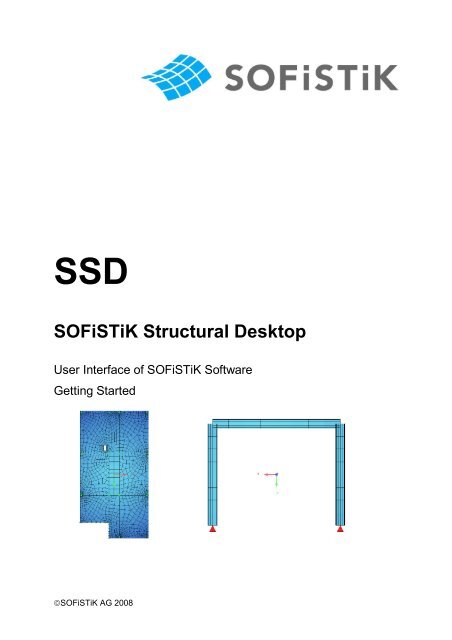
<strong>SSD</strong><br />
<strong>SOFiSTiK</strong> Structural Desktop<br />
User Interface of <strong>SOFiSTiK</strong> Software<br />
Getting Started<br />
©<strong>SOFiSTiK</strong> <strong>AG</strong> 2008
This manual is protected by copyright laws. No part of it may be translated, copied or<br />
reproduced, in any form or by any means, without written permission from <strong>SOFiSTiK</strong> <strong>AG</strong>.<br />
<strong>SOFiSTiK</strong> reserves the right to modify or to release new editions of this manual.<br />
The manual and the program have been thoroughly checked for errors. However, <strong>SOFiSTiK</strong><br />
does not claim that either one is completely error free. Errors and omissions are corrected as<br />
soon as they are detected.<br />
The user of the program is solely responsible for the applications. We strongly encourage the<br />
user to test the correctness of all calculations at least by random sampling.
<strong>SSD</strong> <strong>SOFiSTiK</strong> Structural Desktop<br />
Contents<br />
1 Preface...........................................................................................................................1<br />
2 Basics <strong>SSD</strong>.....................................................................................................................2<br />
2.1 Overview.................................................................................................................2<br />
2.2 User interface <strong>SSD</strong>.................................................................................................3<br />
2.3 Basic Workflow.......................................................................................................4<br />
2.3.1 Groups................................................................................................................4<br />
2.3.2 Tasks..................................................................................................................5<br />
2.3.3 Template files .SOFiSTiX.......................................................................7<br />
2.4 Structure and Function Mode................................................................................10<br />
2.4.1 Computation status...........................................................................................10<br />
2.4.2 <strong>SOFiSTiK</strong> Options.............................................................................................11<br />
2.4.3 Files..................................................................................................................15<br />
3 Basics of SOFiPLUS(-X)...............................................................................................16<br />
3.1 Basic Input............................................................................................................16<br />
3.1.1 Structural Elements...........................................................................................16<br />
3.1.2 Finite Elements.................................................................................................18<br />
4 Example Flat Slab.........................................................................................................19<br />
4.1 Problem................................................................................................................20<br />
4.2 Step 1: Starting <strong>SSD</strong>.............................................................................................21<br />
4.3 Step 2: Materials and Cross Sections...................................................................22<br />
4.4 Step 3: Graphical Input.........................................................................................23<br />
4.5 Step 4: Analysis and Combinations.......................................................................29<br />
4.6 Step 5: Design......................................................................................................33<br />
4.6.1 Design Parameters...........................................................................................33<br />
4.6.2 Design in ULS...................................................................................................36<br />
4.6.3 Design in SLS...................................................................................................38<br />
4.7 Documentation......................................................................................................39<br />
4.8 Discussion of results.............................................................................................40<br />
4.8.1 Structural Analysis............................................................................................40<br />
4.8.2 Punching Design...............................................................................................41<br />
4.8.3 Serviceability.....................................................................................................44<br />
5 Example Steel Design...................................................................................................46<br />
5.1 Problem................................................................................................................46<br />
5.2 Step 1: Input System.............................................................................................47<br />
5.3 Step 2: Cross sections..........................................................................................49<br />
Inhaltsverzeichnis i
<strong>SSD</strong> <strong>SOFiSTiK</strong> Structural Desktop<br />
5.4 Graphic System - and Load Definition...................................................................50<br />
5.4.1 Step 3: Graphic Model Creation........................................................................50<br />
5.4.2 Step 4: Graphic Load Definition........................................................................51<br />
5.4.3 Export to Central Data Base.............................................................................54<br />
5.5 Numeric System- and Load Definition...................................................................55<br />
5.5.1 Step 3: Numeric System Definition....................................................................55<br />
5.5.2 Step 4: Numeric Load Definition........................................................................58<br />
5.6 Step 5: Loadcase Combination Manager..............................................................60<br />
5.7 Step 6: Nonlinear Analysis....................................................................................61<br />
5.8 Step 7: Design Steel Construction........................................................................62<br />
5.9 Appraisal of Results..............................................................................................64<br />
6 <strong>SSD</strong> Functionality..........................................................................................................65<br />
6.1 Description TASKS...............................................................................................65<br />
6.2 Bore Profile...........................................................................................................67<br />
6.3 Work Laws for Springs an Implicit Beam Hinges...................................................69<br />
6.4 Prestressing Systems...........................................................................................69<br />
6.5 Design ULS –Beams.............................................................................................70<br />
6.6 Design ACCI –Beams...........................................................................................71<br />
6.7 Design SLS –Beams.............................................................................................72<br />
6.8 Non-linear Analysis in ULS...................................................................................73<br />
6.9 Non-linear Analysis in SLS...................................................................................74<br />
6.10 Construction Stage Manager................................................................................74<br />
6.11 Eigenvalues..........................................................................................................75<br />
6.12 Buckling Eigenvalues............................................................................................76<br />
6.13 Design RC Section...............................................................................................77<br />
6.14 Summary of Masses.............................................................................................78<br />
7 Support.........................................................................................................................79<br />
8 Literature.......................................................................................................................81
<strong>SSD</strong> <strong>SOFiSTiK</strong> Structural Desktop<br />
1 Preface<br />
Dear <strong>SOFiSTiK</strong> Customer,<br />
With the FEA Version 23 and the <strong>SOFiSTiK</strong> Structural Desktop (<strong>SSD</strong>), you have the latest<br />
development. The <strong>SOFiSTiK</strong> Structural desktop (<strong>SSD</strong>) represents a uniform user interface<br />
for the entire range of <strong>SOFiSTiK</strong>-Software. The <strong>SSD</strong> module controls Pre-processing,<br />
Processing and Post processing.<br />
This <strong>Tutorial</strong> provides you with a short overview and by means of simple examples a fast<br />
entry to the <strong>SSD</strong>.<br />
In the chapter Basic Workflow we introduce the <strong>SSD</strong>’s new user interface and explain the<br />
fundamental functionality of the individual areas.<br />
The following chapters execute several examples with the <strong>SSD</strong>. All essential steps are<br />
described descriptively so they can simply be reproduced by you. We chose standard<br />
examples from literature so that you can compare the results directly.<br />
In the last chapter the essential functions of the <strong>SSD</strong> are arranged and expounded.<br />
We now wish you much success with the execution of the software.<br />
Your <strong>SOFiSTiK</strong> Team<br />
Preface 1
<strong>SSD</strong> <strong>SOFiSTiK</strong> Structural Desktop<br />
2 Basics <strong>SSD</strong><br />
2.1 Overview<br />
In order to understand the operation of the <strong>SOFiSTiK</strong> programs, the basic program structure<br />
is represented subsequently. It is imperative, that all data is stored in a central data base<br />
(<strong>SOFiSTiK</strong> Database CDB).<br />
The <strong>SOFiSTiK</strong> software has a modular structure. The <strong>SOFiSTiK</strong> Structural Desktop (<strong>SSD</strong>)<br />
controls the communication between all of the individual application programs.<br />
Basics <strong>SSD</strong> 2
<strong>SSD</strong> <strong>SOFiSTiK</strong> Structural Desktop<br />
2.2 User interface <strong>SSD</strong><br />
The <strong>SOFiSTiK</strong> Structural Desktop (<strong>SSD</strong>) represents a uniform user interface for the total<br />
range of <strong>SOFiSTiK</strong> software. The module controls pre processing, processing and post<br />
processing. The system can be entered graphically with SOFiPLUS(-X) or as parameterised<br />
text input using TEDDY. The control of the calculation and design process takes place using<br />
dialog boxes, which are accessed via the task tree.<br />
The screen is divided into three main areas.<br />
1. task tree 2. table area 3. work area<br />
Figure 1: Division of <strong>SSD</strong> screen<br />
Basics <strong>SSD</strong> 3
<strong>SSD</strong> <strong>SOFiSTiK</strong> Structural Desktop<br />
2.3 Basic Workflow<br />
The <strong>SSD</strong> is task oriented. The tasks are arranged in groups (e.g. the group "System and<br />
load" contains the tasks materials, cross sections, geometry and loads).<br />
When creating a new project, the necessary groups and tasks are set by default depending<br />
on the chosen problem.<br />
2.3.1 Groups<br />
The computational groups are organized in a tree-structure. This structure can be changed<br />
by the user at any time, as the individual tasks can be dragged to the desired place with the<br />
mouse. The user can remove or insert additional groups at any time with associated tasks.<br />
Figure 2: Group structure <strong>SSD</strong><br />
Example of a possible group-structure of<br />
the <strong>SSD</strong>:<br />
System<br />
- System and load<br />
Linear Analysis<br />
- Calculation and Superposition<br />
Design Area Elements<br />
- Design ULS and SLS<br />
Basics <strong>SSD</strong> 4
<strong>SSD</strong> <strong>SOFiSTiK</strong> Structural Desktop<br />
2.3.2 Tasks<br />
The tasks available are accessed via the right-click-menu in the task tree. They can be<br />
inserted at any place within the tree. When you select the command “insert task” with the<br />
right mouse-button, the following dialog with all available tasks appears.<br />
Figure 3: List of the tasks<br />
Basics <strong>SSD</strong> 5
<strong>SSD</strong> <strong>SOFiSTiK</strong> Structural Desktop<br />
2.3.2.1 Task Tree<br />
In the task tree the options are accessed via the right-click-menu which automatically adjusts<br />
itself to show only those available.<br />
Figure 4: Right click menu in the task tree<br />
2.3.2.2 Table Area<br />
Figure 5: Table area<br />
Right click menu in the task tree<br />
The right click menu will provide<br />
relevant functions for the selected<br />
task.<br />
Examples:<br />
Process Dialog<br />
Edit Text-Input (.DAT)<br />
Reports Result viewer<br />
(name.PLB)<br />
Database information is written in the<br />
table area.<br />
Possible categories:<br />
- Geometry<br />
- Loads<br />
- Results<br />
These results can be copied with right<br />
clicking menu into the clipboard<br />
Possible format:<br />
- Text - Format<br />
- EXCEL- Format<br />
Basics <strong>SSD</strong> 6
<strong>SSD</strong> <strong>SOFiSTiK</strong> Structural Desktop<br />
2.3.2.3 Work Area<br />
The work area displays the ANIMATOR visualisation of the system by default. The work area<br />
changes to WinPS during processing to show calculation status and the TEDDY for further<br />
text input prior to analysis. The graphical input with SOFiPLUS(-X) operates within its own<br />
separate window, making the best possible use of dual monitors.<br />
2.3.3 Template files .SOFiSTiX<br />
For processing of frequently recurrent standard tasks, the Template files of the type<br />
.SOFiSTiX are provided. General Templates are saved in a subdirectory of the<br />
<strong>SOFiSTiK</strong> directory, for example C:\Programs\<strong>SOFiSTiK</strong>\<strong>SOFiSTiK</strong>.23\ <strong>SSD</strong>-Templates.<br />
2.3.3.1 Adding User- defined Template directories<br />
For own Templates, the user can define further Template-directories.<br />
⇒ <strong>SOFiSTiK</strong> Options… <strong>SSD</strong>-Template Path (Find-Button Suchen2.ico ) and Add<br />
In this directory, further subdirectories can be created. These subdirectories appear as tabs<br />
and template icons (see Figure 9). There is only one level of subdirectories available.<br />
Figure 6: <strong>SOFiSTiK</strong> Options <strong>SSD</strong>-Template Path<br />
Basics <strong>SSD</strong> 7
<strong>SSD</strong> <strong>SOFiSTiK</strong> Structural Desktop<br />
2.3.3.2 User Defined Template Files<br />
Any file .<strong>SOFiSTiK</strong> can be stored into the desired Template-Directory as Template<br />
.SOFiSTiX.<br />
All current project settings can be saved as Templates Including the arrangement<br />
and sequence of the tasks. The materials and cross sections are dependent on<br />
the chosen design code. A fixed design code cannot be changed within the<br />
project. File Save As Template<br />
Figure 7: Dialog Save Project as Template<br />
Figure 8: File Save as Template<br />
File New Project from Template<br />
A later changing of the<br />
code is possible if the<br />
Template is stored “without<br />
design code".<br />
The saved file .SOFiSTiX is now available as a further Template.<br />
The existing Template directories<br />
are shown under Directories.<br />
Basics <strong>SSD</strong> 8
<strong>SSD</strong> <strong>SOFiSTiK</strong> Structural Desktop<br />
2.3.3.3 Usage of Template Files .SOFiSTiX<br />
⇒ File New Project from Template…<br />
The existing Templates from the Template path are offered.<br />
Figure 9: File New Project from Template ...<br />
Root directory:<br />
„General“<br />
Subdirectory:<br />
„Concrete“<br />
„Steel“<br />
The desired file .SOFiSTiX is selected and stored under a new data file name with<br />
the button “Save As…” into a project directory.<br />
The new file contains all tasks of the Template. In addition, the data (for example cross-<br />
sections, geometry... etc.) from the Template are transferred into the new file. The data is<br />
then immediately ready for calculation.<br />
With "Templates without Design Code”, the design code can be altered. The<br />
materials and cross sections must be checked and amended.<br />
Basics <strong>SSD</strong> 9
<strong>SSD</strong> <strong>SOFiSTiK</strong> Structural Desktop<br />
2.4 Structure and Function Mode<br />
2.4.1 Computation status<br />
Every task has its own symbol to show the actual computation status<br />
Without computation Input is written directly into the database<br />
Green check mark No computation required<br />
Blue arrow New input data computation required<br />
Blue cross Old data computation required<br />
Red cross Error message computation required<br />
Green cross Warning message computation required (possibly)<br />
Figure 10: Computation status<br />
Basics <strong>SSD</strong> 10
<strong>SSD</strong> <strong>SOFiSTiK</strong> Structural Desktop<br />
2.4.2 <strong>SOFiSTiK</strong> Options<br />
Numerous settings within the options dialog are possible of which only the most important<br />
are introduced now.<br />
2.4.2.1 Language Settings<br />
There is a difference between the dialog box language and the input/output language. The<br />
dialog box language is stored within the REGISTRY of the local computer. The <strong>SSD</strong> must be<br />
started again so that this alteration is activated. The input/output language is stored within<br />
the file <strong>SOFiSTiK</strong>.DEF.<br />
Figure 11: Dialog <strong>SOFiSTiK</strong>: Options Language<br />
2.4.2.2 Project defaults<br />
With the option Project Defaults, the user can assign default attributes of new projects. In<br />
addition, the user can define if graphical or text is the default input. These attitudes are<br />
stored in the Registry.<br />
Basics <strong>SSD</strong> 11
<strong>SSD</strong> <strong>SOFiSTiK</strong> Structural Desktop<br />
Figure 12: Dialog <strong>SOFiSTiK</strong>: Options Project defaults<br />
Basics <strong>SSD</strong> 12
<strong>SSD</strong> <strong>SOFiSTiK</strong> Structural Desktop<br />
2.4.2.3 Process the environment variables in the file <strong>SOFiSTiK</strong>.DEF<br />
The <strong>SOFiSTiK</strong> dialog supports numerous parameters, which are defined as environment<br />
variables (in the Environment, in the <strong>SOFiSTiK</strong>.DEF or in the local .DAT). General<br />
defaults are preferably stored in the file <strong>SOFiSTiK</strong>.DEF. In the following example, the input of<br />
a modified company heading takes place in the results listing with the variable<br />
<strong>SOFiSTiK</strong>_NAME.<br />
⇒ <strong>SOFiSTiK</strong> Options Edit File “sofistik.def“ Select <strong>SOFiSTiK</strong>-DEF file with<br />
a tick Edit Button<br />
Figure 13: Dialog <strong>SOFiSTiK</strong>: Options Edit <strong>SOFiSTiK</strong>.DEF<br />
Basics <strong>SSD</strong> 13
<strong>SSD</strong> <strong>SOFiSTiK</strong> Structural Desktop<br />
The pre-defined parameters are displayed with the button “New”.<br />
Figure 14: Dialog: Pre-defined parameters<br />
Figure 15: Allocation of an environment variable<br />
The modified company name now is<br />
assigned to the key of<br />
<strong>SOFiSTiK</strong>_NAME as value:<br />
"Jack Miller"<br />
Pressing OK stores the new values.<br />
However, the program must be closed<br />
and re-launched for the new settings to<br />
apply.<br />
The principle hierarchy of the definition files <strong>SOFiSTiK</strong>.DEF is shown in Figure 13. The<br />
different files <strong>SOFiSTiK</strong>.DEF are checked in succession one after the other. Highest priority<br />
has the setting, which is stored in the <strong>SOFiSTiK</strong>.DEF file in the project directory. The path of<br />
the <strong>SOFiSTiK</strong> variable is checked off afterwards. If no <strong>SOFiSTiK</strong> variable is defined in the<br />
Environment, the <strong>SOFiSTiK</strong> directory is used as default.<br />
Basics <strong>SSD</strong> 14
<strong>SSD</strong> <strong>SOFiSTiK</strong> Structural Desktop<br />
2.4.3 Files<br />
The basic files are arranged in the following table:<br />
Name.<strong>SOFiSTiK</strong> Central XLM- file where all information is saved.<br />
Name.DAT Control file, ASCII format<br />
Name.PLB For each task the result is saved in a file task.PLB. This file can be<br />
Name.CDB Central data base<br />
shown and/or printed out individually. Also it can be assigned to<br />
the total result using the command "all results".<br />
Name.DWG Using graphical input all information about system and loading is<br />
saved in this drawing.<br />
Name.SOFiSTiX Template- file in XLM- format: File in Template- directory.<br />
Table 1: Overview of the file- Extensions<br />
Basics <strong>SSD</strong> 15
<strong>SSD</strong> <strong>SOFiSTiK</strong> Structural Desktop<br />
3 Basics of SOFiPLUS(-X)<br />
3.1 Basic Input<br />
SOFiPLUS(-X) is a graphic user interface (GUI) for the system generation based on<br />
AutoCAD and ADT.<br />
There are two basic generation principles. First you may generate the systems by directly<br />
defining the finite elements. Every element and node has to be drawn separately and the<br />
system will be generated out of this input. Second you may define the system by structural<br />
elements, which are only the wire frame of the structure. After that an automatic mesh<br />
generation will create the finite element system for further analysis.<br />
The important differences are described below. For further information please<br />
see the SOFiPLUS(-X) HELP file.<br />
3.1.1 Structural Elements<br />
The definition of Finite Elements starts with the toolbox “SOFiPLUS Classic Create<br />
Structure”. Structural Areas, Structural Lines and Structural Points are the main elements for<br />
the structure definition.<br />
The basic functionality of Structural Elements are:<br />
- Structural Area<br />
- Curved Area<br />
- Opening<br />
- Structural Line<br />
- Structural Point<br />
- DWG SOFIMSHB<br />
- The meshing is done externally<br />
- No FE-mesh!<br />
- Copying elements including object attributes is possible<br />
The basic idea with the structural elements is to create a wire frame of the structure. For this<br />
all AutoCAD commands can be used. After finishing the wire frame model the automatic<br />
Basics of SOFiPLUS(-X) 16
<strong>SSD</strong> <strong>SOFiSTiK</strong> Structural Desktop<br />
mesh generation will create a finite element system and an input data file .DAT<br />
which can be modified using TEDDY.<br />
Important is the possibility to define “Free Nodes”, which are independent from mesh and<br />
structure. You also may define loads connected to structural elements.<br />
The analysis will be started directly out of SOFiPLUS or with WinPS.<br />
A mixture of Finite Elements and Structural Elements is possible under special conditions.<br />
We recommend avoiding any mixture if at all possible.<br />
The Post processing can be done with the normal programs like WinGRAF, DBPRIN and<br />
DBView. For the documentation use the URSULA result browser.<br />
The most important attributes are:<br />
Structure Area<br />
- Defined by Structure Points and Structure Lines<br />
- Plane and curved areas are available<br />
- = geometric area in SOFiMSHB (GAR)<br />
Structural Line<br />
- Area boundary<br />
- Defined by ≥2 Structure Points<br />
- Geometric restraint for SOFiMSHB<br />
- Definition of linear support conditions<br />
- Definition of linear coupling<br />
- Beam, Truss or Cable element<br />
- Pile Element<br />
- Form: straight line, arch, spline<br />
- = geometric line in SOFiMSHB (GLN)<br />
Structure Point<br />
- Geometric restraint for SOFiMSHB<br />
- Part of Structure Line<br />
- Single Support condition<br />
- Column including dimensions for punching design<br />
- Spring<br />
- = geometric point in SOFiMSHB (GPT)<br />
Basics of SOFiPLUS(-X) 17
<strong>SSD</strong> <strong>SOFiSTiK</strong> Structural Desktop<br />
3.1.2 Finite Elements<br />
The definition of Finite Elements starts with the toolbox “SOFiPLUS-Classic Create<br />
Elements”. Nodes, constraints, beams, springs, truss elements, cables, boundary elements<br />
and area elements are possible elements.<br />
The basic functionality of Finite Elements are:<br />
- FE Elements are produced directly in AutoCAD<br />
- Meshing is done directly in AutoCAD<br />
- CDB export / import<br />
- Copying of elements is possible<br />
Macros available for different mesh generation<br />
Basics of SOFiPLUS(-X) 18
<strong>SSD</strong> <strong>SOFiSTiK</strong> Structural Desktop<br />
4 Example Flat Slab<br />
Example is taken from reference [1], and [2]<br />
Figure 16: Geometry of Slab<br />
Example Flat Slab 19
<strong>SSD</strong> <strong>SOFiSTiK</strong> Structural Desktop<br />
4.1 Problem<br />
A concrete and punching design according to German code DIN 1045-1 for the slab shown in<br />
Figure 16 is required.<br />
Materials: concrete C 30/37<br />
reinforcement BST 500<br />
Exposition class XC1, concrete cover cnom = 20 mm<br />
Columns: Ø 45 cm floor height 3,0 m<br />
Walls: d = 30 cm floor height 3,0 m<br />
Slab: d = 24 cm<br />
Loads:<br />
Dead loads (G)<br />
Self weight slab 0,24 · 25 = 6,00 kN/m² (automatic calculation)<br />
Dead load 1,50 + 0,50 = 2,00 kN/m²<br />
Variable loads (Q)<br />
Live load = 5,00 kN/m²<br />
The following structural design calculations will be done:<br />
Ultimate limit state (ULS)<br />
Serviceability limit state (SLS)<br />
Punching design<br />
Non linear analysis with cracked concrete for long term displacements<br />
The following example shows the basic workflow right from the beginning of a project with<br />
the definition of geometry and loads, then analysis and design with the final documentation of<br />
results.<br />
Example Flat Slab 20
<strong>SSD</strong> <strong>SOFiSTiK</strong> Structural Desktop<br />
4.2 Step 1: Starting <strong>SSD</strong><br />
First of all we have to start the <strong>SSD</strong> with a double click on the button , which should be<br />
located on your desktop. To open a new project please use the button / or go via the top<br />
menu using: File > New Project…<br />
After that the following dialog will open. Please add title, database name and directory.<br />
Also select design code, system, calculation and choose the option “Graphical Pre-<br />
processing”.<br />
Figure 17: Start dialog – System Information<br />
With selection of “Graphical Pre-processing” additional input is necessary. The default<br />
settings are usually OK. Important is the input of the system size. Confirming the input with<br />
OK, the program starts a central database exp1-flatslab.cdb.<br />
Example Flat Slab 21
<strong>SSD</strong> <strong>SOFiSTiK</strong> Structural Desktop<br />
Changing the design code after saving the project is not possible.<br />
Figure 18: Main window <strong>SSD</strong> -<br />
As described in chapter 2.3.2.1 the task tree is placed on the left side. With this tree you can<br />
access all groups and tasks within the project.<br />
The next step is to define materials and cross sections.<br />
4.3 Step 2: Materials and Cross Sections<br />
Four default materials concrete C 20/25, reinforcement BSt 500, steel S 235 and brick MZ4 I<br />
Figure 19: Dialog Material<br />
are created. To modify the materials<br />
open the dialog with a double click.<br />
The material number 1 concrete C<br />
20/25 has to be changed to a concrete<br />
30/37. Change the classification from<br />
20 to 30. Confirm the change with the<br />
OK button.<br />
To delete a material simply use the<br />
right mouse click DELETE.<br />
Example Flat Slab 22
<strong>SSD</strong> <strong>SOFiSTiK</strong> Structural Desktop<br />
4.4 Step 3: Graphical Input<br />
For system and load generation the graphical input the program SOFiPLUS(-X) will be used.<br />
Now double click on the task “GUI for Model Creation (SOFiPLUS(-X))“ to open it.<br />
_line<br />
SOF_PM_STEDGE<br />
SOF_PM_STPOINT<br />
First of all start the drawing of the outline of the slab by using the<br />
AutoCAD command ‘line’.. The coordinate origin is located at the top<br />
left corner of the slab. Start drawing the outline from the point (0,0) and<br />
continue with the following dimensions and directions. .<br />
11,850 horizontal to the right ",<br />
22.050 vertical down $,<br />
6.825 horizontal to the left!,<br />
2.725 vertical up#,<br />
5.025 horizontal to the left !,<br />
19.325 vertical up#,<br />
Finish the command with ESC<br />
Create structural lines from this outline by opening the command<br />
“Structural Line” and select the option “select entity” from the right click<br />
menu. Use a selection rectangle starting at the bottom right and moving<br />
to the top left side. Confirm the selection by pressing Return.<br />
Now start the definition of the columns using the command “Structure<br />
Point”. The structure points we are going to define now are also the<br />
column supports and will be used for punching checks.<br />
Example Flat Slab 23
<strong>SSD</strong> <strong>SOFiSTiK</strong> Structural Desktop<br />
Every column has a diameter of 45 cm. For the support conditions select<br />
the tab ‘bottom columns’ and apply both the rotational and vertical<br />
springs. The spring stiffness is calculated automatically from the cross<br />
section, the floor height and the material information provided. The<br />
rotational spring stiffness has to be changed to 257000 kNm/rad as<br />
written in reference [1] and [2].<br />
The columns are simple to create by using the cursor in the drawing<br />
screen. For each column the following coordinates have to be used.<br />
(0.225/0.225) (5.025/0.225) (6.825/0.225) (11.625/0.225)<br />
(0.225/7.425) (5.025/7.425) (6.825/7.425) (11.625/7.425)<br />
(0.225/14.625) (5.025/14.625) (6.825/14.625) (11.625/14.625)<br />
(6.825/21.825) (11.625/21.825)<br />
We recommend defining every load area as a structural area. The program<br />
automatically creates loadcases for every area.<br />
SOF_PM_STEDGE<br />
SOF_PM_STAREA<br />
To define structural areas easily, additional structural lines are<br />
necessary. Therefore, create new structural lines between the columns<br />
and between column and slab outline until the slab is partitioned as<br />
shown in Figure 20.<br />
After defining the additional structural lines the structural areas can then<br />
be defined. The slab thickness is 0.24 m.<br />
There are four methods to define a structure area. The simplest way is<br />
to click into the drawing screen. Please use “select point in area” from<br />
the right click menu and click inside the first area.<br />
Example Flat Slab 24
<strong>SSD</strong> <strong>SOFiSTiK</strong> Structural Desktop<br />
For load definition open the dialog<br />
“Loads on Slabs” and add 2.0 kN/m² for<br />
the dead load (LC 1) and 5.0 kN/m² for<br />
the following live loads (LC 2, 3 …).<br />
Confirm the input with OK.<br />
The loadcase number of the live loads will increase by 1 automatically.<br />
Opening<br />
SOF_PM_EDGE_M<br />
Please add an opening. First we recommend drawing the opening<br />
outline using normal AutoCAD Lines. Then start the command<br />
“Opening” and chose “PICK point within opening” After clicking inside<br />
the opening the definition is finished.<br />
Finally the wall supports (A’/1-2 and 2/a-A’) have to be defined. Select<br />
the command “structural line” and modify the wall as shown below. The<br />
support width of 0.3 m is important for the following punching design.<br />
We recommend using nonlinear supports with a wall stiffness calculated<br />
from the wall thickness 0.30 m and the floor height 3.0 m. Use the<br />
button “Wall stiffness …”. Confirm the input with OK.<br />
Example Flat Slab 25
<strong>SSD</strong> <strong>SOFiSTiK</strong> Structural Desktop<br />
Now the graphical input is finished, see Figure 20.<br />
Figure 20: Complete slab system<br />
Example Flat Slab 26
<strong>SSD</strong> <strong>SOFiSTiK</strong> Structural Desktop<br />
Before starting the automatic mesh generation we recommend checking the actions and<br />
loads.<br />
To start the loadcase manager use the button . After the dialog is open you will see the<br />
tab loadcases. There are 10 loadcases listed in the table. The 1 st loadcase is the dead load.<br />
The program is able to calculate automatically the self weight of the construction. To do so<br />
the factor in the row SW has to be changed to 1.0 for LC 1.<br />
Change now to the tab actions. There are two actions defined, total dead load and variable<br />
load., which is correct for this problem. Beside the action name the correct safety and<br />
combination values according to German code DIN 1045-1 are listed.<br />
SOF_glfmod<br />
Click on the button to start the loadcase manager<br />
Listing of loadcases<br />
Listing of actions<br />
Example Flat Slab 27
<strong>SSD</strong> <strong>SOFiSTiK</strong> Structural Desktop<br />
After these checks the system definition is finished and a system export into the central<br />
database is necessary. This will be done by the command button .<br />
Now save your drawing and change back to the main <strong>SSD</strong> window, where the system will be<br />
shown in the ANIMATOR.<br />
Figure 21: ANIMATOR showing complete slab system<br />
The next step is to do the linear analysis for every single loadcase and calculate the relevant<br />
combinations.<br />
SOFiPLUS is able to import any drawing with DWG or DXF format. Therefore<br />
architectural drawings can be used for the system generation<br />
Example Flat Slab 28
<strong>SSD</strong> <strong>SOFiSTiK</strong> Structural Desktop<br />
4.5 Step 4: Analysis and Combinations<br />
To start the linear analysis, open this task with a double click. By default all existing<br />
loadcases are selected. Normally there is no need for a manual selection.<br />
Figure 22: Dialog Linear Analysis – Loadcases Tab<br />
By default all loadcases are selected, which is normally sufficient.<br />
Figure 23: Dialog Linear Analysis – Groups Tab<br />
Example Flat Slab 29
<strong>SSD</strong> <strong>SOFiSTiK</strong> Structural Desktop<br />
Group selection is important. By default all groups will be selected for a calculation.<br />
Deselected groups are not considered during the calculation. This facility can be used to<br />
simulate temporary support conditions during construction. The first loadcases are calculated<br />
with the temporary supports. In the last loadcase, deselect the group containing the<br />
temporary supports for them to be ignored.<br />
In the case where groups of elements are active and passive for different loadcases<br />
it is necessary to define multiple “Linear Analysis” tasks.<br />
It is very important to check the loads because loads on deselected elements will<br />
cause an error message during the calculation.<br />
Control Parameters are not necessary. The register “Text Output” is responsible for the<br />
output and documentation. The output volume is variable for the different output chapters.<br />
Also the default output is sufficient in most cases.<br />
Figure 24: Dialog Linear Analysis – Text Output Tab<br />
Besides the text output a graphical output is also available. There are default settings for<br />
standard graphics. To add these graphics to the output just select or deselect the entries<br />
from the tree structure.<br />
Example Flat Slab 30
<strong>SSD</strong> <strong>SOFiSTiK</strong> Structural Desktop<br />
Figure 25: Dialog Linear Analysis – Graphical Output Tab<br />
Important to note is the ease with which a user defined view can be created. Select the view<br />
option “User defined” and click into the view window and move the system inside the 3D-<br />
orbit.<br />
The import of additional graphic files created with WINGRAF is also possible. Select the<br />
option “Use additional graphics” and start browsing . The other way is to start WINGRAF<br />
with the button. The graphics you define inside WINGRAF will be transferred to the <strong>SSD</strong>.<br />
Confirm all settings with the OK button.<br />
In the bottom left-hand corner you will find the preselected option “Calculate<br />
immediately”. Confirming with OK button will automatically start the calculation.<br />
With the ‘Calculate immediately’ selected,a new program is opened within the <strong>SSD</strong> main<br />
window. On the left-hand side, there is a tree structure, which shows all tasks. Only the two<br />
program blocks SEPP and WING are active for this calculation, which is shown by the signs<br />
.<br />
Example Flat Slab 31
<strong>SSD</strong> <strong>SOFiSTiK</strong> Structural Desktop<br />
Figure 26: <strong>SSD</strong> main window - calculation overview<br />
To change the programs use the task bar at the bottom.<br />
Figure 27: <strong>SSD</strong> main window - ANIMATOR view of LC 1<br />
These basic proceedings will be done now for the Superpositioning<br />
Example Flat Slab 32
<strong>SSD</strong> <strong>SOFiSTiK</strong> Structural Desktop<br />
The task “Select Superpositioning” is a selection only. To create new<br />
superpositions a new task “Define Superpositioning” has to be added.<br />
Always use the task “Select Superpositioning” after the task “Define<br />
Superpositioning” to make sure all superpositions are available and can be<br />
processed by the program.<br />
Figure 28: Dialog Select Superpositioning – Superpositions Tab<br />
The text and graphical output can be selected as shown before. In addition, the option<br />
“Calculate immediately” works in the same way.<br />
4.6 Step 5: Design<br />
By default three design tasks according to the design code were generated automatically.<br />
The tasks are – Design parameters – Design in ULS – Design in SLS -<br />
4.6.1 Design Parameters<br />
The design parameters allow the user to define specific reinforcement for every group of<br />
elements. There are four different reinforcement types available: two layers – orthogonal, two<br />
layers – non orthogonal, three layers and circular.<br />
Example Flat Slab 33
<strong>SSD</strong> <strong>SOFiSTiK</strong> Structural Desktop<br />
Figure 29: Dialog Design Parameters – Register Common<br />
In most cases, two-layer orthogonal reinforcement is suitable for the design. In this dialog,<br />
the main direction and the distances between centreline of reinforcement bars and concrete<br />
surfaces can be edited. If reinforcement has to be changed for selected groups, create a<br />
new line in the Design parameter list using the button NEW.<br />
Then select the relevant groups from the selection list. For example, select groups 1 to 3 and<br />
define a two layer non orthogonal reinforcement with an angle of 45°. The settings for the<br />
other groups will remain the same as shown in Figure 30.<br />
Example Flat Slab 34
<strong>SSD</strong> <strong>SOFiSTiK</strong> Structural Desktop<br />
Figure 30: Dialog Design Parameters – Direction Tab<br />
This example is only to show the input procedure and will not be used in the<br />
following calculation. Therefore please delete this input with the button DELETE.<br />
The other parameters are basically used by the serviceability design.<br />
Diameter Tab: is used for crack width calculation<br />
Minimum Tab: predefined minimum reinforcement for non-linear analysis<br />
Maximum Tab: predefined maximum reinforcement for non-linear analysis<br />
Crack Width Tab: crack width input to determine reinforcement stresses<br />
The definitions made here will be used in all following design tasks.<br />
Example Flat Slab 35
<strong>SSD</strong> <strong>SOFiSTiK</strong> Structural Desktop<br />
4.6.2 Design in ULS<br />
The design in ultimate limit state (ULS) is controlled it’s own task. Generally, (and for the<br />
example) no further input is necessary.<br />
For information, the following input procedures are described as follows.<br />
Figure 31: Dialog Design in ULS – General Tab<br />
The superposition results are loadcases with different identifiers. As shown in Figure 31 there<br />
are the single loadcases (LC 1 – LC 10) and loadcases 21xx from the ultimate design<br />
combination. The program automatically selects all the loadcases for results from the<br />
ultimate design combination. The column Am indicates loadcases with results for area<br />
elements, the column Aa indicates loadcases with additional results for area elements and<br />
the column Be indicates loadcases with results for beam elements. In this example, we don’t<br />
have any beam elements, so the column is clear, which is correct.<br />
For the shear and punching design go to the “Shear Reinforcement” tab. The program will<br />
increase automatically the bending reinforcement to pass the shear and punching checks.<br />
You may define a maximum percentage as an upper limitation for the bending reinforcement<br />
before shear links are required. There is a control over the shear reinforcement design both<br />
Example Flat Slab 36
<strong>SSD</strong> <strong>SOFiSTiK</strong> Structural Desktop<br />
inside and outside the punching area. No increase of reinforcement is allowed in this<br />
example.<br />
Figure 32: Dialog Design in ULS – Shear Reinforcement Tab<br />
Activate the punching checks<br />
and limit the increase of bending<br />
reinforcement with the input of 0.<br />
No increase of bending<br />
reinforcement for shear checks<br />
outside the punching area<br />
Using the Beams tab you may define the necessary design settings for beam elements. If<br />
there are no beams in the system, as in this example, no input is required.<br />
There are various control parameters which can be set depending on the design codes. For<br />
further information we refer you to the national codes and the technical literature.<br />
As with all other tasks, the text and graphical output can be selected.<br />
The calculation starts immediately if the ‘Calculate immediately’ check box is ticked. Please<br />
deactivate the option “Calculate immediately” and after checking all input, close the input with<br />
OK. Now you will see the sign in the task tree. This means, that the task has a new input<br />
and is still open for calculation. (see also Figure 10)<br />
Before starting the calculation you may wish to check the CADINP input data, created<br />
automatically.<br />
Every task automatically creates a CADINP input file, which is part of the complete<br />
input file .dat. To check this input file use the text editor TEDDY. To open<br />
the input file click on the task inside the task tree and use the right mouse click<br />
– EDIT. Now the TEDDY will be opened.<br />
Example Flat Slab 37
<strong>SSD</strong> <strong>SOFiSTiK</strong> Structural Desktop<br />
The TEDDY input file is shown below.<br />
$ Automatically generated by DesignULS V(1.00-23) 15.02.2006 12:39:08<br />
$ Attention: Changes will be overwritten if the task is opened again!<br />
+PROG BEMESS urs:11.1 $ Design in ULS<br />
HEAD ULS design<br />
CTRL LCR 1 $ Reinforcement distribution number<br />
CTRL RO_V 0 $ Maximum reinforcement for shear for normal slab region<br />
PUNC YES RO_V 0<br />
LC DESI<br />
END<br />
The functionality available within TEDDY is very powerful and all can be access within the<br />
<strong>SSD</strong>. Additional text input can be entered to amend or extend that which has been created<br />
with the dialog input. There are numerous possibilities, which are not discussed here. For<br />
further information please look in the handbook <strong>SOFiSTiK</strong>_1.pdf.<br />
Before going on with the “Design in SLS” the calculation “Design in ULS” has to be<br />
finished because reinforcement areas are necessary for SLS input.<br />
Also note, that changes within the dialogs will change the CADINP input file.<br />
4.6.3 Design in SLS<br />
According to the German code DIN 1045-1 the design in Serviceability Limit State is more<br />
important today. The task “Design in SLS” starts a design for the maximum crack width.<br />
Again the relevant loadcases are selected automatically for the design. A manual selection is<br />
not normally necessary.<br />
Figure 33: Dialog Design in SLS – Quad Elements Tab<br />
Crack width is calculated either<br />
due to tabulated values or due<br />
to user defined input.<br />
Normally the design is<br />
done by DIN 1045-1 Table 20.<br />
In case there are some limiting<br />
stresses added in the task<br />
“Design Parameters” the design<br />
will be done by Table 21. In<br />
case bar diameters and stresses<br />
are defined the design follows<br />
again Table 21.<br />
Example Flat Slab 38
<strong>SSD</strong> <strong>SOFiSTiK</strong> Structural Desktop<br />
4.7 Documentation<br />
The documentation is divided into several URSULA reports. After every calculation a task<br />
creates it’s own URSULA report. For the final documentation go to the button and select<br />
“all reports”. URSULA will open automatically and displays the complete report.<br />
Figure 34: URSULA Result browser<br />
All chapters are printed in a tree structure on the left-hand side of the URSULA screen.<br />
Normally every chapter is activated except the “Control of input” chapters. To activate or<br />
deactivate every chapter just click on the chapter title within the tree.<br />
There is an easy way to add a complete list of contents, by using the top menu Insert – Insert<br />
List of Contents.<br />
Example Flat Slab 39
<strong>SSD</strong> <strong>SOFiSTiK</strong> Structural Desktop<br />
4.8 Discussion of results<br />
4.8.1 Structural Analysis<br />
A complete validation of all internal forces is not discussed here. The object here is to<br />
compare the relevant support forces and moments for the following punching check.<br />
Figure 35: Support forces and moments at node 12 LC 1 and LC 2156<br />
Betonkalender 2006, page 183, Figure 101 <strong>SOFiSTiK</strong> <strong>SSD</strong><br />
node12 (S1) dead load live load Max Pzed 1) LC 1: G Max Pzed<br />
Rz [kN] 213 149 511,05 -211,6 -498,1<br />
Mx [kNm] -7,6 -1,15 -11,99 7,28 11,8<br />
My [kNm] 28,8 16,9 64,23 -27,0 -63,0<br />
1) Pzed = 1,35 G +1,50 Q<br />
Table 1: Overview results from literature and out of <strong>SSD</strong> calculation<br />
As shown in Table 1 the results compare very closely with the reference example. The only<br />
difference is the signs, which is caused by the different coordinate systems used in literature<br />
and <strong>SOFiSTiK</strong> <strong>SSD</strong>.<br />
Example Flat Slab 40
<strong>SSD</strong> <strong>SOFiSTiK</strong> Structural Desktop<br />
4.8.2 Punching Design<br />
To check the results we recommend using the extended text output for punching design. The<br />
output volume can be changed in task “Design in ULS” – Text output tab.<br />
For detailed comparison between the results from the reference literature and from the<br />
<strong>SOFiSTiK</strong> calculation we want to look at the punching checks of node 3 (wall corner) and<br />
node 12 (inner column near hole). The detailed text output is printed below:-<br />
Punching Design (DIN1045-1)<br />
Node number = 3 X= 5.025 [m] Y= 19.33 [m]<br />
Max. shear force V-ULS= 246.8 [kN] LC= 2102 via QUAD connecting forces<br />
Integrated from boundary reactions over a length of 2*0.294 [m]<br />
Wall corner a= 0.294 [m]<br />
The active wall length a has been set to 1.4*depth. Wall thickness is not used.<br />
Plate thickness h-slab= 0.240 [m] depth 0.210 [m]<br />
1. perimeter at 1.5*d= 0.315 [m] ucrit= 1.227 [m]<br />
(u= 39 % of utot due to openings, edges or walls)<br />
Tension reinfor. as >= 14.89 [cm2/m] mue= 0.71 [o/o] VRdct 160.9 [kN/m]<br />
mue necessary to satisfy von vRD,max acc. DIN 1045-1 equation 107!<br />
v-Ed = 1.20*V/ucrit = 241.4 [kN/m] > 160.9 [kN/m] =Vrdct<br />
1.20=sweeping excentricityfaktor beta<br />
Beta value end of walls/corners acc. Normenausschuß Bau [NABAU] Lfd 233 10.5.2<br />
1. design cut of shear reinforcement at point 0.5d -> u= 0.714 [m]<br />
Shear reinforcem. Ass= (V-Ed*ucrit/u-VRdc)*u/fyd/kappa-s (kappa-s=0.70)<br />
Shear reinforcem. Ass= 5.96 [cm2] ass= 52.99 [cm2/m2]<br />
to be provided in the 1. perimeter up to columnedge + 0.184 [m]<br />
2. perimeter Ass= 2.94 [cm2] ass= 17.00 [cm2/m2] til 0.341 [m]<br />
Ass= (V-Ed(u)-VRdc)*u*sw/d/fyd/kappa-s<br />
3. perimeter Ass= 1.42 [cm2] ass= 6.06 [cm2/m2] til 0.499 [m]<br />
In the critical punching zone at least 14.89 [cm2/m]<br />
tension reinforcement is required<br />
.<br />
Node number = 12 X= 5.025 [m] Y= 7.425 [m]<br />
Max. shear force V-ULS= 517.8 [kN] LC= 2104 via QUAD connecting forces<br />
Circular column dS= 0.450 [m]<br />
Plate thickness h-slab= 0.240 [m] depth 0.210 [m]<br />
1. perimeter at 1.5*d= 0.315 [m] utot= 3.393 [m] ucrit= 3.016 [m]<br />
(u= 89 % of utot due to openings, edges or walls-> edge column)<br />
Min.reinforc. as-upper= 16.08 [cm2/m] (Min.design-moment-> edge column)<br />
Min.reinforc as-lower= 7.52 [cm2/m] (Min.design-moment-> edge column)<br />
Tension reinfor. as >= 16.08 [cm2/m] mue= 0.77 [o/o] VRdct 165.1 [kN/m]<br />
mue necessary to satisfy von vRD,max acc. DIN 1045-1 equation 107!<br />
v-Ed = 1.20*V/ucrit = 206.0 [kN/m] > 165.1 [kN/m] =Vrdct<br />
1.20=sweeping excentricityfaktor beta<br />
1. design cut of shear reinforcement at point 0.5d -> u= 1.843 [m]<br />
Shear reinforcem. Ass= (V-Ed*ucrit/u-VRdc)*u/fyd/kappa-s (kappa-s=0.70)<br />
Shear reinforcem. Ass= 10.41 [cm2] ass= 35.87 [cm2/m2]<br />
to be provided in the 1. perimeter up to columnedge + 0.184 [m]<br />
2. perimeter Ass= 4.23 [cm2] ass= 9.86 [cm2/m2] til 0.341 [m]<br />
Ass= (V-Ed(u)-VRdc)*u*sw/d/fyd/kappa-s<br />
In the critical punching zone at least 16.08 [cm2/m]<br />
tension reinforcement is required<br />
In addition to the extended output a short table “Conclusions” is also printed in the output.<br />
Important are the additional hints written below this listing. As you can see, the Column at<br />
node 12 will be treated as an edge column because of the adjacent opening Therefore, node<br />
12 is marked with Typ E = edge column.<br />
Example Flat Slab 41
<strong>SSD</strong> <strong>SOFiSTiK</strong> Structural Desktop<br />
Punching Design (DIN1045-1)<br />
CONCLUSION<br />
NodeNo Typ X Y V-ULS d-col ucrit =%u0 v-max AssSum ast nperi<br />
No [m] [m] [kN] [m] [m] [o/o] [MPa] [cm2] [cm2/m]<br />
3 L 5.025 19.325 246.8 0.332 1.227 39 1.15 10.32 14.89 3<br />
12 E 5.025 7.425 517.8 0.450 3.016 89 0.98 14.64 16.08 2<br />
Typ I=inner column, E=edge column, C=corner column, F=foundation,<br />
W=end of wall, L=wall corner, G=end_of_girder<br />
ucrit =effective length of 1. perimeter, reduced due to openings and edges<br />
%u0 =reduktionfactor due to openings and free edges = u0/u0-tot in %<br />
AssSum=shear reinforcement - total sum of all nperi perimeters<br />
ast = min. required tension reinforcement in the punching zone<br />
nperi =up to this perimeter, shear reinforcement is required<br />
Both pressure and tension results are taken into account.<br />
Minimim design moments and collapse reinforcement are taken into account.<br />
4.8.2.1 Punching inner column, node 12<br />
Literature <strong>SOFiSTiK</strong><br />
Effective height [cm] 20 21<br />
Diameter critical perimeter dkrit [m] 1,05 1,08<br />
Reduction due to opening δ [-] 0,8819 0,89<br />
Critical perimeter ukrit [m] 2,91 3,016<br />
factor β 1,29 1,20<br />
Shear force ved [kN/m] 227 206,0<br />
shear capacity without reinforcement vRd,ct [kN/m] 190,0 165,1<br />
Shear reinforcement 1. perimeter [cm²]<br />
distance 0,5d=10,5 cm up to 0,5d+sw/2=18,4 cm<br />
10,40 10.41<br />
Design cut u1 [m] 1,80 1,843<br />
Shear reinforcement 2. perimeter [cm²]<br />
distance 18,4 cm up to<br />
0,5d + 3 • sw/2 = 10,5+ 3 • 15,75 /2 = 34,1 cm<br />
3,95 4,23<br />
Design cut u2 [m] 2,63 2,72<br />
Table 2: Comparison of results from literature and from <strong>SOFiSTiK</strong> calculation at node 12<br />
The results compare very well. The slight difference is caused by different effective heights,<br />
different bending reinforcement and different factor β which takes into account the opening.<br />
Reducing the critical perimeter near inner columns by up to 80%, the factor β is<br />
considered with 1,20 instead of 1,05 (DIN 1045-1, Figure 44). The column will be<br />
treated as type E = edge column.<br />
Example Flat Slab 42
<strong>SSD</strong> <strong>SOFiSTiK</strong> Structural Desktop<br />
4.8.2.2 Punching check at wall corner, node 3<br />
The punching design on wall corners must be treated in a special way.<br />
Figure 36: WINGRAF Figure- punching check at node 3<br />
For further description we refer to our BEMESS manual Chapter 2.4.6.<br />
Example Flat Slab 43
<strong>SSD</strong> <strong>SOFiSTiK</strong> Structural Desktop<br />
4.8.3 Serviceability<br />
The results of the serviceability check are also printed in the URSULA output. The output is<br />
organized in several chapters. The reinforcement from the ultimate limit state design is saved<br />
in a reinforcement loadcase, which will be used now. Next is a list of loadcases which will be<br />
used for the design.<br />
Maximum of reinforcement-distributions<br />
The reinforcement maximum was build out of the numbers of reinforcementdistributions:<br />
1<br />
and stored as new reinforcement-distribution 2 .<br />
Design according to DIN1045-1<br />
Loadcases have been calculated in the Serviceability State<br />
In BEMESS no additional load safety factor is applied.<br />
Load Cases for the Design<br />
Loadcase 1701 MAXP-MXX Forces and mome<br />
Loadcase 1702 MINP-MXX Forces and mome<br />
Loadcase 1703 MAXP-MYY Forces and mome<br />
Loadcase 1704 MINP-MYY Forces and mome<br />
Loadcase 1705 MAXP-MXY Forces and mome<br />
Loadcase 1706 MINP-MXY Forces and mome<br />
Loadcase 1707 MAXP-VX Forces and mome<br />
Loadcase 1708 MINP-VX Forces and mome<br />
Loadcase 1709 MAXP-VY Forces and mome<br />
Loadcase 1710 MINP-VY Forces and mome<br />
Loadcase 1717 MAXP-P Bedding stresse Bedding stresses for punching design<br />
Loadcase 1718 MINP-P Bedding stresse Bedding stresses for punching design<br />
Loadcase 1875 MAXP-UZ Displacements Nodal reaction punching design<br />
Loadcase 1876 MINP-UZ Displacements Nodal reaction punching design<br />
Loadcase 1877 MAXPPHIX Displacements Nodal reaction punching design<br />
Loadcase 1878 MINPPHIX Displacements Nodal reaction punching design<br />
Loadcase 1879 MAXPPHIY Displacements Nodal reaction punching design<br />
Loadcase 1880 MINPPHIY Displacements Nodal reaction punching design<br />
Load Cases - with factors of dead load in per cent<br />
LcNo per cent LcNo per cent LcNo per cent LcNo per cent LcNo per cent<br />
1701 100.0 1702 100.0 1703 100.0 1704 100.0 1705 100.0<br />
1706 100.0 1707 100.0 1708 100.0 1709 100.0 1710 100.0<br />
Important are the material values and the safety factors.<br />
Material (DIN1045-1)<br />
Mat f-ck f-cr f-yk f-tk Param. f-ctm N minQ type<br />
[MPa] [MPa] [MPa] [MPa] [MPa] [-] [-]<br />
1 30.0 25.5 2.896 6.3 0.20 mainly static<br />
2 500.0 525.0<br />
A robustness minimum reinforcement has not been requested [MREI] and<br />
has to be checked separately.<br />
A minimum reinforcement has not been requested [MREI] and<br />
has to be checked separately.<br />
Example Flat Slab 44
<strong>SSD</strong> <strong>SOFiSTiK</strong> Structural Desktop<br />
The serviceability limit state control parameters are very important to check. The report<br />
shows the used design code and the maximum allowed crack width.<br />
SERVICEABILITY LIMIT STATE CONTROL PARAMETERS<br />
No Code dNW[mm]<br />
1 EDIN ->para diameter check acc. DIN 1045-1 Tabelle 20/21<br />
Reinforcement parameter two layer reinforcement<br />
Selection bar-distance bar-diameter crackwidth steelstress<br />
Grp elem d1-u d2-u ds-u 2.lay wk-u 2.lay sigsu 2.lay<br />
No. No. d1-l d2-l ds-l ds-2-l wk-l wk-2-l sigsl sigs2l<br />
[cm] [cm] [mm] [mm] [mm] [mm] [MPa] [MPa]<br />
default 2.5 3.5 10 10 0.30 0.30 - -<br />
2.5 3.5 10 10 0.30 0.30 - -<br />
The reinforcement directions relate to the local coordinate system of<br />
the elements and have to be plotted graphically.<br />
With the input of a steel stress sigsu... the 'crack design according tables'<br />
uses this given stress sigsu for the corresponding layer. With this input,<br />
the check can be done for bar distances instead of bar diameters.<br />
The design takes a uniform element thickness of 24.0 [cm].<br />
Over columns a greater element height is taken into account<br />
Maximum of stored and calculated reinforcement is saved<br />
Number of stored reinforcement-distribution: 2<br />
After this basic information the design output is listed. For example the element 10001<br />
passed the crack check for loadcase 1701. The output GRZD means that the maximum bar<br />
diameter is smaller than allowed according to DIN 1045-1, Table 20.<br />
REINFORCEMENT ACC. TO DIN1045-1 in [cm2/m] upper/lower<br />
General load safety factor - as defined in BEMESS: Gamma-f = 1.00<br />
Shear: stresses VEd/d and VRd,ct/d with d=effective depth = h-hm<br />
Shear index 2m = minimum shear reinforcement<br />
ELEM LC MAT GEO h Reinforcement dphi Df Load Crack- Shr VEd/d<br />
No No No No [m] main cross dir deg No fact check zon [MPa]<br />
10001 1701 1 1 0.24 0 1 1.00 0<br />
2 1.18 2.81 0 86 GRZD 0.020<br />
A complete listing for every element and every node is part of the output.<br />
Maximum Reinforcement [cm2/m]<br />
(stored in data base file with reinforcement-distribution-no. 2)<br />
Element upper:As Ast dir lower:As Ast dir Ass[cm2/m2] AssE[cm2]<br />
10001 0 2.41 6.04 0<br />
10002 0 2.79 6.27 0<br />
10003 0 2.72 6.42 0<br />
At the end of the report a reinforcement index is provided. The index is the sum of<br />
reinforcement required for every element. It does not include the additional reinforcement<br />
required, for example, lap lengths.<br />
REINFORCEMENT INDEX [kg netto]: 1020.8 (Upper)<br />
1249.5 (Lower)<br />
328.3 (Shear)<br />
The reinforcement index is the sum of the calculated reinforcement required from<br />
the finite elements in the system and does not include additional reinforcement<br />
such as lap lengths.<br />
Example Flat Slab 45
<strong>SSD</strong> <strong>SOFiSTiK</strong> Structural Desktop<br />
5 Example Steel Design<br />
5.1 Problem<br />
A portal frame construction from reference [3] chapter 13.4.2 will be analysed using 2 nd Order<br />
Theory. In addition to the nodal loads a displacement is applied for the vertical members.<br />
Figure 37: portal frame<br />
Cross section:<br />
vertical member IPE 360<br />
horizontal member IPE 360<br />
Material:<br />
S 235<br />
Load:<br />
vertical load Fd = 490 KN<br />
horizontal load Hd = 30 kN<br />
without self weight<br />
Using this example the numeric input of the system and loads will be demonstrated. The<br />
possibility of generating non-linear load combinations for 2 nd Order Theory calculation and<br />
steel design also will be shown.<br />
Example Steel Design 46
<strong>SSD</strong> <strong>SOFiSTiK</strong> Structural Desktop<br />
5.2 Step 1: Input System<br />
Directly after starting the <strong>SSD</strong> the dialog System Information will be displayed with all the<br />
necessary input you will require to define a new project.<br />
Figure 38: Starting dialog<br />
As shown before the target is to do the analysis for a plane frame, using the German steel<br />
code DIN 18800. The program will choose the module STAR2 for this analysis.<br />
For system and load definition the Graphical Pre-processing will be used. Confirm all input<br />
with OK. Now the main <strong>SSD</strong> desktop will open.<br />
In case you want to know more about the numeric input please go to chapter 5.5.<br />
Example Steel Design 47
<strong>SSD</strong> <strong>SOFiSTiK</strong> Structural Desktop<br />
Figure 39: <strong>SSD</strong>- main desktop<br />
As you see above a new task “GUI for Model Creation (SOFiPLUS(-X))” was added.<br />
First you have to define materials and cross sections. When choosing the German code DIN<br />
18800 a material S 235 is automatically defined. To modify the material just open the task<br />
with a double click.<br />
Example Steel Design 48
<strong>SSD</strong> <strong>SOFiSTiK</strong> Structural Desktop<br />
5.3 Step 2: Cross sections<br />
The necessary cross sections are defined by using the task “Cross Sections”. Please start<br />
this task with a double click.<br />
Figure 40: Dialog cross section and rolled steel<br />
Different cross section types are available and are displayed in the dialog. Please select the<br />
type “Rolled Steel”, confirm with the OK button and the dialog Profiles will open. Please<br />
select a profile and confirm the selection with OK.<br />
- rolled steel profiles are predefined as solid cross sections<br />
- there are full and half profiles possible<br />
- different reference points are possible, for example, to define eccentric beams.<br />
- Rotation of a cross section is possible<br />
- The option “enhanced analysis” is necessary for the calculation of equivalent<br />
stresses.<br />
- Using “custom” the profile dimensions can be altered.<br />
Example Steel Design 49
<strong>SSD</strong> <strong>SOFiSTiK</strong> Structural Desktop<br />
5.4 Graphic System - and Load Definition<br />
Double click on the task to open SOFiPLUS(-X) for further input.<br />
5.4.1 Step 3: Graphic Model Creation<br />
For system generation we will use real Finite Elements to define the three beams. Select the<br />
Figure 41: Dialog Beam Element – General Tab<br />
command “create beam element” from the toolbox and the<br />
dialog “Beam Element” will be displayed.<br />
The cross sections defined before are pre-selected for the new beam elements. For plane<br />
frame systems only centric beams can be used. To add beam hinges just use the options<br />
within this dialog. In this example no hinges are necessary.<br />
After defining the beam attributes please click into the SOFiPLUS drawing window to activate<br />
it. After that start defining the first beam with the input of the starting point (0,0), RETURN<br />
and the end point (0,-4). The next beam elements are very easy to define. Just define the<br />
direction with the mouse and insert the beam length 5 m horizontal and again 4 m vertical<br />
downwards. End the input with ESC and this completes the finite element input.<br />
Next step is to define the support<br />
conditions. For this select the<br />
command “Modify Node” and select<br />
the two bottom nodes. The dialog “Node Element” appears within which the selected nodes<br />
should be fixed in x and y directions. Confirm the input with OK.<br />
Example Steel Design 50
<strong>SSD</strong> <strong>SOFiSTiK</strong> Structural Desktop<br />
Figure 42: Dialog Node Element – General Tab<br />
The main system generation is finished.<br />
5.4.2 Step 4: Graphic Load Definition<br />
To define the loads start the Loadcase Manger with the command . First it is necessary<br />
to define the actions after which you can define the loadcases. In this example, we use the<br />
action “total dead load” and the action “wind”. Based on these actions we need three<br />
loadcases, LC 1 dead load, LC 2 Wind and LC 3 Imperfection.<br />
Figure 43: Dialog Loadcase Manager – Actions Tab<br />
The loads will be defined as nodal loads. For the input choose the command “modify node”<br />
and select first the upper left-hand node. In LC 1 create a vertical load 490/1.35 = 362.963<br />
kN and in LC 2 define an horizontal load 30/1.50 = 20 kN.<br />
Example Steel Design 51
<strong>SSD</strong> <strong>SOFiSTiK</strong> Structural Desktop<br />
The loads printied in Figure 37 are design loads. The input must be done with<br />
characteristic loads. Therefore the values must be divided by the safety factors of<br />
the relevant actions.<br />
Use the Button NEW to creat new loads. The input of every load will be done in the dialog on<br />
the left-hand side.<br />
Figure 44: Dialog Node Element – Input of Node loads<br />
upper left-hand node<br />
upper right-hand node<br />
For calculations with 2 nd Order Theory it is necessary to create a displacement loadcase.<br />
Based on the German design code DIN 18800 an initial sway of ϕ0=1/235 but no initial bow is<br />
necessary. For the input select the command “modify beam element” and select first the<br />
left-hand frame column. Again use the button NEW and create a new beam load for LC 3.<br />
Select the load type imperfection and input the start load value 0.00 mm and the end load<br />
value 4000/1.35 = 17.00 mm. De-select the option U.D.L.<br />
Example Steel Design 52
<strong>SSD</strong> <strong>SOFiSTiK</strong> Structural Desktop<br />
Figure 45: Dialog Beam Element – Beam loads Tab<br />
Go again through the same prodcedure for the right-hand frame column. In this case the start<br />
load value is –17.00 mm and the end load value is 0.00 mm. Confirm the settings every time<br />
with OK.<br />
The direction of the imperfection displacement depends on the local beam<br />
coordinate system. The left-hand frame column was defined upwards, the righthand<br />
frame column was defined downwards. Therefore, the local z-axis points to<br />
the left. To make sure both imperfections move to the same side the different<br />
input is necessary.<br />
Now the load definition is also finished.<br />
Example Steel Design 53
<strong>SSD</strong> <strong>SOFiSTiK</strong> Structural Desktop<br />
Figure 46: SOFiPLUS - finished System with LC 1<br />
5.4.3 Export to Central Data Base<br />
The graphic definitions are now finished need to be exported into the central data base for<br />
further calculation . To export the system, use the command “Export” .<br />
Now save your drawing in SOFiPLUS(-X) and go back to the main <strong>SSD</strong> window.<br />
Example Steel Design 54
<strong>SSD</strong> <strong>SOFiSTiK</strong> Structural Desktop<br />
5.5 Numeric System- and Load Definition<br />
In this chapter the numeric system and load definition will be presented.<br />
The text input of the system and loads differs from the “Graphic Preprocessing” in that the<br />
<strong>SSD</strong> automatically creates two new tasks “ Text Interface for Model Creation“ and „ Text<br />
Interface for Loads“.<br />
Figure 47: <strong>SSD</strong> Main view<br />
5.5.1 Step 3: Numeric System Definition<br />
You start the text editor with a double-click on „Text Interface for Model Creation“. The<br />
program automatically creates an input block PROG SOFIMSHA for system generation. All<br />
necessary inputs will be done within this. SOFiMSHA is also a program for system<br />
generation similar to GENF.<br />
Example Steel Design 55
<strong>SSD</strong> <strong>SOFiSTiK</strong> Structural Desktop<br />
Figure 48: Text editor TEDDY within <strong>SSD</strong> Desktop<br />
The work is supported by our online help, which can be started by the button . The help<br />
function will guide you through every line of input command .<br />
- The complete calculation is done using a main input data file .dat. The<br />
text editor TEDDY has to be used for working on this file.<br />
- The input language CADINP is the basis of TEDDY<br />
- The complete input file contains several program blocks. Every block starts with<br />
the command PROG NAME and ends with the command END.<br />
- The basic input is a list of commands.<br />
- Every command line contains several Literals. These literals are shown in the<br />
<strong>SSD</strong> status bar.<br />
- Command names and literals are shown in different colours from the normal<br />
input values.<br />
- For further explanations please see the <strong>SOFiSTiK</strong> handbook.<br />
Within the TEDDY you have to generate the static system, by defining nodes, supports and<br />
beams. The positive x-direction faces to the right-hand side the positive y-direction faces<br />
downwards. The system contains 4 nodes and 3 beam elements.<br />
Example Steel Design 56
<strong>SSD</strong> <strong>SOFiSTiK</strong> Structural Desktop<br />
+PROG SOFIMSHA urs:5.1 $ Text Interface for Model Creation<br />
HEAD Steel Frame 2. Order Theory<br />
SYST init<br />
NODE NO 1 X 0 Y 0 FIX PP<br />
NODE NO 2 X 0 Y -4<br />
NODE NO 3 X 5 Y -4<br />
NODE NO 4 X 5 Y 0 FIX PP<br />
BEAM NO 1 NA 1 NE 2 NCS 1 DIV 4<br />
BEAM NO 2 NA 2 NE 3 NCS 1 DIV 5<br />
BEAM NO 3 NA 3 NE 4 NCS 1 DIV 4<br />
END<br />
The literal DIV divides the beam element in equal parts, which is important for the analysis<br />
results. After creating these commands, start the calculation to generate the system and<br />
save it to the central database ,.cdb. To start the calculation use the button . The<br />
system will be displayed in the ANIMATOR if the calculation completes without error. Please<br />
change the program using the bottom register bsp2-stahlbau.cdb. The system generation<br />
is finished.<br />
Figure 49: System visualization with ANIMATOR<br />
Example Steel Design 57
<strong>SSD</strong> <strong>SOFiSTiK</strong> Structural Desktop<br />
5.5.2 Step 4: Numeric Load Definition<br />
To define the loads double-click the predefined task „Text Interface for Loads“ and TEDDY<br />
will be displayed. We recommend starting again the online-help with .<br />
The load definition, containing actions and loadcases, will be done by the program PROG<br />
SOFiLOAD. All input is available for further program blocks.<br />
Some basic work is done automatically by the program. The basic actions dead load,<br />
variable load, snow load and wind loading including 4 associated loadcases are predefined.<br />
Safety and combinations factors are taken automatically from the pre-defined design code.<br />
There is no need for any further input.<br />
Figure 50: Text editor TEDDY with online help function.<br />
To deal with our problem we only need the actions G…dead load and W…wind load. For<br />
calculations with 2 nd Order Theory it is necessary to create a displacement loadcase.<br />
Therefore we need to define an action I…Imperfection.<br />
Based on the design code DIN 18800 an initial sway of ϕ0=1/235 but no initial bow is<br />
necessary. The correct input data is shown below.<br />
Example Steel Design 58
<strong>SSD</strong> <strong>SOFiSTiK</strong> Structural Desktop<br />
+PROG SOFILOAD urs:6.1 $ Text Interface for Loads<br />
HEAD Text Interface for Loads<br />
$ Actions<br />
ACT G $ total dead load<br />
ACT W $ wind loading<br />
$ Loadcases<br />
LC 1 G TITL 'total dead load'<br />
NODE 2,3 TYPE PY 490/1.35<br />
LC 4 W TITL 'wind loading'<br />
NODE 2 TYPE PX 30/1.5<br />
LC 5 G TITL 'Imperfection'<br />
BEAM 1 TYPE UZS PA 0 PE 1/235 REF S<br />
BEAM 3 TYPE UZS PA -1/235 PE 0 REF S<br />
END<br />
Defining the imperfection loadcase LC 5, initial sway, we will use the command BEAM and<br />
the literals TYPE UZS and REF S. Please note the CADINP input language is able to use<br />
arithmetical expressions.<br />
Every loadcase must be assigned to one specific action. This will be done by the<br />
literal TYPE inside the command LF.<br />
The imperfection loadcase is assigned to the action G. Please note that the<br />
loadcase factor must set to 1.00 for the combination loadcase.<br />
Since the loads from the problem description include safety factors, the necessary<br />
characteristic loads are defined simply by dividing the load value by the relevant safety<br />
factor.<br />
- TEDDY is able to use arithmetical expressions.<br />
- The comment character $ turns the rest of the command line into a comment<br />
After finishing the input you can run a linear analysis for the single loadcases. We<br />
recommend doing this every time to check the system and loads. Before starting the analysis<br />
the loadcases must be saved in the central database by starting the calculation using the<br />
button .<br />
Starting the linear analysis is similar to chapter 4.5.<br />
Example Steel Design 59
<strong>SSD</strong> <strong>SOFiSTiK</strong> Structural Desktop<br />
5.6 Step 5: Loadcase Combination Manager<br />
The task “Select Superpositioning” is found inside the group Linear analysis. Because there<br />
is no requirement for this task, you can delete it simply by making a right click and Delete.<br />
Important for the 2 nd Order Theory is the Loadcase Combination Manager, which you can<br />
open with a double-click.<br />
Inside the dialog on the left-hand side all available loadcases are listed. To generate a new<br />
combination select the button NEW and a loadcase 1001 will be created. Now select the<br />
loadcases on the left-hand side and copy them with the >> button into the new combination.<br />
The relevant loadcase factors were copied as well.<br />
If you select the option “Calculate immediately” and confirm the input with OK button, the<br />
program starts the calculation and adds a new program block PROG SOFiLOAD into the<br />
input file.<br />
Figure 51: Dialog Loadcase Combination Manager<br />
In case you use several loadcases of variable actions the total factor of every<br />
loadcase is multiplied automatically by gamma*0.9.<br />
Example Steel Design 60
<strong>SSD</strong> <strong>SOFiSTiK</strong> Structural Desktop<br />
5.7 Step 6: Nonlinear Analysis<br />
The nonlinear analysis 2 nd Order Theory is now ready to start after all loadcases are defined<br />
and saved in the central database. To start the analysis, please open the task “2 nd Order<br />
Theory”. There is only one single loadcase to select. The non linear analysis should do a<br />
maximum of 20 iterations.<br />
The overall stiffness is reduced by 1/1,10 according to DIN 18800.<br />
Figure 52: Dialog 2nd Order Theory – Calculation tab<br />
There is no further input necessary in the Control Parameters tab. If the option “Calculate<br />
immediately” is selected, the calculations starts immediately after confirming the input with<br />
the OK button.<br />
The selection of text and graphical output is identical to all other tasks.<br />
A nonlinear calculation always starts with a linear analysis. Both results will be<br />
printed in the output documentation.<br />
Example Steel Design 61
<strong>SSD</strong> <strong>SOFiSTiK</strong> Structural Desktop<br />
5.8 Step 7: Design Steel Construction<br />
Now after the non linear analysis is finished we have to start the steel design. For that please<br />
open the task “Design Steel Construction”.<br />
First of all select design loadcases and design elements. By default, all loadcases and all<br />
elements will be selected automatically.<br />
Figure 53: Dialog steel design – Selection tab<br />
You may choose the elements by group or by element number. An interactive graphical<br />
selection is also possible which can be started with the button. To select the necessary<br />
design calculations go to the Design tab.<br />
There are different design methods available including the limit values b/t.<br />
The design results are saved in special result loadcases.<br />
When using a simple stress analysis, it is also possible to get dimension suggestions<br />
automatically by the program.<br />
The selection of text and graphical output is identical to all other tasks.<br />
Example Steel Design 62
<strong>SSD</strong> <strong>SOFiSTiK</strong> Structural Desktop<br />
Figure 54:Dialog Design Steel Construction<br />
If several design methods are required simply add a new task “Design Steel<br />
Construction”.<br />
Example Steel Design 63
<strong>SSD</strong> <strong>SOFiSTiK</strong> Structural Desktop<br />
5.9 Appraisal of Results<br />
The stress analysis is printed out with the URSULA result browser. (see Figure 55)<br />
The results from the <strong>SOFiSTiK</strong> calculation and from the literature are listed in Table 3.<br />
Literature <strong>SOFiSTiK</strong><br />
Normal force N beam 3 [kN] -521,67 -522,0<br />
Bending moment My beam 3. node 3 [kNm] -78,93 -79,86<br />
Maximum stress el-el |σ| [kN/cm²] 16,6 16,02<br />
Table 3: Appraisal results Literature and <strong>SOFiSTiK</strong> calculation<br />
The results are very similar.<br />
Figure 55: Output URSULA result browser<br />
Selected elements<br />
Materials<br />
Load combinations<br />
Stresses in Elements<br />
Maximum and minimum<br />
stresses<br />
Reviewed materials<br />
Maximum degree of<br />
utilization<br />
Example Steel Design 64
<strong>SSD</strong> <strong>SOFiSTiK</strong> Structural Desktop<br />
6 <strong>SSD</strong> Functionality<br />
6.1 Description TASKS<br />
All the following tasks are provided by the <strong>SSD</strong> (see chapter Figure 3). The basic contents<br />
and functionality are described in the following chapters.<br />
System<br />
Bore profile (see chapter 6.2)<br />
Work Laws for Springs (see chapter 6.3)<br />
Prestressing (see chapter 6.4)<br />
Text Interface for Model Creation (see chapter 5.4)<br />
Text Interface for Loads (see chapter 5.5.2)<br />
Linear Analysis<br />
Linear Analysis (see chapter 4.5)<br />
Define Superpositioning (see Manual MAXIMA Chapter 4)<br />
Select Superpositioning (see chapter 4.5)<br />
Design Area Elements<br />
Design in ULS (see chapter 4.6.2)<br />
Design in SLS (see chapter 4.6.3)<br />
Design Beam Elements<br />
Design Steel Construction (see chapter 5.8)<br />
Lateral Torsional Buckling<br />
Design in ULS -Beams (see chapter 6.5<br />
Design in ACCI -Beams (see chapter 6.6<br />
Design in SLS -Beams (see chapter 6.7<br />
Non-linear Analysis<br />
Non-linear Analysis in ULS (see chapter 6.8)<br />
Non-linear Analysis in ULS (see chapter 6.9)<br />
Loadcase Combination Manager (see chapter 5.6)<br />
2 nd Order Theory (see chapter 5.7)<br />
<strong>SSD</strong> Functionality 65
<strong>SSD</strong> <strong>SOFiSTiK</strong> Structural Desktop<br />
Prestressed Structure<br />
Beam and Slab Bridge (see separate <strong>Tutorial</strong> Bridge Design)<br />
Arch Bridge<br />
Pre Tee<br />
Analysis of Slab Prestress<br />
Additional Modules<br />
Interactive Graphic (see Manual WINGRAF)<br />
Earthquake (see separate <strong>Tutorial</strong> Earthquake)<br />
CSM Construktion Stage Manager (see separate <strong>Tutorial</strong> Bridge design)<br />
Eigenvalues (see chapter 6.11)<br />
Buckling Eigenvalues (see chapter )<br />
Half space Calculation (see separate <strong>Tutorial</strong> Half Space)<br />
Design RC section (see chapter )<br />
Summary of Masses (see chapter )<br />
Text Editor (TEDDY) (see chapter 5.5.2)<br />
WALLS-X (see Manual WALLS)<br />
<strong>SSD</strong> Functionality 66
<strong>SSD</strong> <strong>SOFiSTiK</strong> Structural Desktop<br />
6.2 Bore Profile<br />
Using the task Bore Profile there are two basic possibilities. To define a pile bedding<br />
constant or use a constrained soil modulus. For each pile, a geometric start coordinate and<br />
direction is required.<br />
Figure 56: Dialog Bore Profile – General tab<br />
Soil bedding modulus for the pile elements.<br />
These values are derived from the soil modulus above by a multiplication with a<br />
form factor with typical values between 0.5 and 2.0. More precisely the soil<br />
modulus is transferred to a Winkler bedding constant [kN/m3] by a division with<br />
some structural dimension and is then integrated by a multiplication with the<br />
width of the pile section.<br />
Properties of the constrained soil modulus for the analysis of settlements or a half<br />
space modelling with HASE.<br />
In Figure 56 the basic input for a bore profile is shown. In addition to that, the axial bedding,<br />
the transverse bedding and the moment bedding have to be defined. The input follows the<br />
same principle in all three cases. The input may contain several soil layers, which are<br />
defined by the input of depths from the top of the pile. To create a new depth, select the<br />
button NEW. Default distance is 1 m. The different modulus values may be defined for each<br />
depth separately. On the right-hand side a graphic displays the actual input. For further<br />
information please look at the handbook AQUA.<br />
<strong>SSD</strong> Functionality 67
<strong>SSD</strong> <strong>SOFiSTiK</strong> Structural Desktop<br />
Figure 57: Dialog Bore Profile – Axial Bedding tab<br />
<strong>SSD</strong> Functionality 68
<strong>SSD</strong> <strong>SOFiSTiK</strong> Structural Desktop<br />
6.3 Work Laws for Springs an Implicit Beam Hinges<br />
Using this task, you may define special work laws for springs and for implicit beam hinges. A<br />
worklaw can be defined for every single degree of freedom. Please use the predefined<br />
worklaws out of the column TYPE.<br />
Figure 58: Dialog Stress Strain Curves for Springs<br />
6.4 Prestressing Systems<br />
In particualr for posttensioned slabs this task makes it very easy to define the prestressing<br />
systems.<br />
Figure 59: Task Prestressing Systems<br />
<strong>SSD</strong> Functionality 69
<strong>SSD</strong> <strong>SOFiSTiK</strong> Structural Desktop<br />
6.5 Design ULS –Beams<br />
Use this task to design beams to ultimate limit state.<br />
Figure 60: Dialog Design ULS – Beam<br />
As in all design tasks, first select the design loadcase. The selection can be either manual or<br />
automatic. The next step is to select the reinforcement distribution. There are variable<br />
distributions available. For further information see the AQB handbook, command REIN.<br />
Figure 61: Distribution of reinforcement<br />
<strong>SSD</strong> Functionality 70
<strong>SSD</strong> <strong>SOFiSTiK</strong> Structural Desktop<br />
6.6 Design ACCI –Beams<br />
For accidental design, start a new task. The complete input is similar to the design in ULS.<br />
Figure 62: Dialog Design ACCI –Beams<br />
The reinforcement distribution from the accidental design will be saved in a<br />
separate loadcase number 11. The reinforcement results will not overwrite the<br />
reinforcement from the ULS or SLS design.<br />
<strong>SSD</strong> Functionality 71
<strong>SSD</strong> <strong>SOFiSTiK</strong> Structural Desktop<br />
6.7 Design SLS –Beams<br />
Again the task Design SLS is similar to the other design tasks. Important is the design control<br />
where the crack width is defined. The crack width can be defined manually instead of the<br />
default settings which will use the values according to the selected design code. .<br />
Figure 63: Dialog Design SLS – Beams<br />
<strong>SSD</strong> Functionality 72
<strong>SSD</strong> <strong>SOFiSTiK</strong> Structural Desktop<br />
6.8 Non-linear Analysis in ULS<br />
Using this task you start a nonlinear calculation with cracked concrete.<br />
Figure 64: Dialog Non-linear analysis in ULS – General tab<br />
This calculation is useful to check the loading capacity of members where insufficient<br />
reinforcement is provided. For this calculation, a work law will be used. The different pre-<br />
defined work laws can be selected in the register “Stress-strain-curves”. The ultimate limit<br />
state with safety factors is pre-selected.<br />
<strong>SSD</strong> Functionality 73
<strong>SSD</strong> <strong>SOFiSTiK</strong> Structural Desktop<br />
6.9 Non-linear Analysis in SLS<br />
This task may be used for the calculation of long term deflections in concrete structures. The<br />
nonlinear material will be used and therefore you will get very accurate results. The<br />
influence of creep and shrinkage will also be taken into account.<br />
Figure 65: Dialog Non-linear Analysis in SLS – General tab<br />
6.10 Construction Stage Manager<br />
With this task it is very easy to define a construction schedule for your system. Simply create<br />
the construction stages, the groups per construction stage and the load cases.<br />
Figure 66: Construction Stage Manager<br />
<strong>SSD</strong> Functionality 74
<strong>SSD</strong> <strong>SOFiSTiK</strong> Structural Desktop<br />
6.11 Eigenvalues<br />
Eigenvalues are simply calculated by the named task. Just add the number of sought<br />
Eigenvalues and the first storage loadcase number and start the calculation. The results will<br />
be saved in storage loadcases starting with the first number from the input dialog.<br />
The storage loadcase number has to be different from any other loadcase<br />
number. In situation where a loadcase 2001 already exists, the new storage<br />
loadcase 2001 from the Eigenvalue calculation will overwrite the other results.<br />
It is only possible to convert one loadcase into additional masses.<br />
Additional masses from only one loadcase is possible.<br />
Using a primary loadcase, only the stresses will be used for the Eigenvalue calculation.<br />
Figure 67: Dialog Eigenvalues<br />
<strong>SSD</strong> Functionality 75
<strong>SSD</strong> <strong>SOFiSTiK</strong> Structural Desktop<br />
6.12 Buckling Eigenvalues<br />
Use this task for stability checks. Just add the number of sought Eigenvalues and the first<br />
storage loadcase number and start the calculation. The results will be saved in storage<br />
loadcases starting with the first number from the input dialog.<br />
The storage loadcase number has to be different from any other loadcase<br />
number. In situation where a loadcase 3001 already exists, the new storage<br />
loadcase 3001 from the Eigenvalue calculation will overwrite the other results.<br />
It is only possible to convert one loadcase into additional masses.<br />
Additional masses from only one loadcase is possible.<br />
Using a primary loadcase, only the stresses will be used for the Eigenvalue calculation.<br />
Figure 68: Task „Buckling Eigenvalues“<br />
<strong>SSD</strong> Functionality 76
<strong>SSD</strong> <strong>SOFiSTiK</strong> Structural Desktop<br />
6.13 Design RC Section<br />
This task may be used for simple design checks, without analysis the whole model. Just<br />
input the design forces and start the calculation.<br />
Figure 69: Task Design RC Section<br />
<strong>SSD</strong> Functionality 77
<strong>SSD</strong> <strong>SOFiSTiK</strong> Structural Desktop<br />
6.14 Summary of Masses<br />
A very useful task is the “Summary of Masses”, which gives you a quick overview of all<br />
system relevant masses.<br />
Figure 70: Task<br />
All Masses are related only to the structural system.<br />
The mass of reinforcement is calculated without lap length and additional<br />
structural reinforcement<br />
<strong>SSD</strong> Functionality 78
<strong>SSD</strong> <strong>SOFiSTiK</strong> Structural Desktop<br />
7 Support<br />
In case you have further question please contact our Hotline Services via Email<br />
support@sofistik.de or via phone under +49-(0)700-76347845 (12.4 ct/Minute). We are on<br />
your service daily from 9-12 am and 2-5 pm on Fridays 2-4 pm.<br />
For every Support request we need to know your Customer number and all used program<br />
versions. In most cases it is much faster to send us an Email, containing all relvant data<br />
including a small example, which will show your problem.<br />
Inside the <strong>SSD</strong> menu Help you will find a command “<strong>SOFiSTiK</strong> Hotline…” which will guide<br />
you through 4 dialog boxes to create a new support request with all necessary data. You<br />
may send this request directly out of <strong>SSD</strong> oder copy and paste text and attachment to your<br />
Email browser and send it to support@sofiistik.de .<br />
The 4 Steps to create an support Request are shown below.<br />
Figure 71: Step 1 of 4 Problem Descritption<br />
Figure 72: Step 2 of 4 Attachments<br />
Support 79
<strong>SSD</strong> <strong>SOFiSTiK</strong> Structural Desktop<br />
Figure 73: Step 3 of 4 Customer Information<br />
Figure 74: Step 4 of 4 Send mail to support<br />
In almost every case, it is much faster to send your request via mail, because all<br />
relevant data including reduced data files are attached. This will fasten up your<br />
We also have a <strong>SOFiSTiK</strong> Forum you may use. Going to our website www.sofistik.com you<br />
will find a link to this Forum. The Forum is for communication and information for all our<br />
customers. We also post news, tips and tricks.<br />
Additional <strong>Tutorial</strong>s are stored on our ftp-server http://ftp.sofistik.de/.<br />
For alle customers with maintenance contract, we offer a special web based <strong>SOFiSTiK</strong><br />
Online Portal. There you may use the FAQ Data Base and you may directly post your hotline<br />
Request in our System, which is the most comfortable and also the fastest way to contact our<br />
Hotline. For additional Information to our <strong>SOFiSTiK</strong> Online please contact us or your local<br />
sales partner.<br />
Support 80
<strong>SSD</strong> <strong>SOFiSTiK</strong> Structural Desktop<br />
8 Literature<br />
[1] Betonkalender 2006, Teil II, Kapitel 7.1.6 Durchstanzen bei Flachdecken mit<br />
Randüberständen, S. 181-187<br />
[2] Beutel R.; Hegger J., Lingemann J.; Stahlbetonflachdecke nach DIN 1045-1, Beton-<br />
und Stahlbetonbau 99 (2004), Heft 9, S. 754 – 760<br />
[3] Hünersen G.; Fritsche E.; Stahlbau in Beispielen Berechnungspraxis nach DIN 18800<br />
Teil 1 bis Teil 3, 4. Auflage Werner Verlag 1998<br />
Further Information you will find in our <strong>SOFiSTiK</strong> manuals.<br />
Literature 81